Momentum power spectrum of SDSS galaxies by massE cosmic ruler: 2.1 improvement in measure of growth rate
Abstract
Peculiar motion of galaxies probes the structure growth in the Universe. In this study we employ the galaxy stellar mass-binding energy (massE) relation with only two nuisance parameters to build the largest peculiar-velocity (PV) catalog to date, consisting of 229,890 ellipticals from the main galaxy sample (MGS) of the Sloan Digital Sky Survey (SDSS). We quantify the distribution of the massE-based distances in individual narrow redshift bins (=0.005), and then estimate the PV of each galaxy based on its offset from the Gaussian mean of the distribution. As demonstrated with the Uchuu-SDSS mock data, the derived PV and momentum power spectra are insensitive to accurate calibration of the massE relation itself, enabling measurements out to a redshift of 0.2, well beyond the current limit of =0.1 using other galaxy scaling laws. We then measure the momentum power spectrum and demonstrate that it remains almost unchanged if varying significantly the redshift bin size within which the distance is measured, as well as the intercept and slope of the massE relation, respectively. By fitting the spectra using the perturbation theory model with four free parameters, is constrained to =0.459 over =0.02-0.2, 0.416 over =0.02-0.1 and 0.526 over =0.1-0.2. The error of is 2.1 times smaller than that by the redshift space distortion (RSD) of the same sample. A Fisher-matrix forecast illustrates that the constraint on from the massE-based PV can potentially exceed that from the stage-IV RSD in late universe (0.5).
keywords:
galaxies: general - galaxies: kinematics and dynamics - (cosmology:) large-scale structure of Universe- cosmology: observations - (cosmology:) distance scale1 Introduction
The large-scale structure of galaxies, as a consequence of the structure growth of matter in the expanding Universe, is a powerful way to understand the cosmos (Peebles, 1980). The average excess number of galaxies surrounding a galaxy as a function of separation, i.e., the correlation function of the galaxy number density or its Fourier analog–power spectrum, has been widely used to characterize the large scale structure (Kaiser, 1987; Eisenstein et al., 2005; Beutler et al., 2012; Alam et al., 2017, 2021). This includes studying the baryonic acoustic oscillation around a separation of 100 Mpc/, as well as examining the redshift space distortion and the full broad-band correlation function.
In addition to the number density, galaxies experience peculiar motion under the gravitational potential of matter. Unlike the galaxy number density that is a biased tracer of matter, peculiar velocity (PV) is a more direct tracer at least on linear scales (Koda et al., 2014; Howlett, 2019). When the density perturbation is small, the over-density evolves with cosmic time as: (r,)=(r,)/ (r,)-1 where r is a comoving coordinate, is the scale factor and is the linear growth factor. The continuity equation then gives
| (1) |
where the Hubble constant and the growth rate = . The equation indicates that on linear scales the PV divergence is directly related to the growth rate of matter. Under the General Relativity (GR), (Lahav et al., 1991; Linder & Cahn, 2007), and any deviation from it could imply the break down of GR. By taking the fact that the Fourier transform of a quantity is proportional to the transform of its divergence, (v) = (v). As a result, in addition to the density field, the PV field of a large scale structure offers a complementary way to constrain the structure growth or test GR by quantifying the velocity power spectrum. In practice, we only measure the PV along the line of sight to each observed galaxy, which thus gives a line-of-sight mass-weighted velocity power spectrum or momentum power spectrum.
With a PV as denoted by , the observed redshift follows
| (2) |
where is the cosmic redshift and is the speed of light. Measurements of PV require measurements of observed redshift as well as cosmological-independent measurements of distances that infer . The latter has been achieved through galaxy scaling law including the Tully-Fisher relation for spiral galaxies (Tully & Fisher, 1977), the fundamental plane (FP) (Dressler et al., 1987) and surface brightness fluctuation for elliptical galaxies (Tonry & Schneider, 1988; Tonry et al., 2001) as well as SN Ia (Riess et al., 1998).
Studies of momentum power spectrum has significant development both in theories and observations. Through distribution function and perturbation theory, non-linear effects on the momentum power spectrum has been characterized analytically (Vlah et al., 2012, 2013; Okumura et al., 2014; Saito et al., 2014), which makes possible the comparison to observations over a full band of spatial scales. In observations, the technique of the density power spectrum (Feldman et al., 1994) has been developed (Koda et al., 2014; Hand et al., 2017; Hand et al., 2018; Howlett, 2019) and applied to several PV catalog to estimate the momentum power spectrum (e.g. Qin et al., 2019). These measurements, along with velocity correlation function or velocity-density cross correlations (Johnson et al., 2014; Adams & Blake, 2017, 2020; Wang et al., 2021; Turner et al., 2023; Lai et al., 2023), have produced reasonable constraints on the growth rate.
Exiting PV surveys based on galaxy scaling law are limited to very low redshift, i.e., not beyond a redshift of 0.1, while those with SN Ia can go to higher redshift but its low number statistics make it not competitive. For example, the Two Micron All-Sky Survey (2MASS) Tully-Fisher survey covers a redshift range up to 0.033 with about 2000 objects (Masters et al., 2008). The Six-degree-Field Galaxy Survey peculiar-velocity (6dFGSv) is a FP-based PV survey up to a redshift of 0.053 with about 9000 objects (Magoulas et al., 2012; Springob et al., 2014). The SDSS FP-based peculiar velocity sample extends to a redshift of 0.1 with 3.4104 objects (Howlett et al., 2022). Cosmicflows-IV data-set compiles a total number of 5.5104 objects with all kinds of distance calibration (Tully et al., 2022), including those with surface brightness fluctuation and SN Ia etc.
Although the measurement error of PV increases with redshift, both the increasing volume at a larger redshift and the sampling on larger spatial scales can improve the constraint on the growth rate (e.g. Koda et al., 2014). The Tully-Fisher relation requires spatially-resolved measurement of kinematic maps which is difficult beyond =0.1. Although FP only requires single-fiber measurement of velocity dispersion, the FP relation contains three free parameters plus an additional nuisance parameter that quantifies the offset from the FP plane for galaxies with different properties (Magoulas et al., 2012; Howlett et al., 2022).
In Shi et al. (2021), the stellar mass of a galaxy has been found to tightly correlate with the galaxy binding energy within the effective radius, which is referred as the massE relation. This relation offers a new cosmic ruler with only two nuisance parameters (Shi et al., 2022), in contrast to the FP that has four nuisance parameters. The application of the massE cosmic ruler to ellipticals of the SDSS main galaxy sample (MGS) offer distance measurement with an accuracy as low as 0.35% for the redshift range of 0.05-0.2, which proves the existence of dark energy at 7- under flat-CDM (Shi et al., 2022). In this study, we use the massE to measure PV of the SDSS MGS elliptical sample and obtain the momentum power spectrum out to =0.2. Throughout the study, we adopt the Planck 2018 flat -CDM cosmology (Planck Collaboration et al., 2020) with =0.6736, =0.3153 and =0.0493 and =0.811.
2 Measurements of peculiar velocities of the SDSS MGS-elliptical sample
2.1 The massE cosmic ruler as the distance estimator
The distance measurement of the SDSS MGS elliptical sample with the massE cosmic ruler is detailed in Shi et al. (2022). Briefly, the massE ruler estimates the angular diameter distance of an elliptical galaxy with stellar mass well above 108 as:
| (3) | |||||
where is the apparent effective radius in arcsec, is the velocity dispersion within , is the galaxy stellar mass placed at a distance of 1 Mpc and is the cosmic redshift of the galaxy. Besides the above four observables, the two nuisance parameters in Equation 3 are and , where is the slope of the massE relationship, and is the intercept of the relation and is related to the absolute calibration of observables and is degenerate with the local Hubble constant . By fitting to the low-redshift sample compiled in Shi et al. (2021), Shi et al. (2022) estimated:
| (4) |
and
| (5) |
The angular diameter distance shown in the above equation can be converted the luminosity distance through =(1+z)2. For a flat cosmology, the angular distance is related to the comoving distance through =(1+z).
In practice, the observed redshift is used to approximate . Although the effect on the distance is negligible, the effect on the PV is noticeable as shown in Equation 10. By assuming =, the shift in the comoving distance can be derived as:
| (6) | |||||
| (7) |
in which we define =, and assume that is a small number as compared to the speed of light.
As shown later, the PV is not sensitive to the accurate calibration of the local massE relationship, i.e., and can vary significantly while the derived PV and momentum power spectrum remains almost unchanged.
2.2 The MGS-elliptical sample
| steps | sample selection | num. of objects | completeness |
|---|---|---|---|
| 1 | MGS parent sample (LSS safe-0) | 559,391 | |
| 2 | cross match with MPA-JHU | 524,910 | 0.938 |
| 3 | MGS-elliptical (see § 2.2) | 238,539 | |
| 4 | MGS-elliptical PV catalog | 229,890 | 0.964 |
| 5 | PV catalog in North Cap | 204,327 | |
| (for mom. power spectrum) |
The procedure to construct the PV catalog is shown in Table 1 that lists the number of objects for each step. We start with the SDSS Large-Scale-Structure (LSS) safe-0 catalog (Blanton et al., 2005) whose completeness and selection function have been quantified 111http://sdss.physics.nyu.edu/vagc/lss.html, http://sdss.physics.nyu.edu/lss/dr72/. The redshift in the catalog is converted from the heliocentric frame to the CMB frame following Fixsen et al. (1996).
To define the elliptical sub-sample, we first cross-match with the MPA-JHU catalog with a search radius of 1.5 arcsec to query the stellar mass, Petrosion half-light radius in the band (PETROR50_R), velocity dispersion (V_DISP) and the fraction of de Vaucouleurs component in the band (FRACDEV_R) from the MPA-JHU catalog (Kauffmann et al., 2003; Brinchmann et al., 2004). The fraction of the successful match is 0.938, which will be included in the galaxy weight when calculating the momentum power spectrum. The SDSS MGS-elliptical sample is then defined as FRACDEV_R 0.80, PETROR50_R > 0, along with V_DISP > 0 and 0.02 0.2. The lower redshift limit is adopted so that even in the lowest redshift bin of [0.02, 0.021], 95% of galaxies still have stellar masses larger than 3108 M⊙ to ensure the validity of the distance calculation with Equation 3. The upper redshift limit is set to ensure a reasonable high galaxy number density. The footprint of the MGS-elliptical sample is shown in Figure 1(a).
2.3 Measurements of peculiar velocities


To measure PV for the MGS-elliptical sample, we first derive quantities as needed by the distance calculator given by Equation 3. As detailed in Shi et al. (2022), the apparent size is derived from the Petrosian half-light radius PETROR50_R by adopting the cosmological model of the MPA-JHU catalog, and the flux-like is converted from the stellar mass in the MPA-JHU catalog using the same cosmological model. The velocity dispersion within the fiber aperture from that catalog is corrected to the effective radius to give .
In practice it is not recommended to estimate directly from Equation 2, because the log-normal distribution of the distance errors would make errors of non-Gaussian, thus complicating the error analysis of momentum power spectra and cosmological parameter constraints. In previous studies (Adams & Blake, 2017), it has been demonstrated that can be estimated from the logarithmic ratio of the comoving distance at = and that at =, i.e., = ln():
| (8) |
where
| (9) |
with requirements of /c 1 and 1. The typical is about 300 km s-1 so that the first condition is satisfied. The second condition requires to be reasonably larger than 0, e.g. 0.05 at =0.02 and =300 km s-1.
In the above equation, the true comoving distance of a galaxy, i.e., , is measured directly from the massE cosmic ruler. In practice we replace with in the massE equation, which causes a systematic shift in ln() as derived in Equation 6. To account for this shift, an updated equation to derive PV for the massE cosmic ruler is given as
| (10) |
where (defined in Equation 6) dominates over at increasing redshift and reduces PV errors accordingly compared to Equation 8.
The remaining key is to obtain unbiased estimate of the comoving distance at the observed redshift of the galaxy, i.e., . Our overall strategy is to divide the interested redshift range into small bins and estimate therein. The redshift bin size needs to balance two facts. On the one hand, galaxies in each redshift bin are composed of those located at slightly lower true distances with > 0 and those located at slightly larger distances with < 0. As a result, an increasing redshift bin size contains a larger number of galaxies to converge their mean true distance to the distance at , i.e., ln(). On the other hand, the redshift bin cannot be too large so that is no longer a constant over the bin.
Our fiducial measurements adopt a redshift bin size of =510-3. In each redshift bin, as shown in Figure 2(a) for an example, the ln() distribution is more or less normal. But because a small fraction of the sample has failed measurements in the velocity dispersion or galaxy sizes, there are outliers. We remove outliers in the following ways: for those within three times the standard deviation of the best-fit Gaussian, we include all of them; for those outside, we randomly include part of them so that the number of objects follows the Gaussian expectation at its ln() bin. The new distribution is shown in Figure 2 (b). The exclusion of these outliers decreases the sample completeness and increases the error of the momentum power spectrum. The is then defined as the minus of the offset of a galaxy from the Gaussian mean in that redshift bin. Because the redshift bin size is not infinitely small, we correct additional small offset between the observed redshift and the mean redshift of galaxies within the bin:
| (11) |
where is the mean redshift of galaxies within the given redshift bin. Besides the fiducial redshift bin size, we show that if varying from 110-3 to 110-2, the result remains unchanged as discussed later.
Our final PV catalog, listed in Table 1 and illustrated in Figure 3, contains 229,890 galaxies, representing the largest number of objects in any PV catalog thus far. It is seven times larger than the previously largest one (Howlett et al., 2022) and even exceeds the expected number of PV objects generated by applying the FP plus Tully-Fisher methods to the DESI survey (Saulder et al., 2023). At 0.1 we include the whole SDSS MGS early-type galaxies with few selection, while the SDSS-FP sample has additional selections to have higher PV precision for individual galaxies, such as a brighter flux limit, galaxy inclination angle, H equivalent width etc. As a result, our sample at 0.1 contains a factor of 2.5 more galaxies than the SDSS-FP one. Another important difference is because of our ability to apply the massE method up to a redshift of 0.2, which is well beyond the limit (0.1) of the Tully-Fisher and FP methods. The redshift limit of the latter two methods is not a rigid boundary based on the first principle, but rather derived from empirical usage. The Tully-Fisher method requires spatially-resolved kinematic measurements, limiting its redshift range. Although the FP can rely on single fiber measurements, its zero point is a function of galaxy properties (Magoulas et al., 2012; Howlett et al., 2022). While adjustments can be made to the FP zero point based on galaxy properties, even a small remaining systematic shift may lead to a large offset in the PV estimation at relatively high redshifts. On the hand, the massE contains solely two free parameters that correspond to the intercept and slope of the massE relationship, respectively. Consequently, we divide the redshift range into narrow individual bins, whereby PV is measured by the offset from the Gaussian mean of galaxies in narrow redshift bins, largely removing the necessity of accurately measuring the zero point throughout the entire redshift range. We will present the investigation using mock data-sets to support the above statement in § 4.4. We do not see any apparent limit for massE to extend beyond a redshift of 0.2. However, given the rapid drop in the galaxy number density of the SDSS MGS toward higher redshift, in this study, we define our sample to be below a redshift of 0.2.
For the momentum power spectrum measurement, we select those that have completeness fgotten 0.9 and lie within the contiguous region of the North Galactic cap. The corresponding footprint area is 6725 deg2 as illustrated in Fig. 1(b).


2.4 The velocity zero point
In the above approach to calculate PV, we use the Gaussian mean of the distance distribution within a small redshift bin as the velocity zero point. This assumption is correct as along as the large scale structure within the redshift bin is not coherent so that no bulk motion exists. The best way to assure this is an all-sky survey that covers both northern and southern hemisphere. However the SDSS is not large enough especially for galaxies below =0.1. Fortunately, the SDSS MGS have additional coverage along the equatorial plane besides a continuous area in the northern hemisphere. As a result, the Gaussian mean is measured only using galaxies in two great circles of the sky sphere, i.e., those along the equatorial plane plus a stripe along longitude as enclosed by the dashed boxes in Figure 1 (a). We demonstrate this with mock data in § 4.3.
2.5 The correction for the flux limit
The SDSS MGS is a flux-limited sample. Due to the luminosity function, sources that are intrinsically faint and below the flux limit have a higher likelihood of scattering to be above the limit, compared to sources that are intrinsically bright, which have a lower chance of falling below the limit. As a result, some fraction of sources that are above the flux limit should be intrinsically faint, thus overestimating its stellar mass and underestimating its distance.
The log distribution of -band magnitude errors as a function of the magnitude is shown for the entire photometric catalog from =14 to 24 in Figure 5(a). We fit a double Gaussian function to the log distribution of magnitude errors in magnitude bins with =0.4 mag. An example of the fitting is illustrated in Figure 5(b) for =17.8-18.2. The SDSS MGS sample for the large scale structure has a flux limit around =17.6. Below the redshift of 0.1, this flux limit still probes those below the characteristic magnitude as shown in Figure 5(c).
We randomly draw 3106 absolute magnitudes from the luminosity function for a given redshift. The distribution ranges from =24 to =23.25-DM, where DM is the distance module, with 23.25 corresponding to the SDSS image 3- depth. Next, we assign the flux error to each absolute magnitude following Figure 5(a), and calculate the difference in the magnitude () between the intrinsic and observed ones. Since the mass-to-light ratio is a function of color but SDSS MGS is a purely flux-limited sample, this magnitude difference corresponds to a difference in distance such that = .
We then obtain the distribution for two separate samples: one with intrinsic apparent magnitudes below the SDSS MGS bright limit and the other with observed apparent magnitudes below the limit, as shown in Figure 5(d) for =0.2. The difference between these two distributions arises from the fact that the latter is affected by the flux limit cut.
In Figure 5(e), we show the fractional difference (the denominator is the observed distribution) in individual bins of / std(). Here, std() represents the standard deviation of , and the offset is expressed in terms of standard deviations. This approach ensures that the above trend remains unchanged if experiences increasing Gaussian errors as in the real case. After conducting 10 simulations for a given redshift, we fit a linear function to the above trend with zero intercept. We obtain the slope of the trend for =0.05, 0.1, 0.15 and 0.2, and then fit a power law to interpolate at any given redshift. To correct the bias introduced by the flux limit for each redshift bin in real case, we select a portion of galaxies according to its offset from the Gaussian mean and the linear function at given redshift, and reverse its sign of the offset.
3 Method to calculate the momentum power spectrum
3.1 The methodology
The line-of-sight mass-weighted momentum field is described as
| (12) |
where is the galaxy over-density at the location vector r. For a catalog with discrete galaxies, it can be written as (Feldman et al., 1994; Hand et al., 2017; Howlett, 2019):
| (13) |
where is the galaxy total weight that is 1, is the observed galaxy number density, and is the normalization given in Equation 18 below.
The momentum power spectrum =, the Fourier analog of the two-point correlation function where k= 222The hat symbol denotes the unit vector., can expand through Legendre polynomials:
| (14) |
where and . The estimator for the is given by (Feldman et al., 1994; Hand et al., 2017):
| (15) | ||||
where is the solid angle in Fourier space. By assuming the local plane-parallel approximation of ()()(), the integral over and in the above equation can be separated into independent integrals (Yamamoto et al., 2006). By further decomposing the into a product of spherical harmonics, the calculation of the above equation can be done with a small number of Fast Fourier Transforms (FFTs), which significantly saves the computing time (Hand et al., 2017). In this study, we are only interested in =0, i.e. the angle-averaged momentum power spectrum , so that the local plane-parallel is exactly valid.


3.2 The implementation of the methodology
The python code nbodykit (Hand et al., 2018) implements the above calculation for the density power spectrum. We make some minor modification of their python codes FKPCatalog and ConvolvedFFTPower to produce FKPMomentumCatalog and MomentumConvolvedFFTPower for the momentum power spectrum calculation. Here we list the key inputs in order to run the code:
(1) – the completeness weight due to the failure match of the LSS catalog with the MPA-JHU catalog: the reciprocal of 0.938 as derived in Table 1 is taken as for all galaxies.
(2) – the completeness weight for the measurement that is due to the failure in measurements of : we divide the RA, DEC and -range of our sample into 10 bins, respectively. In each 3-D cell, the completeness is calculated as the ratio of the number of objects with available and the total number. The completeness is found to be almost a constant with the median value of 0.977 and a standard deviation of 0.029. As a result we assign as a reciprocal of the median completeness for all galaxies.
(3) – the weight for the selection function of the SDSS main galaxy LSS sample. This number is available in the catalog, which is 1/fgotten.
(4) The observed number density as a function of redshift: this function is shown in Figure 4(a). We interpolate the function to get the number density at the redshift of each galaxy.
(5) The as a function of redshift: this function is shown in Fig. 4(b). Similarly we interpolate it to obtain the velocity variance at the redshift of each galaxy.
(6) The FKP weight
| (16) |
where is set to be Mpc3 km2 s-2, which is roughly the momentum power spectrum at our median spatial scale of 0.1 /Mpc.
(7) The range of spatial scales as bracketed by and : is crucial for the measurement of structure growth that is sensitive to large spatial scales. We set it to be 0.02 /Mpc. Our test with mock data shows that the momentum power spectrum is recovered well above . For , we test several values and found that the growth rate is insensitive to it.
(8) With the combined completeness weight = and FKP weight , we ran FKPMomentumCatalog and MomentumConvolvedFFTPower implemented in nbodykit to get the momentum power spectrum which is further subtracted by the shot-noise contribution:
| (17) |
where is the normalization as given by
| (18) |
Given =, the effective redshift of the sample is given by
| (19) |
where and are members of all galaxy pairs in the sample. For our whole sample, is found to be 0.0959.
4 Mocks of momentum power spectra
4.1 Mock galaxy catalogs and true momentum power spectrum
We use 32 Uchuu-SDSS mock galaxy catalogs that are constructed from the Uchuu 2.1 trillion N-body simulation (Dong-Páez et al., 2022). The catalogs match the depth, footprint, selection function etc of the SDSS MGS in the North Cap region. To construct the mock catalog, the -band absolute magnitude was assigned to a halo through subhalo abundance matching (SHAM) techniques. The - color was further assigned randomly through the probability distribution of the color-magnitude diagram. With , - color and observed redshift, k-d tree was used to find the closest real galaxy for each mock galaxy, after which properties of real galaxies were attached to mock galaxies. For our use, we need one additional parameter – FRACDEV, which is obtained with k-d tree match also based on , - color and observed redshift.
We define elliptical galaxies of each mock catalog following the same criteria as the observed one: (1) FRACDEV 0.8 and (2) 0.02 0.2. With true peculiar velocities obtained through Equation 2, the true momentum power spectrum is then calculated using nbodykit. The median of intrinsic momentum power spectra of mocks is presented as solid lines in Figure 8.
4.2 Mimicking PV measurements
To produce the PV for the mock galaxy catalog, we carry out the following simulation as outlined in Figure 6:
(1) The apparent half-light radius in arcsec () for each mock galaxy: we first plot the observed physical half-light radius as a function of of the SDSS MGS-elliptical sample in Figure 7(a). Here we include ellipticals with =0.01-0.2 to extend the dynamic range. As shown in the figure, we fit the median and standard deviations of half-light radii at given with second-order polynomial functions, respectively. We then assign the intrinsic physical size to each mock galaxy based on the above median trend along with its mock . The associated errors are assigned based on standard deviations of trends (dashed lines in Figure 6 (a)). The mock physical size is then further converted to the angular size based on the mock true angular diameter distance.
(2) The stellar mass normalized at 1 Mpc () for each mock galaxy: we first plot the observed mass-to-light ratio in terms of log+/2.5 as a function of - color based on the SDSS MGS in Figure 7(b). Here we include all types of galaxies in order to extend the dynamic range. Again, second-order polynomial functions are fitted to the median and standard deviations of the relationship, respectively. We then assign an intrinsic stellar mass to each mock galaxy based on its mock - color and using the median trend, while the observed errors are assigned based on the fitting to the standard deviations of the relationship (dashed lines in Figure 6 (b)). The stellar mass is then converted to that at 1 Mpc () based on the mock true luminosity distance.
(3) The velocity dispersion () for each mock galaxy: we first use Equation 3 to calculate an intrinsic velocity dispersion from the intrinsic and along with the mock true distance, for which the slope of the massE relationship is fixed to the best-fit value in Equation 4. About 104 objects of the PV sample have duplicate measurements of the velocity dispersion in the MPA-JHU catalog. As shown in Figure 6 (c), the distribution of the velocity dispersion errors can be described by two Gaussian profiles. We thus assign each galaxies following the error distribution in the figure.
(4) The mock distance for each mock galaxy: based on the mock , and with errors, we calculate the mock distance through Equation 3. Here we perturb the and the corresponding with their errors, respectively.
(5) The mock PV for each mock galaxy: we then follow the same procedure as the observed one to obtain the PV for each mock galaxy. For each of 31 mocks from mock-0 to mock-30, we run 60 simulations so that in total we have 1860 simulations for each observed set of PV measurement. Note that the last mock (mock-31) is used to test the zero velocity point. Each simulation includes random perturbation of the intrinsic , and with their error distributions, and one perturbation of and , respectively.
By construction, the mock catalog does not have failure measurements, so we do not remove any outliers. We confirm that the velocity errors produced by mocks are similar to the observed ones at different redshift.

4.3 The velocity zero point
In this section, we examine the impact of the velocity zero point on the momentum power spectrum. In our method to measure the PV, the zero velocity represents the Gaussian mean of the distance distribution within a narrow redshift bin. We first present the case where each mock uses its own distance distribution to calculate the Gaussian mean. As a result, the zero point is derived from galaxies in an about 7000 deg2 area in the northern hemisphere. As shown in the first row of Figure 8, in the low redshift range of z=0.02-0.10 the derived momentum power spectrum is systematically lower than the intrinsic one, while the one in z=0.10-0.20 overall recovers the intrinsic one very well except for small k that is below 0.02 /Mpc. This demonstrates that because of the limited volume at low redshift a small bulk motion still exists and affects our methodology.
The Uchuu-SDSS provides 32 independent mocks to simulate the SDSS MGS in the northern hemisphere. In the second case, we use the last mock (mock-31) to emulate a SDSS-MGS-like survey in the southern hemisphere. For each of the remaining mocks, we combine their galaxies with those from mock 31 to measure the Gaussian mean. This mean is then used to derive PV for the galaxies in that particular mock. Note that galaxies from mock 31 are solely used for determining the Gaussian mean and are not used in the calculation of the momentum power spectra. As shown in the middle panel of Figure 8, the intrinsic momentum power spectra for three different redshift ranges are well recovered. This indicates, even at redshifts below =0.1, the effect of the velocity zero point on the momentum power spectrum is negligible if large enough survey is conducted.
Unfortunately, the SDSS MGS lacks a comparable survey in the southern hemisphere. But it does contain galaxies along the equatorial plane. In the third case, we thus combine part of galaxies from mock 31 with part of galaxies from each of the remaining mocks to calculate the Gaussian mean for that mock. For the part from mock 31, we select galaxies with a declination below 5 degrees, which roughly yields a similar sky area to the part of the SDSS MGS that lies in the equatorial plane but not in the continuous northern regions. This sky area is represented by the two orange boxes along the equatorial plane in Figure 1. For each of the remaining mocks, we select their galaxies along the longitude plane that is similar to the stripe in Figure 1. The above two parts of galaxies lie on two perpendicular great circles of the sky sphere, and thus effectively reduce the coherent bulk motion. As shown in the lower panel of Figure 8, in both the high and low redshift bins, the intrinsic momentum power spectra are recovered reasonably well. We thus use this strategy for both the observation data and mock data.


4.4 Comparisons between massE-based measurements and true ones in mock data-sets
To assess the validity of our methodology, we conduct two types of comparison between the massE-based measurements and the true ones in mock data-sets. The first one is the PV of individual galaxies, while the second focuses on the momentum power spectrum, including both the monopole and quadrupole. Figure 9 presents a comparison between the derived PV and the true velocity in three redshift bins for galaxies, where the derived PV is the mean value after 2000 simulations. The two velocities in all three redshift bins exhibit an almost one-to-one correlation. This suggests that, on a statistical level, the massE effectively recovers the true velocity. A small offset is observed in the zero velocity, which represents a random error on the zero velocity point. This offset adds to the shot noise (Howlett, 2019), resulting in a slight increase in the momentum power spectrum above 0.1 /Mpc, as seen in Figure 10. However, this should not affect the constraint on the growth rate, as it is not sensitive to the high regime.
To further evaluate the velocity field, Figure 10 presents a comparison of the momentum power spectra between the massE-based measurements and true ones. The solid line indicates the mean value from 31 mocks, while the symbols represents the mean values of massE-based measurements for 31 mocks with each mock consisting of 60 simulations. The left panel of the figure displays the monopole of the momentum power spectrum for three different redshift ranges. The massE-based measurement well recovers the true momentum power spectrum except for a slight increment above 0.1 /Mpc as stated above. Although the survey volume of mock data is not large enough to measure the quadrupole of the momentum power spectrum, by examining the average of simulations it can give insights into whether the velocity field is recovered by the massE. Note that the quadrupole power spectrum is affected by the wide angle effect but for the SDSS MGS survey volume it is minimal compared to errors in the measurement (e.g. Castorina & White, 2018). Additionally, when comparing the true quadrupole to the one derived from massE, both measurements should be affected by the wide-angle effect to the same extent. As shown in the right panel of the figure, across the whole redshift range (=0.02-0.20), the massE-based measurement follows the true quadrupole momentum with no systematic shift. For two redshift sub-ranges, only at high values exceeding 0.2 h/Mpc, the massE-based measurements appear to be higher than the true values, but note that the error is large too.
We perform additional tests, taking into account that the intrinsic massE (used to derive the velocity dispersion) does not show any redshift evolution but we mistakenly incorporate redshift evolution in the massE when calculating the PV (see Fig. 6 for two relations). The first case assumes the intercept in the second massE has a strong redshift evolution with a form of (z)=(1+z)5. As shown in Figure 11, the best fit to PVs of individual galaxies in three redshift bins still show good one-to-one correlations with slightly increase in errors. The upper panel of Figure 13 shows that both monopole and quadrupole of the momentum power spectrum over =0.02-0.2 is well recovered too. The second case assumes the slope in the second massE has a redshift evolution in a form of (z)=(1+z)0.4. At =0.2 the evolution results in an approximately 20- offset from our best estimate of as listed in Equation 4. Figure 12 shows that best fits to PVs of individual galaxies in three redshift bins also exhibit one-to-one correlations, but with larger errors. The lower panel of Figure 13 indicates the mean values of both the monopole and quadrupole momentum power spectra derived from massE still closely follow the intrinsic one.


5 The momentum power spectrum
5.1 The result
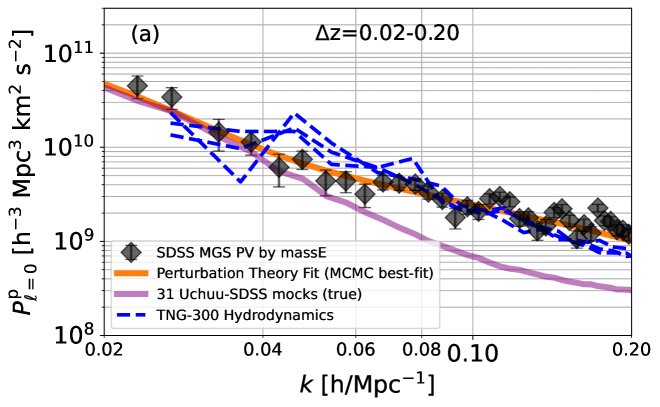
Figure 14 (a) shows the result of the momentum power spectrum of our massE-based PV sample over a redshift range of =0.02-0.2 where PV is measured with a redshift bin of =0.005. The covariance matrix is shown in Figure 15, which is based on the result from the mock. As compared to the true median of 31 Uchuu-SDSS mocks, our observed momentum power spectrum is slightly higher at low but the deviation becomes larger at 0.07 /Mpc. The difference could be the result that on small spatial scales non-linear effects affect the power spectrum, while the Uchuu-SDSS simulation is purely N-body (Ishiyama et al., 2021). In the figure, we overlay the result of TNG-300 hydrodynamics simulation that include baryons (Nelson et al., 2019). For this simulation, we use the snapshot at =0 and include all sub-halos with stellar masses larger than 1010 . The calculation of the momentum power spectrum is obtained through FFTPower implemented in nbodykit. Given a specific simulation box, we can have three lines of sight, each giving three independent measurements, as shown in the figure. The disparity between TNG and our observation above 0.07 /Mpc is now much smaller. It remains unclear what causes the difference between our observations and Uchuu-SDSS mock data. The momentum power spectrum at high is dominated by the product of the density and velocity (e.g., see Fig. 13 in Howlett (2019)). The Uchuu-SDSS mock is designed to have the same galaxy bias as the observed one, a fact we confirm by comparing the density power spectra of our observations and the Uchuu-SDSS mock. Accordingly the difference at high- should not be attributed to different galaxy biases between the two. It is probable that the N-body simulation, such as Uchuu, does not account adequately for non-linear effects as compared with TNG hydrodynamic simulation. Fortunately, the constraint on the growth rate is not particularly sensitive to the maximum wavenumber .
Figure 14(b) and (c) presents two additional momentum power spectra for two sub-redshift ranges of =0.10-0.20 and 0.02-0.10, respectively. Similar to the case of the full redshift range, the momentum power spectra within two sub-ranges exhibit a slightly elevation when compared to the Uchuu-SDSS result at low . However, they show considerably larger disparities above =0.07 /Mpc, but tend to match more or less the result of the TNG hydrodynamic simulation at high .
5.2 Robustness of the measurement
In this section, we discuss the result if varying some parameters that we use to derive the momentum power spectrum including the massE relation itself and the redshift bin .
In § 4.4, we confirm with mock data that the massE-based PV is insensitive to the accurate calibration of the massE relationship. Here we further demonstrate this with the observational data. In Figure 16(a), we overlay two momentum power spectra with the fiducial one: one is the case that the normalization of the massE relation evolves strongly with redshift as (1+)5 , and another is the one that the slope of the relationship evolves strongly with the redshift as (1+)0.4. For the , such a redshift evolution gives a value at =0.2 that deviates from the observed one by 20-. In the first case, any alteration in the value of causes all distances to shift uniformly with the same amount, thereby maintaining the offset of a distance from the Gaussian mean. As a result, the momentum power spectrum remains the same regardless of the magnitude of the shift. In the second case, the momentum power spectrum changes a little bit but well within the error bar, which still benefits from our method. For galaxies within a narrow redshift bin, their physical properties including sizes, velocity dispersions and stellar masses exhibit a narrow range. If there is a change in the slope , it only introduces a small amount of scatter in the distribution of distances. Therefore Figure 16(a) demonstrates that the momentum power spectrum with the massE-based PV is not sensitive to the accurate calibration of the massE relation. Figure 16(b) presents the momentum power spectra whose PV is measured with redshift bin sizes of =0.001 and =0.01, as compared to the fiducial one with =0.005. As shown in the figure, the three spectra are almost the same, indicating that the PV measurements is not sensitive to which can vary by a factor of 10.
6 The constraint on the growth rate
6.1 The effective survey volume
Before detailed modeling, we first roughly evaluate the statistical power of our sample in constraining a cosmological parameter, given that the signal to noise of the parameter constrained at a given is more or less proportional to the square root of the survey effective volume at that (e.g. Koda et al., 2014). Similar to the definition of the density power spectrum (Feldman et al., 1994; Tegmark, 1997), an effective volume for the momentum power spectrum can be written as
| (20) |
where and are the galaxy number density and PV variance as a function of the redshift, respectively. The above equation indicates that for high galaxy number densities /, the effective volume is just the geometrical volume and thus increases with the cube of the redshift. On the other hand, for low galaxy number densities, because roughly scales with the square of the redshift at < 0.2, the effective volume only scales linearly with the redshift.
To calculate the effective volume for our sample, we adopt the median of 31 Uchuu-SDSS mocks for . The and are shown in Figure 4 for our sample. We derived for the whole redshift range as well as two redshift sub-ranges as shown in Figure 17, along with 6dFGSv and SDSS-FP surveys. The 6dFGSv data has a spatial coverage of 17 000 deg2 and a redshift range of 0.0001 to 0.0534 (Scrimgeour et al., 2016). We use to get its velocity variance by setting =0.324 (Scrimgeour et al., 2016). The galaxy number density is almost a constant around 1.210-3 Mpc-3. We use the same as for our sample. The SDSS FP-based PV sample covers a redshift range of 0.0033 to 0.1 and an area of 7016 deg2 (Howlett et al., 2022). We use the above equation for the velocity variance with =0.23 (Howlett et al., 2022), measure from their catalog and also adopt the median of Uchuu-SDSS mocks for .
The integral quantity = gives the total number of modes on linear scales where the growth rate is sensitive to. As compared to the 6dFGSv and SDSS FP-based PV catalogs, our sample offers a factor of about 2.4 and 6.7 increase in the above quantity, respectively. As shown in the figure, even for <0.1, our effective volume is still larger than the SDSS-FP catalog, with about a factor of 1.7 larger in terms of . This is because of our larger sample even at 0.1 as presented in § 2.3. Note that, although our sample extends to =0.2, the galaxy number density above =0.1 of the SDSS MGS drops rapidly.
6.2 MCMC fitting


We use the model that is based on the distribution function and Eulerian perturbation theory as developed by Vlah et al. (2012, 2013); Okumura et al. (2014) and Saito et al. (2014). The analytic formula of the model is compiled in the appendix of Howlett (2019). Here we give the basic one:
| (21) |
where
| (22) |
The term , , and can be calculated from the linear power spectrum while containing free parameters such as the growth rate , the linear-scale bias , the non-linear bias , the non-linear velocity dispersion etc. Through these parameters the model accounts for the effect of small-scale non-linear motion on the power spectrum.
Before running the MCMC fitting, we first quantify the effect of the window function for the momentum power spectrum measurement. Due to the survey volume as well as the sample selection as a function of both spatial positions and redshift, the power spectrum suffers from the effect of the window function. We evaluate this effect using the python code pypower.CatalogSmoothWindow333https://github.com/cosmodesi/pypower with following steps: (1) a random elliptical catalog: we start with a random catalog available for the SDSS LSS sample444http://sdss.physics.nyu.edu/vagc/lss.html, http://sdss.physics.nyu.edu/lss/dr72/ (Blanton et al., 2005). We first follow the observed fraction of ellipticals in the LSS sample to randomly pick objects from the above catalog to define the random elliptical catalog. By fitting the observed redshift distribution of the MGS-elliptical sample with multiple Gaussian profiles, we assign a random redshift to those in the random elliptical catalog. After that, we remain those in the North Cap region and limit the redshift range to 0.02-0.2. (2) the window function: based on the above random catalog, we then use pypower.CatalogSmoothWindow to derive multipoles of the window function up to =9 with the wide angle up to the order of =1. The result in the configuration space is shown in Figure 18(a) for =0.02-0.20. (3) the theory power spectrum: we then use Equation 21 to produce theoretical momentum power spectrum at =0, 2 & 4 with from 0.001 to 10 with a resolution of 0.005. (4) the power spectrum with window function and wide angle: we then convolve the above theoretical momentum power spectrum with the window function and wide-angle, and show its ratio to the pure theoretical spectrum in Figure 18(b). It is found that the effect of the window function and wide-angle is small but a difference of a few to ten percent is seen for values between 0.02 and 0.1 /Mpc. We thus carry out the MCMC fitting by incorporating correction factors into the theoretical power spectrum. The correction factors for two redshift sub-ranges of =0.02-0.10 and =0.10-0.20 are also produced following the same procedure, and their differences from the above one are small.
As discussed in Qin et al. (2019), the distribution of the momentum power spectrum at given is not always normal as shown in Fig. 19(a), and it is thus suggested to first Box-Cox transform (Box & Cox, 1964) the momentum power spectrum to for which the MCMC fitting is carried out:
| (23) |
Here, because of large errors in some P() is negative so that we add a which is set to be the minimum negative value of the distribution. The code scipy.stats.boxcox is used to find the best for each transformation.
We set the background cosmological parameter to the Planck 2018 result with (=0)=0.811 (Planck Collaboration et al., 2020), based on which the linear power spectrum at =0 is calculated as an input of the theoretical power spectrum through nbodykit using the CLASS transfer function. In this case, if we multiply the derived with (=0), it gives at . Following Qin et al. (2019), we set the following four free parameters: , , and . The MCMC fitting has been carried out through Python code emcee (Foreman-Mackey et al., 2013). Priors of four parameters are listed in Table 2.
We set /Mpc and conduct the MCMC fitting for values of 0.15, 0.20 and 0.25 /Mpc, respectively, for galaxies within z=0.02-0.2. The corner plots of three fitting results are shown in Figure 20. The growth rate remains unaffected by the non-linear parameters and . While there are some correlations between and at a given , the best-fit values of exhibit no sensitivity to . This is consistent with the expected advantage of the momentum power spectrum that is affected little by the bias and non-linear effects. Figure 22 offers a further comparison in between observations and Uchuu-SDSS mocks, revealing that our observations and the mock data conform to the predictions of General Relativity (GR) and display no trends with respect to . The errors from observation are slightly larger than those from mocks. This is reasonable because the median momentum power spectrum of mocks at each almost precisely lies on the theoretical prediction. As shown in Figure 23, the best fit is slightly below the median of data points, which is caused by the fact that the covariance matrix contains significant non-diagonal parts. This is also the reason that the best-fitted of mocks are not exactly but slightly smaller than the GR’s prediction.
As shown in Figure 20 and Figure 21, there are noticeable discrepancies in the best-fit between observations and mocks. This discrepancy is indicative of a disparity in the momentum power spectrum at high regime between the two as shown in Figure 14. While both observations and mocks have a similar galaxy bias ( 1.5) as seen by their density power spectrum, the difference in the above result is likely due to the velocity field on small scales. As stated above, the comparison between Uchuu-SDSS and TNG indicates that Uchuu-SDSS as a N-body simulation may not fully account for non-linear effects. In addition, the observations exhibit higher values than TNG above = 0.1 /Mpc by about 20-30%. There may be two reasons for this: one is that there is some random zero-point offsets in velocity similar to those seen in mock simulations (see Figure 9), which adds a constant to the shot noise (Howlett, 2019). This addition predominantly affects the high- regime but becomes negligible at low-; another is that since the mocks underestimate the power at high-, the corresponding error at high- is also underestimated. Nevertheless, these factors should not affect our conclusion regarding , as it primarily relies on the low regime.
We also carry out fit to the momentum power spectra of two sub-redshift ranges of =0.02-0.1 and 0.1-0.2, which gives of 0.416 and 0.526, respectively, for =0.20 /Mpc. As shown in Figure 23, they are consistent with the result of the entire redshift range, which yields a value of 0.459, well within the 1- confidence interval. The inverse variance of for the whole redshift range is almost the same as the sum of those of two redshift sub-ranges too. These results offer additional evidence for the robustness of our results.
Table 2 lists /d.o.f. values for three redshift ranges, which are between 2 and 3. We suspect that this is due to the fact that the mock data under-estimate the momentum power spectra and associated errors at high values as stated in § 5.1. To test this for =0.02-0.2, we increase the error by a factor of 1.5 for above 0.1 /Mpc and corresponding non-diagonal parts in the covariance matrix. By carrying out the MCMC fitting again, it is found that the best-fit remains unchanged but now /d.o.f. is 36/32. This further demonstrates that the growth rate measured from momentum power spectrum is insensitive to momentum power spectra on small scales.
6.3 Comparisons with other studies
Qin et al. (2019) adopted the same theoretical model with the same set of free parameters for the 6dFGSv and 2MTF PV data. They obtained =0.404 with the combined density power spectrum and momentum power spectrum of two data-sets together.This constraint is similar to that by Turner et al. (2023) using the combined velocity and density data of the 6dFGSv survey. If adopting the momentum power spectrum of the 6dFGSv survey alone, Qin et al. (2019) estimated 68% confidence range to be 0.226 (see their Table 2). Our measurement from = offers a factor of 1.7 higher accuracy. This improvement in accuracy is somewhat less than that expected by the square root of the increase in the effective volume (6.7), but are consistent within 30%. This is reasonable given different mocks or fitting techniques (Eisenstein et al., 2005). Lai et al. (2023) measured the growth rate using the maximum-likelihood fields method through both density and PV data of the SDSS-FP survey (Howlett et al., 2022). The derived growth rate is 0.405(stat)0.009 (sys), whose confidence range is consistent with our low- one (0.416 for =0.02-0.1). They did not report the result when only using PV data. However, as mentioned earlier, although both our catalog and the SDSS-FP catalog are based on the same parent sample, our massE-based PV catalog includes 2.5 more objects than the SDSS-FP catalog at < 0.1. This could account for our PV-only result exhibiting a similar level of error as theirs of combined PV and density data. Saulder et al. (2023) have provided the predicted number density and PV error for the DESI survey, from which they estimated a 68% confidence range for , which is 0.126 and 0.092 for values of 0.1 /Mpc and 0.2 /Mpc, respectively. We measure their effective volume and find that their number of -modes between 0.02 and 0.07 /Mpc is 1.7 times more than our entire redshift range. This corresponds to a 1.3-fold enhancement in their precision, consistent with our constraint of at a value of 0.459 at =0.2 /Mpc.
Howlett et al. (2015) measured the redshift space distortion of the SDSS MGS sample through two-point correlation function, resulting in a derived of 0.49. Our massE-based PV measurement of the same sample thus offers a factor of 2.1 improvement in the error of . In Figure 24, we overlay our measurement on most recent collection of that has been measured with redshift space distortion (Alam et al., 2021).
| par. name | priors | =0.02-0.1 | =0.1-0.2 | =0.02-0.2 |
|---|---|---|---|---|
| (, ) | (0.02, 0.20) | (0.02, 0.20) | (0.02, 0.20) | |
| 0.0666 | 0.1363 | 0.0959 | ||
| (GR) | 0.4448 | 0.4574 | 0.4505 | |
| U(0, 5) | 0.416 | 0.526 | 0.459 | |
| U(0, 10) | 2.36 | 2.68 | 2.33 | |
| U(0,50) | 16.32 | 15.17 | 16.68 | |
| [/Mpc] | U(0,inf) | 1.28 | 1.20 | 1.16 |
| /d.o.f. | 75.5/31 | 91.1/32 | 65.5/32 |
U stands for a uniform distribution. The error of the best fit is given for the 68% confidence range.


6.4 Fisher-matrix forecast for the massE-based PV
Our work has demonstrated that the massE can serve as a new cosmic ruler with only two nuisance parameters, allowing for the probing of the PV beyond the current redshift limit of 0.1. For future perspective, we envision that there is no apparent limit for the PV measurement with the massE to higher redshift, as it is insensitive to the accurate calibration of the massE relation itself. In addition, because of term in Equation 10 that is used to convert the distance measurement to PV, the PV variance scales with the redshift slower than by a few times, especially above =0.2, as shown in Figure 25(a). As a result, although measuring the momentum power spectrum still requires a high galaxy number density above =0.2, it has a potential to provide strong constraints on the growth rate in the late universe where dark energy dominates. To illustrate this quantitatively, we use the Fisher-matrix forecast code555https://github.com/CullanHowlett/PV_fisher (Howlett et al., 2017; da Cunha et al., 2017) with a survey area of 14 k square degree, a distance error of =20%, a galaxy number density of 810-3 /Mpc3 and Equation 10 for the PV error. As shown in Figure 25(a), PV-only data yields stronger constraints compared to the RSD only for this specific data-set where is set to be 0.2 /Mpc. On the other hand, the momentum power spectrum mainly relies on linear scales to extract cosmological information, complementing the RSD. The combination of these two offers significant improvement in the growth rate, potentially exceeding the DESI’s constraints by a factor of 1.7 to 4.7 in terms of errors.
7 Conclusions
In this study we utilize the massE relation of galaxies as a new cosmic ruler to estimate the PV of SDSS MGS elliptical galaxies from =0.02 out to =0.2, and measure their momentum power spectrum. The main conclusions are as followings:
(1) PV is measured for a galaxy based on the offset of its massE-based distance from the Gaussian mean of the distance distribution in a narrow redshift bin.
(2) The final PV catalog consists of 229,890 objects, which is almost seven times larger than the previously largest catalog. The redshift coverage is well beyond the limit of around 0.1 in literature studies using other distance rulers such as Tully-Fisher and FP.
(3) By mimicking the PV measurements with our method in Uchuu-SDSS mock galaxies, we show that both the PV of individual galaxies and the momentum power spectra can be recovered well, and both are insensitive to accurate calibration of the massE relation itself.
(4) We derive the momentum power spectrum based on the massE-based PV catalog over spatial scales from 0.02 to 0.2 h/Mpc. The spectrum shows little dependence on the massE relation, including its slope and intercept. The derived spectra for two sub-redshift ranges of 0.02-0.10 and 0.10-0.20 are consistent with the one over the whole redshift range. The spectrum is also insensitive to the size of the redshift bin in which PV is measured. These demonstrate the robust of the massE-based PV measurement.
(5) By fitting perturbation theory model to the derived momentum power spectrum with four free parameters, we find the best-fit to be 0.459 at =0.0959. Its error is 2.1 times smaller than the value based on the redshift space distortion of the SDSS MGS.
(6) The massE-based PV is insensitive to accurate calibration of the massE relation itself. This combined with a slow increase in the PV errors with redshift beyond =0.2, makes the massE-based PV a potentially competitive new method to offer high-precision constraints on the growth rate, in addition to the RSD.
Acknowledgements
We thank the anonymous referee for detailed and constructive comments that improved the manuscript significantly. Y.S. acknowledges the support from the National Key R&D Program of China No. 2022YFF0503401, the National Natural Science Foundation of China (NSFC grants 11825302, 12141301, 12121003, 12333002), and the New Cornerstone Science Foundation through the XPLORER PRIZE.
Funding for the SDSS and SDSS-II has been provided by the Alfred P. Sloan Foundation, the Participating Institutions, the National Science Foundation, the U.S. Department of Energy, the National Aeronautics and Space Administration, the Japanese Monbukagakusho, the Max Planck Society, and the Higher Education Funding Council for England. The SDSS Web Site is http://www.sdss.org/. The SDSS is managed by the Astrophysical Research Consortium for the Participating Institutions. The Participating Institutions are the American Museum of Natural History, Astrophysical Institute Potsdam, University of Basel, University of Cambridge, Case Western Reserve University, University of Chicago, Drexel University, Fermilab, the Institute for Advanced Study, the Japan Participation Group, Johns Hopkins University, the Joint Institute for Nuclear Astrophysics, the Kavli Institute for Particle Astrophysics and Cosmology, the Korean Scientist Group, the Chinese Academy of Sciences (LAMOST), Los Alamos National Laboratory, the Max-Planck-Institute for Astronomy (MPIA), the Max-Planck-Institute for Astrophysics (MPA), New Mexico State University, Ohio State University, University of Pittsburgh, University of Portsmouth, Princeton University, the United States Naval Observatory, and the University of Washington.
Data Availability
The data produced here are available upon reasonable request.
References
- Adams & Blake (2017) Adams C., Blake C., 2017, MNRAS, 471, 839
- Adams & Blake (2020) Adams C., Blake C., 2020, MNRAS, 494, 3275
- Alam et al. (2017) Alam S., et al., 2017, MNRAS, 470, 2617
- Alam et al. (2021) Alam S., et al., 2021, Phys. Rev. D, 103, 083533
- Beutler et al. (2012) Beutler F., et al., 2012, MNRAS, 423, 3430
- Blake et al. (2012) Blake C., et al., 2012, MNRAS, 425, 405
- Blanton et al. (2005) Blanton M. R., et al., 2005, AJ, 129, 2562
- Box & Cox (1964) Box G. E. P., Cox J. R., 1964, J. R. Stat. Soc., 26, 211
- Brinchmann et al. (2004) Brinchmann J., Charlot S., White S. D. M., Tremonti C., Kauffmann G., Heckman T., Brinkmann J., 2004, MNRAS, 351, 1151
- Castorina & White (2018) Castorina E., White M., 2018, MNRAS, 476, 4403
- DESI Collaboration et al. (2016) DESI Collaboration et al., 2016, arXiv e-prints, p. arXiv:1611.00036
- Dong-Páez et al. (2022) Dong-Páez C. A., et al., 2022, arXiv e-prints, p. arXiv:2208.00540
- Dressler et al. (1987) Dressler A., Lynden-Bell D., Burstein D., Davies R. L., Faber S. M., Terlevich R., Wegner G., 1987, ApJ, 313, 42
- Eisenstein et al. (2005) Eisenstein D. J., et al., 2005, ApJ, 633, 560
- Feldman et al. (1994) Feldman H. A., Kaiser N., Peacock J. A., 1994, ApJ, 426, 23
- Fixsen et al. (1996) Fixsen D. J., Cheng E. S., Gales J. M., Mather J. C., Shafer R. A., Wright E. L., 1996, ApJ, 473, 576
- Foreman-Mackey et al. (2013) Foreman-Mackey D., Hogg D. W., Lang D., Goodman J., 2013, PASP, 125, 306
- Gil-Marín et al. (2020) Gil-Marín H., et al., 2020, MNRAS, 498, 2492
- Hand et al. (2017) Hand N., Li Y., Slepian Z., Seljak U., 2017, J. Cosmology Astropart. Phys., 2017, 002
- Hand et al. (2018) Hand N., Feng Y., Beutler F., Li Y., Modi C., Seljak U., Slepian Z., 2018, AJ, 156, 160
- Howlett (2019) Howlett C., 2019, MNRAS, 487, 5209
- Howlett et al. (2015) Howlett C., Ross A. J., Samushia L., Percival W. J., Manera M., 2015, MNRAS, 449, 848
- Howlett et al. (2017) Howlett C., Staveley-Smith L., Blake C., 2017, MNRAS, 464, 2517
- Howlett et al. (2022) Howlett C., Said K., Lucey J. R., Colless M., Qin F., Lai Y., Tully R. B., Davis T. M., 2022, arXiv e-prints, p. arXiv:2201.03112
- Ishiyama et al. (2021) Ishiyama T., et al., 2021, MNRAS, 506, 4210
- Johnson et al. (2014) Johnson A., et al., 2014, MNRAS, 444, 3926
- Kaiser (1987) Kaiser N., 1987, MNRAS, 227, 1
- Kauffmann et al. (2003) Kauffmann G., et al., 2003, MNRAS, 341, 33
- Koda et al. (2014) Koda J., et al., 2014, MNRAS, 445, 4267
- Lahav et al. (1991) Lahav O., Lilje P. B., Primack J. R., Rees M. J., 1991, MNRAS, 251, 128
- Lai et al. (2023) Lai Y., Howlett C., Davis T. M., 2023, MNRAS, 518, 1840
- Linder & Cahn (2007) Linder E. V., Cahn R. N., 2007, Astroparticle Physics, 28, 481
- Magoulas et al. (2012) Magoulas C., et al., 2012, MNRAS, 427, 245
- Masters et al. (2008) Masters K. L., Springob C. M., Huchra J. P., 2008, AJ, 135, 1738
- Nelson et al. (2019) Nelson D., et al., 2019, Computational Astrophysics and Cosmology, 6, 2
- Neveux et al. (2020) Neveux R., et al., 2020, MNRAS, 499, 210
- Okumura et al. (2014) Okumura T., Seljak U., Vlah Z., Desjacques V., 2014, J. Cosmology Astropart. Phys., 2014, 003
- Okumura et al. (2016) Okumura T., et al., 2016, PASJ, 68, 38
- Peebles (1980) Peebles P. J. E., 1980, The large-scale structure of the universe
- Pezzotta et al. (2017) Pezzotta A., et al., 2017, A&A, 604, A33
- Planck Collaboration et al. (2020) Planck Collaboration et al., 2020, A&A, 641, A6
- Qin et al. (2019) Qin F., Howlett C., Staveley-Smith L., 2019, MNRAS, 487, 5235
- Riess et al. (1998) Riess A. G., et al., 1998, AJ, 116, 1009
- Saito et al. (2014) Saito S., Baldauf T., Vlah Z., Seljak U., Okumura T., McDonald P., 2014, Phys. Rev. D, 90, 123522
- Saulder et al. (2023) Saulder C., et al., 2023, arXiv e-prints, p. arXiv:2302.13760
- Scrimgeour et al. (2016) Scrimgeour M. I., et al., 2016, MNRAS, 455, 386
- Shi et al. (2021) Shi Y., Yu X., Mao S., Gu Q., Xia X., Chen Y., 2021, MNRAS, 507, 2423
- Shi et al. (2022) Shi Y., Chen Y., Mao S., Gu Q., Wang T., Xia X., Zhang. Z.-Y., 2022, MNRAS, 516, 1662
- Springob et al. (2014) Springob C. M., et al., 2014, MNRAS, 445, 2677
- Tegmark (1997) Tegmark M., 1997, Phys. Rev. Lett., 79, 3806
- Tonry & Schneider (1988) Tonry J., Schneider D. P., 1988, AJ, 96, 807
- Tonry et al. (2001) Tonry J. L., Dressler A., Blakeslee J. P., Ajhar E. A., Fletcher A. B., Luppino G. A., Metzger M. R., Moore C. B., 2001, ApJ, 546, 681
- Tully & Fisher (1977) Tully R. B., Fisher J. R., 1977, A&A, 500, 105
- Tully et al. (2022) Tully R. B., et al., 2022, arXiv e-prints, p. arXiv:2209.11238
- Turner et al. (2023) Turner R. J., Blake C., Ruggeri R., 2023, MNRAS, 518, 2436
- Vlah et al. (2012) Vlah Z., Seljak U., McDonald P., Okumura T., Baldauf T., 2012, J. Cosmology Astropart. Phys., 2012, 009
- Vlah et al. (2013) Vlah Z., Seljak U., Okumura T., Desjacques V., 2013, J. Cosmology Astropart. Phys., 2013, 053
- Wang et al. (2021) Wang Y., Peery S., Feldman H. A., Watkins R., 2021, ApJ, 918, 49
- Yamamoto et al. (2006) Yamamoto K., Nakamichi M., Kamino A., Bassett B. A., Nishioka H., 2006, PASJ, 58, 93
- da Cunha et al. (2017) da Cunha E., et al., 2017, Publ. Astron. Soc. Australia, 34, e047
- de Mattia et al. (2021) de Mattia A., et al., 2021, MNRAS, 501, 5616