Precision Neutron Decay Matrix Elements (PNDME) Collaboration
Moments of nucleon isovector structure functions in -flavor QCD
Abstract
We present results on the isovector momentum fraction, , helicity moment, , and the transversity moment, , of the nucleon obtained using nine ensembles of gauge configurations generated by the MILC Collaboration using -flavors of dynamical highly improved staggered quarks (HISQ). The correlation functions are calculated using the Wilson-Clover action and the renormalization of the three operators is carried out nonperturbatively on the lattice in the scheme. The data have been collected at lattice spacings and 0.06 fm and and 135 MeV, which are used to obtain the physical values using a simultaneous chiral-continuum-finite-volume fit. The final results, in the scheme at 2 GeV, are , and , where the first error is the overall analysis uncertainty and the second is an additional systematic uncertainty due to possible residual excited-state contributions. These results are consistent with other recent lattice calculations and phenomenological global fit values.
pacs:
11.15.Ha, 12.38.GcI Introduction
| Ensemble | |||||||||
| ID | [fm] | [MeV] | |||||||
The elucidation of the hadron structure in terms of quarks and gluons is evolving from determining the charges and form factors of nucleons to including more complex quantities such as parton distribution functions (PDFs) Brock et al. (1995), transverse momentum dependent PDFs (TMDs) Yoon et al. (2017a), and generalized parton distributions (GPDs) Diehl (2003) as experiments become more precise Accardi et al. (2016a); Boer et al. (2011). These distributions are not measured directly in experiments, and phenomenological analyses including different theoretical inputs are needed to extract them from experimental data. Input from lattice QCD is beginning to play an increasingly larger role in such analyses Lin et al. (2018). In cases where both lattice results and phenomenological analyses of experimental data (global fits) exist, one can compare them to validate the control over systematics in the lattice calculations, and, on the other hand, provide a check on the phenomenological process used to extract these observables from experimental data. In other cases, lattice results are predictions. The list of quantities for which good agreement between lattice calculations and experimental results, and their precision, has grown very significantly as discussed in the recent Flavor Lattice Averaging Group (FLAG) 2019 report Aoki et al. (2020). While steady progress has been made in developing the framework for calculating distribution functions using lattice QCD Cichy and Constantinou (2019); Karthik (2019), even calculations of their moments have had large statistical and/or systematic uncertainties prior to 2018. This was the case even for the best studied quantity, the isovector momentum fraction Lin et al. (2018). In this work, we show that the lattice data for the momentum fraction, helicity and transversity moments are now of quality comparable to that for nucleon charges (zeroth moments). Together with much more precise data from the planned electron-ion collider Accardi et al. (2016a) and the Large Hadron Collider, which will significantly improve the phenomenological global fits, we anticipate steady progress toward a detailed description of the hadron structure.
In this paper we present results on the three moments from high statistics calculations done on nine ensembles generated using 2+1+1-flavors of highly improved staggered quarks (HISQ) Follana et al. (2007) by the MILC Collaboration Bazavov et al. (2013). The data at four values of lattice spacings , three values of the pion mass, , including two ensembles at the physical pion mass, and on a range of large physical volumes, characterized by , allow us to carry out a simultaneous fit in these three variables to address the associated systematics uncertainties. We also investigate the dependence of the results on the spectra of possible excited states included in the fits to remove excited-state contamination (ESC), and assign a second error to account for the associated systematic uncertainty. Our final results are , and in the scheme at 2 GeV. On comparing these with other lattice and phenomenological global fit results in Sec. VI, we find a consistent picture emerging.
The paper is organized as follows: In Sec. II, we briefly summarize the lattice parameters and methodology. The definitions of moments and operators investigated are given in Sec. III. The two- and three-point functions calculated, and their connection to the moments, are specified in Sec. IV, and the analysis of excited state contributions to extract ground state matrix elements is presented in Sec. V. Results for the moments after the chiral-continuum-finite-volume (CCFV) extrapolation are given in Sec. VI, and compared with other lattice calculations and global fits. We end with conclusions in Sec. VII. The data and fits used to remove excited-state contamination are shown in Appendix A and the results for renormalization factors, , for the three operators in Appendix B.
II Lattice Methodology
The parameters of the nine HISQ ensembles are summarized in Table 1. They cover a range of lattice spacings ( fm), pion masses () MeV and lattice sizes (). Most of the details of the lattice methodology, the strategies for the calculations and the analyses are already given in Refs. Bhattacharya et al. (2015, 2016); Gupta et al. (2018). We construct the correlation functions needed to calculate the matrix elements using Wilson-clover fermions on these HISQ ensembles. This mixed-action, clover-on-HISQ, formulation is nonunitary and can suffer from the problem of exceptional configurations at small, but a priori unknown, quark masses. We have not found evidence for such exceptional configurations on any of the nine ensembles analyzed in this work.
For the parameters used in the construction of the - and -point functions with Wilson-clover fermion see Table II of Ref. Gupta et al. (2018). The Sheikholeslami-Wohlert coefficient Sheikholeslami and Wohlert (1985) used in the clover action is fixed to its tree-level value with tadpole improvement, , where is the fourth root of the plaquette expectation value calculated on the hypercubic (HYP) smeared Hasenfratz and Knechtli (2001) HISQ lattices.
The masses of light clover quarks were tuned so that the clover-on-HISQ pion masses, , match the HISQ-on-HISQ Goldstone ones, . values are given in Table 1. values are available in Ref. Gupta et al. (2018). All fits in to study the chiral behavior are made using the clover-on-HISQ since the correlation functions, and thus the chiral behavior of the moments, have a greater sensitivity to it. Henceforth, for brevity, we drop the superscript and denote the clover-on-HISQ pion mass as . The number of high precision (HP) and low precision (LP) measurements made on each configuration in the truncated solver bias corrected method Bali et al. (2010); Blum et al. (2013) for cost-effective increase in statistics are specified in Table 1.
III Moments and Matrix elements
In this work, we calculate the first moments of spin independent (or unpolarized), , helicity (or polarized), , and transversity, distributions, defined as
| (1) | |||||
| (2) | |||||
| (3) |
where corresponds to quarks with helicity aligned (antialigned) with that of a longitudinally polarized target, and corresponds to quarks with spin aligned (antialigned) with that of a transversely polarized target.
These moments, at leading twist, can be extracted from the hadron matrix elements of one-derivative vector, axial-vector and tensor operators at zero momentum transfer. The unpolarized and polarized moments and of the nucleon are also obtained from phenomenological global fits while a computation of the nucleon transversity using lattice QCD is still a prediction due to the lack of sufficient experimental data Lin et al. (2018).
We are interested in extracting the forward nucleon matrix elements , with the nucleon initial and final 3-momenta, , taken to be zero in this work. The complete set of one-derivative vector, axial-vector, and tensor operators is the following:
| (12) | |||||
| (21) | |||||
| (30) |
where is the isodoublet of light quarks and . The derivative consists of four terms:
| (31) | |||||
Lorentz indices within in Eq. (30) are symmetrized and within are antisymmetrized. It is also implicit that, where relevant, the traceless part of the above operators is taken. Their renormalization is carried out nonperturbatively in the regularization independent RI′-MOM scheme as discussed in Appendix B. A more detailed discussion of these twist-2 operators and their renormalization can be found in Refs. Gockeler et al. (1996); Harris et al. (2019).
In this work, we consider only isovector quantities. These are obtained from Eq. (30) by choosing for the Pauli matrix. The decomposition of the matrix elements of these operators in terms of the generalized form factors at zero momentum transfer is as follows:
| (32) | ||||
| (33) | ||||
| (34) |
The relation between the momentum fraction, the helicity moment, and the transversity moment, and the generalized form factors is , and respectively.
IV Correlation functions and Moments
We use the following interpolating operator to create/annihilate the nucleon state
| (35) |
where are color indices, and is the charge conjugation matrix. The nonrelativistic projection is inserted to improve the signal, with the plus and minus signs applied to the forward and backward propagation in Euclidean time, respectively Gockeler et al. (1996). At zero momentum, this operator couples only to the spin state. The zero momentum 2-point and 3-point nucleon correlation functions are defined as
| (36) | ||||
| (37) |
where and are spin indices. The source is placed at time slice 0, the sink is at and the one-derivative operators, defined in Sec. III, are inserted at time slice . Data have been accumulated for the values of specified in Table 1, and in each case for all intermediate times .
To isolate the various operators, projected - and -point functions are constructed as
| (38) | |||||
| (39) |
The projector in the nucleon correlator gives the positive parity contribution for the nucleon propagating in the forward direction. For the connected -point contributions is used. With these spin projections, the explicit operators used to calculate the forward matrix elements are:
| (56) | |||||
| (65) | |||||
| (74) |
Our goal is to obtain the matrix elements, (), of these operators within the ground state of the nucleon. These are related to the moments as follows:
| (75) | |||||
| (76) | |||||
| (77) |
where is the nucleon mass. The three moments are dimensionless, and their extraction on a given ensemble does not require knowing the value of the lattice scale . It enters only when performing the chiral-continuum extrapolation to the physical point as discussed in Sec. VI.
| Ensemble | Observable | /dof | /dof | ||||||
| Ensemble | Fit-type | /dof | |||||||
| – | – | – | – | ||||||
| Ensemble | Fit-type | /dof | |||||||
| Ensemble | Fit-type | /dof | |||||||
| – | – | – | – | ||||||
V Controlling excited state contamination
To calculate the matrix elements of the operators defined in Sec. III between ground-state nucleons, contributions of all possible excited states need to be removed. The lattice nucleon interpolating operator given in Eq. (35), however, couples to the nucleon, all its excitations and multiparticle states with the same quantum numbers. Previous lattice calculations have shown that the ESC can be large Bhattacharya et al. (2014); Bali et al. (2014, 2012). In our earlier works Bhattacharya et al. (2015, 2016); Gupta et al. (2018); Yoon et al. (2016), we have shown that this can be controlled to within a few percent. We use the same strategy here. In particular, we use HYP smearing of the gauge links before calculating Wilson-clover quark propagators with optimized Gaussian smeared sources using the multigrid algorithm Babich et al. (2010); Clark et al. (2010). Correlation functions constructed from these smeared source propagators have smaller excited state contamination Yoon et al. (2016). To extract the ground state matrix elements from these, we fit the three-point data at several -values (listed in Table 1) simultaneously using the spectral decomposition given in Eq. (79).
Fits to the zero-momentum two-point functions, , were carried out keeping up to four states in the spectral decomposition:
| (78) |
Fits are made over a range to extract and , the masses and the amplitudes for the creation/annihilation of these states by the interpolating operator . In fits with more than two states, estimates of the amplitudes and masses for were sensitive to the choice of the starting time slice . We used the largest time interval allowed by statistics, i.e., by the stability of the covariance matrix. We perform two types of 4-state fits. In the fit denoted , we use the empirical Bayesian technique described in Ref. Yoon et al. (2017b) to stabilize the three excited-state parameters. In the second fit, denoted , we use as prior for either the noninteracting energy of or the state, which are both lower than the obtained from the fit, and roughly equal for the nine ensembles. The lower energy state has been shown to contribute in the axial channel Jang et al. (2020), whereas for the vector channel the state is expected to be the relevant one. We find that these two fits to the two-point function cannot be distinguished on the basis of the dof, in fact, the full range of between the two estimates from and are viable first-excited-state masses on the basis of dof alone. The same is true of the values for . We therefore, investigate the dependence of the results for moments on the exited-state spectra by doing the full analysis with multiple strategies as discussed below. The ground-state nucleon mass obtained from the various fits is denoted by the common symbol and the mass gaps by .
The analysis of the zero-momentum three-point functions, , is performed retaining up to three states in the spectral decomposition:
| (79) |
The operators, , are defined in Eqs. (56), (65) and (74). By fixing the momentum at the sink to zero and inserting the operator at zero momentum transfer we get the forward matrix element. The practical challenge discussed above is determining the relevant and to use, and, failing that, to investigate the sensitivity of to possible values of and and including that variation as a systematic uncertainty.
| Fit-type | Observable | /dof | ||||
|---|---|---|---|---|---|---|
| CC | ||||||
| CC | ||||||
| CC | ||||||
| CCFV | ||||||
| CCFV | ||||||
| CCFV |
For all the strategies used to determine and , we extract the desired ground state matrix element by fitting the three-point correlators for a subset of values of and simultaneously. This subset is chosen to reduce ESC—we select the largest values of and discard number of points next to the source and sink for each . These values of and of are given in Table 2.
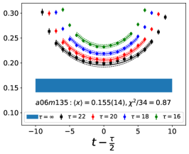
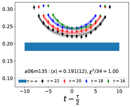
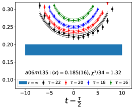
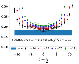
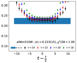
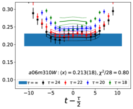
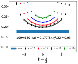
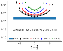
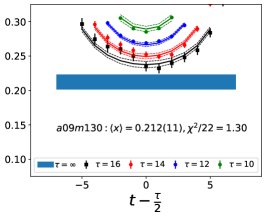
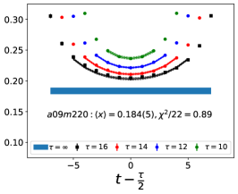
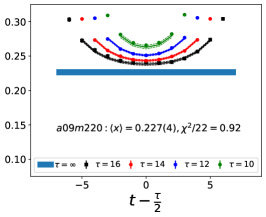
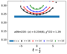
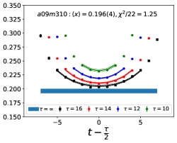
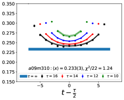
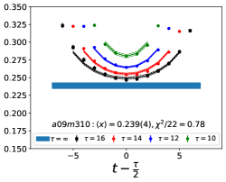
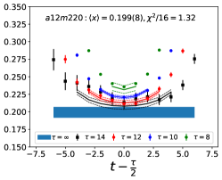
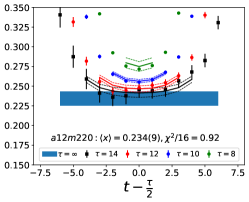
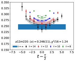
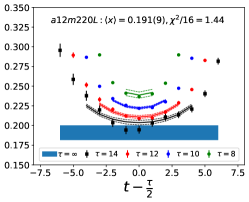
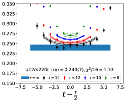
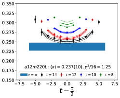
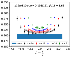
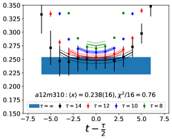
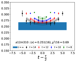
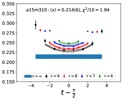
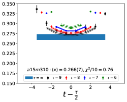
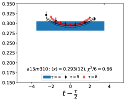
The data for the ratio are shown in Figs. 5 and 6 in the Appendix A for all nine ensembles. The signal in the three-point correlators decreases somewhat from momentum fraction to helicity moment to transversity moment. Nevertheless, we are able to make state (3-state with ) fits in all cases. The spectral decomposition predicts that the data for all three quantities is symmetric about , however, on some of the ensembles, and for some of the larger values of , the data show some asymmetry, which is indicative of the size of statistical fluctuations that are present.
The fits to and are carried out within a single-elimination jackknife process, which is used to get both the central values and the errors.
We have investigated five fit types, , , , and , based on the spectral decomposition to understand and control ESC. The labels denote an -state fit to the two-point function and an -state fit to the three-point function. In the -fit to the three-point function, is left as a free parameter, while a -fit is a 3-state fit with . The results from the five strategies for the momentum fraction, , in Table 3, for the helicity moment, , in Table 4, and for the transversity moment, , in Table 5 illustrate the observed behavior for the ensemble, which has the highest statistics, and the physical mass ensemble at the smallest value of .
For all three observables, the five results in Tables 3, 4, and 5 for the ground state matrix element, , are consistent within on the ensemble. On the ensemble, the difference in between and analyses becomes roughly a factor of 2, and from the fit is larger than even the value, i.e., the fit does not prefer the small given by . On the other hand, the from a two-state fit is expected to be larger since it is an effective combination of the mass gaps of the full tower of excited states. Due to a small , fits with the spectrum from fail on , whereas, on both ensembles, the and fits give results consistent within . The estimates from these two fit-types are given in Table 2. To summarize, our overall strategy is to keep as many excited states as possible without overparameterization of the fits. We, therefore, choose, for the central values, the results, and to take into account the spread due to the fit-type, we add a second, systematic, uncertainty to the final results in Table 7. This is taken to be the difference between the results obtained by doing the full analysis with the and strategies.
The renormalization of the matrix elements is carried out using estimates of , and calculated on the lattice in the scheme and then converted to the scheme at 2 GeV as described in Appendix B. The final values of , and used in the analysis are given in Table 9.
| Observable | Best estimate | ||
|---|---|---|---|
| 0.173(14) | 0.180(14) | 0.173(14)(07) | |
| 0.213(15) | 0.235(15) | 0.213(15)(22) | |
| 0.208(19) | 0.236(18) | 0.208(19)(24) |
VI Chiral, continuum and infinite volume extrapolation
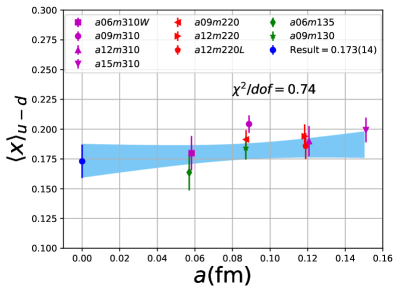
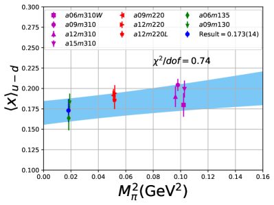
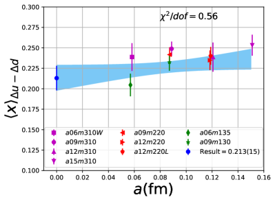
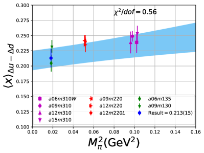
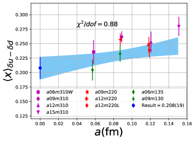
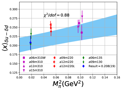
To obtain the final, physical results at MeV, and , we make a simultaneous CCFV fit keeping only the leading correction term in each variable:
| (80) |
Note that, since the operators are not improved and we used the Clover-on-HISQ formulation, we take the discretization errors to start with a term linear in . The fits to the data from the nine ensembles are shown in Figs. 1, 2 and 3. The fit parameters are summarized in Table 6.
The results of the CCFV fits show that the finite volume correction term, , is not constrained. We therefore, also present results from a CC fit, i.e., with in Eq. (80). Results for from the two fit ansatz overlap and there is a small positive slope in both and for all three quantities. The data for both and , given in Table 2, are very similar, but with a systematic shift of about 0.01–0.02 in all three cases. This difference arises because for is larger (except in ) and because the convergence with respect to is from above as shown in Figs. 5 and 6, i.e., a larger implies a smaller extrapolation and a larger value.
For our final results we quote the CC fit values as the coefficient of the finite-volume corrections in the CCFV fits is undetermined. The CC results with the two strategies, and , are summarized in Table 7. For our best estimates, we take the results and add a second, systematic, error that is the difference between these two strategies and represents the uncertainty in controlling the excited-state contamination.
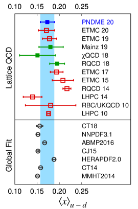
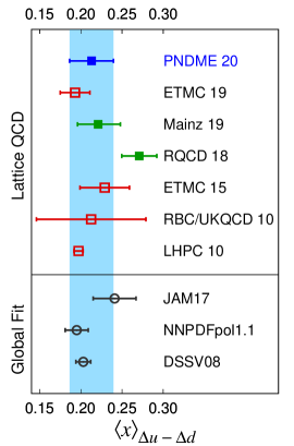
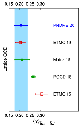
A comparison of these results with other lattice QCD calculations on ensembles with dynamical fermions is presented in the top half of Table 8 and shown in Fig. 4. Our results agree with those from the Mainz group Harris et al. (2019) that have also been obtained using data on a comparable number of ensembles, but all with MeV, which are used to perform a chiral and continuum extrapolation. The one difference is the slope of the chiral correction. For our clover-on-HISQ formulation, we find a small positive value while the Mainz data show a small negative value Harris et al. (2019). Our results are also consistent within 1 with the ETMC 20 Alexandrou et al. (2020a) and ETMC 19 Alexandrou et al. (2020b) values that are from a single physical mass ensemble. The central value from QCD Yang et al. (2018), using partially quenched analysis, is smaller but consistent within . Results for the momentum fraction and the helicity moment from RQCD 18 Bali et al. (2019) are taken from their Set A with the difference between Set A and B values quoted as a second systematic uncertainty. Their result for the transversity moment is from a single MeV ensemble. These values are larger, especially for the helicity and transversity moment. Other earlier lattice results show a spread, however, in each of these calculations, the systematics listed in the last column of Table 8 have not been addressed or controlled and could, therefore, account for the differences.
Estimates from phenomenological global fits, most of which have also been reviewed in Ref. Lin et al. (2018), are summarized in the bottom of Table 8 and shown in Fig. 4. We find that results for the momentum fraction from global fits are, in most cases, 1–2 smaller and have much smaller errors. Results for the helicity moment are consistent and the size of the errors comparable. Lattice estimates of the transversity moment are a prediction.
| Collaboration | Ref. | Remarks | |||
|---|---|---|---|---|---|
| PNDME 20 | |||||
| (this work) | clover-on-HISQ | ||||
| ETMC 20 | Alexandrou et al. (2020a) | twisted mass | |||
| N-DIS, N-FV | |||||
| ETMC 19 | Alexandrou et al. (2020b) | twisted mass | |||
| N-DIS, N-FV | |||||
| Mainz 19 | Harris et al. (2019) | clover | |||
| QCD 18 | Yang et al. (2018) | ||||
| overlap on domain wall | |||||
| RQCD 18 | Bali et al. (2019) | clover | |||
| ETMC 17 | Alexandrou et al. (2017) | twisted mass | |||
| N-DIS, N-FV | |||||
| ETMC 15 | Abdel-Rehim et al. (2015) | twisted mass | |||
| N-DIS, N-FV | |||||
| RQCD 14 | Bali et al. (2014) | clover | |||
| N-DIS, N-CE, N-FV | |||||
| LHPC 14 | Green et al. (2014) | clover | |||
| N-DIS ( fm) | |||||
| RBC/ | Aoki et al. (2010) | 0.124–0.237 | 0.146–0.279 | domain wall | |
| UKQCD 10 | N-DIS, N-CE, N-ES | ||||
| LHPC 10 | Bratt et al. (2010) | ||||
| domain-wall-on-asqtad | |||||
| N-DIS, N-CE, N-NR, N-ES | |||||
| CT18 | Hou et al. (2019) | ||||
| JAM17† | Ethier et al. (2017); Lin et al. (2018) | 0.241(26) | |||
| NNPDF3.1 | Ball et al. (2017) | ||||
| ABMP2016 | Alekhin et al. (2017) | ||||
| CJ15 | Accardi et al. (2016b) | ||||
| HERAPDF2.0 | Abramowicz et al. (2015) | ||||
| CT14 | Dulat et al. (2016) | ||||
| MMHT2014 | Harland-Lang et al. (2015) | ||||
| NNPDFpol1.1 | Nocera et al. (2014) | ||||
| DSSV08 | de Florian et al. (2009, 2008) |
VII Conclusions
In this paper, we have presented results for the isovector quark momentum fraction, , helicity moment, , and transversity moment, , from a high statistics lattice QCD calculation. Attention has been paid to the systematic uncertainty associated with excited-state contamination. We have carried out the full analysis with different estimates of the mass gaps of possible excited states, and use the difference in results between the two strategies that give stable fits on all ensembles as an additional systematic uncertainty to account for possible residual excited-state contamination.
The behavior versus , the lattice spacing and finite volume parameter have been investigated using a simultaneous fit that includes the leading correction in all three variables as given in Eq. (80). The nine data points cover the range fm, MeV and . Over this range, all three moments, , and , do not show a large dependence on or or . As shown in Table 6, possible dependence on the lattice size, characterized by , is not resolved by the data, i.e., the coefficient is unconstrained. We, therefore, take for our final results those obtained from just the chiral-continuum fit.
The small increase with and , evident in Figs 1–3, is well fit by the leading correction terms that are linear in these variables. Also, for all three observables, the chirally extrapolated value is consistent with the data from the two physical mass ensembles. In short, the observed small dependence in all three variables, and having two data points at MeV to anchor the chiral fit, allows a controlled extrapolation to the physical point, MeV and .
Our final results, given in Table 7, are compared with other lattice calculations and phenomenological global fit estimates in Table 8 and shown in Fig. 4. Estimates of all three quantities are in good agreement with those from the Mainz Collaboration Harris et al. (2019), also obtained using a chiral-continuum extrapolation, the ETMC Collaboration Alexandrou et al. (2020a, b) that are from a single physical mass ensemble, and from the QCD Collaboration Yang et al. (2018). On the other hand, most global fit estimates for the momentum fraction are about 10% smaller and have much smaller errors, while those for the helicity moment are consistent within . Lattice estimates for the transversity moment are a prediction. The overall consistency of results suggests that lattice QCD calculations of these isovector moments are now mature and future calculations will steadily reduce the statistical and systematic uncertainties in them.
Acknowledgements.
We thank the MILC Collaboration for sharing the HISQ ensembles, and Martha Constantinou, Giannis Koutsou, Emanuele Nocera and Juan Rojo for discussions. The calculations used the Chroma software suite Edwards and Joo (2005). Simulations were carried out on computer facilities of (i) the National Energy Research Scientific Computing Center, a DOE Office of Science User Facility supported by the Office of Science of the U.S. Department of Energy under Contract No. DE-AC02-05CH11231; (ii) the Oak Ridge Leadership Computing Facility at the Oak Ridge National Laboratory, which is supported by the Office of Science of the U.S. Department of Energy under Contract No. DE-AC05-00OR22725; (iii) the USQCD Collaboration, which is funded by the Office of Science of the U.S. Department of Energy, and (iv) Institutional Computing at Los Alamos National Laboratory. T. Bhattacharya and R. Gupta were partly supported by the U.S. Department of Energy, Office of Science, Office of High Energy Physics under Contract No. DE-AC52-06NA25396. T. Bhattacharya, R. Gupta, S. Mondal, S. Park and B.Yoon were partly supported by the LANL LDRD program, and S. Park by the Center for Nonlinear Studies. The work of H.-W. Lin is partly supported by the US National Science Foundation Grant No. PHY 1653405 “CAREER: Constraining Parton Distribution Functions for New-Physics Searches”, and by the Research Corporation for Science Advancement through the Cottrell Scholar Award.Appendix A Plots of the Ratio
In this appendix, we show in Figs. 5 and 6, plots of the unrenormalized isovector momentum fraction, , the helicity moment, , and the transversity moment, , for the nine ensembles. The data show the ratio multiplied by the appropriate factor given in Eqs. (75)–(77) to get . The lines with the same color as the data are the result of the fit to using Eq. (79). In all cases, to extract the ground state matrix element, the fits to and are done within a single jackknife loop.
Appendix B Renormalization
| Fit-range | ||||
|---|---|---|---|---|
In this appendix, we describe the calculation of the renormalization factors, , for the three one-derivative operators. These are determined nonperturbatively on the lattice in the scheme Gockeler et al. (2010); Constantinou et al. (2013) as a function of the lattice scale , and then converted to the scheme using -loop perturbative factors calculated in the continuum in Ref. Gracey (2003). For data at each , we perform horizontal matching by choosing the scale . These numbers are then run in the continuum scheme from scale to GeV using three-loop anomalous dimensions Gracey (2003). Note that the decomposition of the three operators into irreducible representations given in Refs. Gockeler et al. (1996); Harris et al. (2019), shows that they can only mix with higher dimensional operators. Such effects would also be taken into account in our CCFV fits, and removed by the continuum extrapolation.
We calculate for one value of at each . Based on our experience with local operators Bhattacharya et al. (2016), where we found insignificant dependence of results on , we assume that these results, within the conservative error estimates we assign, give the mass-independent renormalization factors at each . Evidence that the dependence on is tiny for these 1-link operators also comes from explicit calculations in Refs. Harris et al. (2019); Alexandrou et al. (2020a), albeit with different latice actions. In each case, the dependence on is found to be much smaller than . The dominant uncertainty comes from the dependence on , which is discussed next.
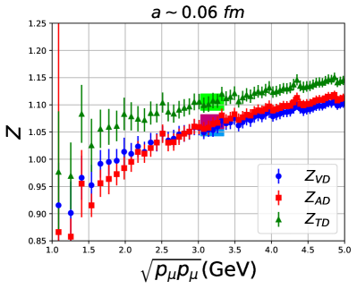
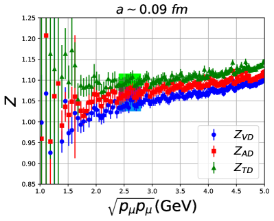
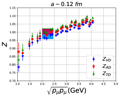
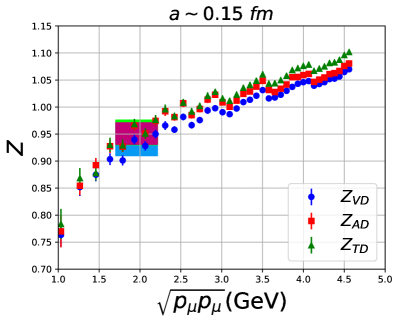
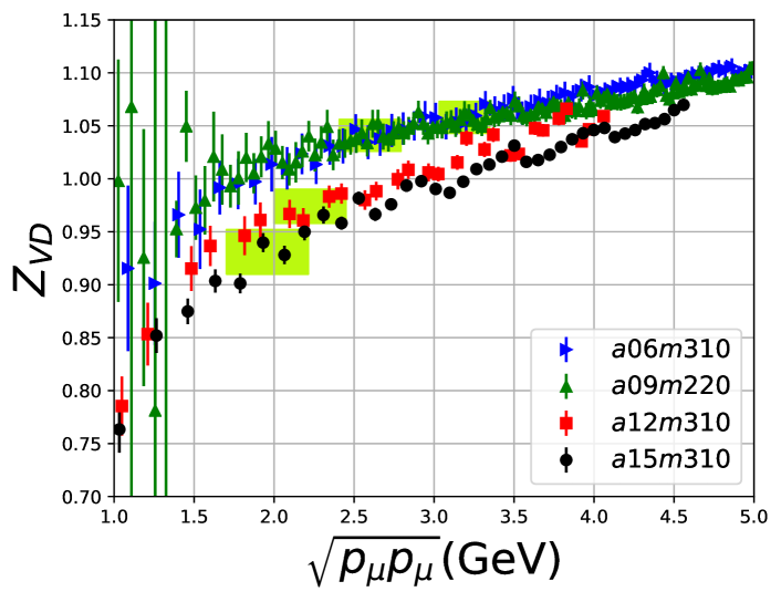
In Fig. 7, we show the behavior of the renormalization factors in the scheme at GeV for the four ensembles as a function of —the scale of the scheme on the lattice. In Fig. 8 we compare , used to renormalize , calculated on four ensembles, one at each lattice spacing.
For all three operators, the data do not show a window in where the results are independent of . The variation in the data is due to a combination of the breaking of full rotational invariance on the lattice and other dependent artifacts. This is the dominant uncertainty and many methods have been proposed to control it, see for example Refs. Harris et al. (2019); Alexandrou et al. (2020a); Bhattacharya et al. (2016). In Ref. Bhattacharya et al. (2016), we explored three methods that gave consistent results, and of these we have selected the strategy labeled “Method B” there as it is the most straightforward. In this approach, we take an average over the data points in an interval of about , where the scale GeV is chosen to be large enough to avoid nonperturbative effects and at which perturbation theory is expected to be reasonably well behaved. Also, this choice satisfies both and in the continuum limit as desired. The window over which the data are averaged and the error (half the height of the band) are shown by shaded bands in Figs. 7 and 8. Noting the large variation with , we take twice this error, ie, full height of the band, for a very conservative error estimate for all three s.
These final estimates of , and used to renormalize the momentum fraction, the helicity moment and the transversity moment, respectively, are given in Table 9.
References
- Brock et al. (1995) R. Brock et al. (CTEQ), Rev. Mod. Phys. 67, 157 (1995).
- Yoon et al. (2017a) B. Yoon, M. Engelhardt, R. Gupta, T. Bhattacharya, J. R. Green, B. U. Musch, J. W. Negele, A. V. Pochinsky, A. Schafer, and S. N. Syritsyn, Phys. Rev. D 96, 094508 (2017a), arXiv:1706.03406 [hep-lat] .
- Diehl (2003) M. Diehl, Generalized parton distributions, Ph.D. thesis (2003), arXiv:hep-ph/0307382 .
- Accardi et al. (2016a) A. Accardi et al., Eur. Phys. J. A 52, 268 (2016a), arXiv:1212.1701 [nucl-ex] .
- Boer et al. (2011) D. Boer et al., (2011), arXiv:1108.1713 [nucl-th] .
- Lin et al. (2018) H.-W. Lin et al., Prog. Part. Nucl. Phys. 100, 107 (2018), arXiv:1711.07916 [hep-ph] .
- Aoki et al. (2020) S. Aoki et al. (Flavour Lattice Averaging Group), Eur. Phys. J. C 80, 113 (2020), arXiv:1902.08191 [hep-lat] .
- Cichy and Constantinou (2019) K. Cichy and M. Constantinou, Adv. High Energy Phys. 2019, 3036904 (2019), arXiv:1811.07248 [hep-lat] .
- Karthik (2019) N. Karthik, “Lattice computations of PDF: Challenges and progress,” https://indico.cern.ch/event/764552/contributions/3420535/attachments/1864018/3064443/LatticeTalk19_NK.pdf (2019), accessed: 2020-05-20.
- Follana et al. (2007) E. Follana et al. (HPQCD Collaboration, UKQCD Collaboration), Phys.Rev. D75, 054502 (2007), arXiv:hep-lat/0610092 [hep-lat] .
- Bazavov et al. (2013) A. Bazavov et al. (MILC Collaboration), Phys.Rev. D87, 054505 (2013), arXiv:1212.4768 [hep-lat] .
- Bhattacharya et al. (2015) T. Bhattacharya, V. Cirigliano, S. Cohen, R. Gupta, A. Joseph, H.-W. Lin, and B. Yoon (PNDME), Phys. Rev. D92, 094511 (2015), arXiv:1506.06411 [hep-lat] .
- Bhattacharya et al. (2016) T. Bhattacharya, V. Cirigliano, S. Cohen, R. Gupta, H.-W. Lin, and B. Yoon, Phys. Rev. D94, 054508 (2016), arXiv:1606.07049 [hep-lat] .
- Gupta et al. (2018) R. Gupta, Y.-C. Jang, B. Yoon, H.-W. Lin, V. Cirigliano, and T. Bhattacharya, Phys. Rev. D98, 034503 (2018), arXiv:1806.09006 [hep-lat] .
- Sheikholeslami and Wohlert (1985) B. Sheikholeslami and R. Wohlert, Nucl. Phys. B259, 572 (1985).
- Hasenfratz and Knechtli (2001) A. Hasenfratz and F. Knechtli, Phys.Rev. D64, 034504 (2001), arXiv:hep-lat/0103029 [hep-lat] .
- Bali et al. (2010) G. S. Bali, S. Collins, and A. Schafer, Comput.Phys.Commun. 181, 1570 (2010), arXiv:0910.3970 [hep-lat] .
- Blum et al. (2013) T. Blum, T. Izubuchi, and E. Shintani, Phys.Rev. D88, 094503 (2013), arXiv:1208.4349 [hep-lat] .
- Gockeler et al. (1996) M. Gockeler, R. Horsley, E.-M. Ilgenfritz, H. Perlt, P. E. L. Rakow, G. Schierholz, and A. Schiller, Phys. Rev. D53, 2317 (1996), arXiv:hep-lat/9508004 [hep-lat] .
- Harris et al. (2019) T. Harris, G. von Hippel, P. Junnarkar, H. B. Meyer, K. Ottnad, J. Wilhelm, H. Wittig, and L. Wrang, Phys. Rev. D100, 034513 (2019), arXiv:1905.01291 [hep-lat] .
- Davoudi and Savage (2012) Z. Davoudi and M. J. Savage, Phys. Rev. D86, 054505 (2012), arXiv:1204.4146 [hep-lat] .
- Detmold and Lin (2006) W. Detmold and C. J. D. Lin, Phys. Rev. D73, 014501 (2006), arXiv:hep-lat/0507007 [hep-lat] .
- Detmold et al. (2018) W. Detmold, I. Kanamori, C. J. D. Lin, S. Mondal, and Y. Zhao, Proceedings, 36th International Symposium on Lattice Field Theory (Lattice 2018): East Lansing, MI, United States, July 22-28, 2018, PoS LATTICE2018, 106 (2018), arXiv:1810.12194 [hep-lat] .
- Bhattacharya et al. (2014) T. Bhattacharya, S. D. Cohen, R. Gupta, A. Joseph, H.-W. Lin, and B. Yoon, Phys. Rev. D89, 094502 (2014), arXiv:1306.5435 [hep-lat] .
- Bali et al. (2014) G. S. Bali, S. Collins, B. Gläßle, M. Göckeler, J. Najjar, R. H. Rödl, A. Schäfer, R. W. Schiel, A. Sternbeck, and W. Söldner, Phys. Rev. D90, 074510 (2014), arXiv:1408.6850 [hep-lat] .
- Bali et al. (2012) G. S. Bali, S. Collins, M. Deka, B. Glassle, M. Gockeler, J. Najjar, A. Nobile, D. Pleiter, A. Schafer, and A. Sternbeck, Phys. Rev. D86, 054504 (2012), arXiv:1207.1110 [hep-lat] .
- Yoon et al. (2016) B. Yoon et al., Phys. Rev. D93, 114506 (2016), arXiv:1602.07737 [hep-lat] .
- Babich et al. (2010) R. Babich, J. Brannick, R. Brower, M. Clark, T. Manteuffel, et al., Phys.Rev.Lett. 105, 201602 (2010), arXiv:1005.3043 [hep-lat] .
- Clark et al. (2010) M. Clark, R. Babich, K. Barros, R. Brower, and C. Rebbi, Comput.Phys.Commun. 181, 1517 (2010), arXiv:0911.3191 [hep-lat] .
- Yoon et al. (2017b) B. Yoon et al., Phys. Rev. D 95, 074508 (2017b), arXiv:1611.07452 [hep-lat] .
- Jang et al. (2020) Y.-C. Jang, R. Gupta, B. Yoon, and T. Bhattacharya, Phys. Rev. Lett. 124, 072002 (2020), arXiv:1905.06470 [hep-lat] .
- Alexandrou et al. (2020a) C. Alexandrou, S. Bacchio, M. Constantinou, J. Finkenrath, K. Hadjiyiannakou, K. Jansen, G. Koutsou, H. Panagopoulos, and G. Spanoudes, (2020a), arXiv:2003.08486 [hep-lat] .
- Alexandrou et al. (2020b) C. Alexandrou et al., Phys. Rev. D 101, 034519 (2020b), arXiv:1908.10706 [hep-lat] .
- Bali et al. (2019) G. S. Bali, S. Collins, M. Göckeler, R. Rödl, A. Schäfer, and A. Sternbeck, Phys. Rev. D 100, 014507 (2019), arXiv:1812.08256 [hep-lat] .
- Yang et al. (2018) Y.-B. Yang, J. Liang, Y.-J. Bi, Y. Chen, T. Draper, K.-F. Liu, and Z. Liu, Phys. Rev. Lett. 121, 212001 (2018), arXiv:1808.08677 [hep-lat] .
- Alexandrou et al. (2017) C. Alexandrou, M. Constantinou, K. Hadjiyiannakou, K. Jansen, C. Kallidonis, G. Koutsou, A. Vaquero Avilés-Casco, and C. Wiese, Phys. Rev. Lett. 119, 142002 (2017), arXiv:1706.02973 [hep-lat] .
- Abdel-Rehim et al. (2015) A. Abdel-Rehim et al., Phys. Rev. D92, 114513 (2015), [Erratum: Phys. Rev.D93,no.3,039904(2016)], arXiv:1507.04936 [hep-lat] .
- Green et al. (2014) J. R. Green, M. Engelhardt, S. Krieg, J. W. Negele, A. V. Pochinsky, and S. N. Syritsyn, Phys. Lett. B734, 290 (2014), arXiv:1209.1687 [hep-lat] .
- Aoki et al. (2010) Y. Aoki, T. Blum, H.-W. Lin, S. Ohta, S. Sasaki, et al., Phys.Rev. D82, 014501 (2010), arXiv:1003.3387 [hep-lat] .
- Bratt et al. (2010) J. Bratt et al. (LHPC Collaboration), Phys.Rev. D82, 094502 (2010), arXiv:1001.3620 [hep-lat] .
- Hou et al. (2019) T.-J. Hou et al., (2019), arXiv:1912.10053 [hep-ph] .
- Ethier et al. (2017) J. Ethier, N. Sato, and W. Melnitchouk, Phys. Rev. Lett. 119, 132001 (2017), arXiv:1705.05889 [hep-ph] .
- Ball et al. (2017) R. D. Ball et al. (NNPDF), Eur. Phys. J. C77, 663 (2017), arXiv:1706.00428 [hep-ph] .
- Alekhin et al. (2017) S. Alekhin, J. Blümlein, S. Moch, and R. Placakyte, Phys. Rev. D96, 014011 (2017), arXiv:1701.05838 [hep-ph] .
- Accardi et al. (2016b) A. Accardi, L. T. Brady, W. Melnitchouk, J. F. Owens, and N. Sato, Phys. Rev. D93, 114017 (2016b), arXiv:1602.03154 [hep-ph] .
- Abramowicz et al. (2015) H. Abramowicz et al. (H1, ZEUS), Eur. Phys. J. C75, 580 (2015), arXiv:1506.06042 [hep-ex] .
- Dulat et al. (2016) S. Dulat, T.-J. Hou, J. Gao, M. Guzzi, J. Huston, P. Nadolsky, J. Pumplin, C. Schmidt, D. Stump, and C. P. Yuan, Phys. Rev. D93, 033006 (2016), arXiv:1506.07443 [hep-ph] .
- Harland-Lang et al. (2015) L. A. Harland-Lang, A. D. Martin, P. Motylinski, and R. S. Thorne, Eur. Phys. J. C75, 204 (2015), arXiv:1412.3989 [hep-ph] .
- Nocera et al. (2014) E. R. Nocera, R. D. Ball, S. Forte, G. Ridolfi, and J. Rojo (NNPDF), Nucl. Phys. B887, 276 (2014), arXiv:1406.5539 [hep-ph] .
- de Florian et al. (2009) D. de Florian, R. Sassot, M. Stratmann, and W. Vogelsang, Phys. Rev. D80, 034030 (2009), arXiv:0904.3821 [hep-ph] .
- de Florian et al. (2008) D. de Florian, R. Sassot, M. Stratmann, and W. Vogelsang, Phys. Rev. Lett. 101, 072001 (2008), arXiv:0804.0422 [hep-ph] .
- Edwards and Joo (2005) R. G. Edwards and B. Joo (SciDAC, LHPC, UKQCD), Nucl. Phys. B Proc. Suppl. 140, 832 (2005), arXiv:hep-lat/0409003 .
- Gockeler et al. (2010) M. Gockeler et al., Phys. Rev. D82, 114511 (2010), [Erratum: Phys. Rev.D86,099903(2012)], arXiv:1003.5756 [hep-lat] .
- Constantinou et al. (2013) M. Constantinou, M. Costa, M. Göckeler, R. Horsley, H. Panagopoulos, H. Perlt, P. E. L. Rakow, G. Schierholz, and A. Schiller, Phys. Rev. D87, 096019 (2013), arXiv:1303.6776 [hep-lat] .
- Gracey (2003) J. A. Gracey, Nucl. Phys. B667, 242 (2003), arXiv:hep-ph/0306163 [hep-ph] .