MOJAVE XX. Persistent Linear Polarization Structure in Parsec-scale AGN Jets
Abstract
We analysed the parsec-scale linear polarization properties of 436 active galactic nuclei (AGN) based on 15 GHz polarimetric Very Long Baseline Array (VLBA) observations. We present polarization and total intensity images averaged over at least five epochs since 1996 January 19 through 2019 August 4. Stacking improves the image sensitivity down to 30 Jy beam-1 and effectively fills out the jet cross-section both in total intensity and linear polarization. It delineates the long-term persistent magnetic field configuration and its regularity by restoring spatial distributions of the electric vector position angle (EVPA) and fractional polarization, respectively. On average, about ten years of stacking period is needed to reveal the stable and most-complete polarization distribution of a source. We find that the degree of polarization significantly increases down and across the jet towards its edges, typically manifesting U or W-shaped transverse profiles, suggesting a presence of a large-scale helical magnetic field associated with the outflow. In some AGN jets, mainly BL Lacs, we detect quasi-constant fractional polarization profiles across the jet, accompanied by EVPAs that closely follow the outflow. BL Lacs show higher fractional polarization values in their cores and jets than those in quasars up to hectoparsec de-projected scales, while on larger scales, they become comparable. High-synchrotron-peaked BL Lac jets are found to be less polarized than intermediate and low-synchrotron-peaked BL Lacs. The spatial distribution of the EVPAs in BL Lacs tend to align with the local jet direction, while quasars show an excess of orthogonal polarization orientation.
keywords:
quasars: general – BL Lacertae objects: general – galaxies: active – galaxies: jets – radio continuum: galaxies – polarization1 Introduction
Active galactic nuclei (AGN) are the most powerful non-transient sources in the Universe. Their centers host supermassive black holes (SMBH). It is widely accepted that bi-polar antiparallel outflows are launched as a result of the accretion of matter on an SMBH, with the extraction of energy and angular momentum from the rotating central machine (Blandford & Znajek, 1977) and/or accretion disk (Blandford & Payne, 1982). Simulations show that the most efficient outflows are produced if spins of the SMBH and accretion disk are prograde (Tchekhovskoy & McKinney, 2012). AGN jets emit radiation over the entire electromagnetic spectrum, from radio to GeV–TeV gamma rays. Recently, evidence was found that radio-bright blazars are the sources of high-energy astrophysical neutrinos (e.g. Plavin et al., 2020, 2021; Hovatta et al., 2021; Buson et al., 2022, see also discussion in Zhou et al. 2021 and Plavin et al. 2022).
The jets propagate through the ambient medium, which is a factor of – times more dense than the jet (Martí, 2019). Changes in the ISM pressure profile form a series of quasi-stationary recollimation shocks in the jet predicted by theory, at least for super-magnetosonic jets (Meier, 2011; Mizuno et al., 2015) and also detected with very long baseline interferometry (VLBI) observations as slow pattern speed components in the inner jet regions, mainly within 3–4 pc projected distance from the radio core (Cohen et al., 2014; Jorstad et al., 2017; Lister et al., 2019). The outflows initially have a quasi-parabolic shape (Vlahakis & Königl, 2003; Beskin & Nokhrina, 2006; Komissarov et al., 2007) and undergo a transition to quasi-conical geometry at distances of – gravitational radii, most likely due to a change from magnetically dominated to an equipartition regime, as found for a dozen of nearby () AGN for which VLBI provides high enough linear resolution (Asada & Nakamura, 2012; Pushkarev et al., 2017; Kovalev et al., 2020). Post-recollimation-shock(s) jet features are superluminal, with apparent speeds up to 40 (Jorstad et al., 2005; Piner et al., 2012; Lister et al., 2021) showing signatures of residual acceleration up to the de-projected distances of 100 pc, beyond which the outflows either manifest a constant speed regime or start to decelerate (Homan et al., 2015).
The key agent in forming, accelerating and collimating the relativistic jets is the magnetic field originally threaded through the accretion disc and then propelled out and wound up in the outflow. An indication for a toroidal component to the magnetic field in a number of transversely resolved AGN jets was found, as evident from the gradients of Faraday rotation measure across the outflow (e.g. Asada et al., 2002; Zavala & Taylor, 2005; Hovatta et al., 2012; Zamaninasab et al., 2013; Gabuzda et al., 2015; Kravchenko et al., 2017). Toroidal magnetic fields imply that a current flows in the jet, with the expected values in a range of – A (Wardle, 2018). On the other hand, high variability in the flux and linear polarization of AGN jets suggests the presence of shocks and plasma turbulence, so that the magnetic field is partly disordered being a combination of regular and chaotic magnetic field components (Marscher, 2014; Marscher et al., 2017). In this paper, we study the stable component of the magnetic field of AGN jets, its regularity and configuration by constructing and analysing fractional polarization and electric vector position angle (EVPA) distributions averaged over the available epochs of VLBA observations. In the companion paper, Zobnina et al. (2022) based on the same observational data, we investigated the decade-long variability of the linear polarization of parsec-scale AGN outflows.
The layout of the paper is as follows. In section 2, we describe our observational data and the properties of the studied AGN jet sample. We discuss our method of constructing stacked maps in total intensity and linear polarization in section 3 and present the statistics of the images. We present our results in section 4 and summarize the main conclusions in section 5. By the term ‘core’ we mean the apparent origin of AGN jets, which is typically seen as the brightest and most compact feature in VLBI images of blazars (e.g. Lobanov, 1998). The spectral index is defined as , where is the flux density measured at frequency . All position angles are given in degrees east of north. We adopt a cosmology with , and km s-1 Mpc-1 (Komatsu et al., 2009).
2 Observational data and source sample
For the purposes of our study, we selected sources that have at least five polarization-sensitive observing epochs with the VLBA at 15 GHz. Over 90 per cent of the observations were performed within the MOJAVE program111https://www.cv.nrao.edu/MOJAVE, while the rest were taken from the NRAO archive. We excluded the quasar 2023+335, which is subject to refractive-dominated scattering (Pushkarev et al., 2013) resulting in the unclear position of the core component in a number of observing epochs. The quasar 1329126 initially having five epochs was also dropped as one epoch had poor data quality. Thus, our sample comprises 436 sources listed in Table 1, 207 of which are members of the MOJAVE 1.5 Jy quarter-century (QC) flux-density limited sample (Lister et al., 2021) containing 232 objects. Four epochs of 0316+413 prior to 1999 December 27 were excluded due to the unclear core position of the source. Overall, we have 5921 single-epoch maps at 368 unique observational epochs between 1996 January 19 to 2019 August 4.
The sources in the MOJAVE program are observed with individual cadence determined by the rate of the corresponding morphological changes. The distribution of the median time separation of the neighbouring epochs for the 436 sources from our sample is wide (Figure 1), ranging from 38 days for the most frequently observed source, BL Lacertae object 0716+714, to 861 days for the radio galaxy 1345+125. The median cadence for the whole sample is six months.
Additional details on the source sample, including time coverage, redshift, optical and SED class distributions, are provided in the companion paper by Zobnina et al. (2022). The data reduction, the process of single-epoch imaging and structure model fitting are described in Lister et al. (2009); Lister et al. (2018).

| B1950.0 name | J2000.0 name | Alias | Opt. class | MOJAVE 1.5 | LAT | Spectrum | References | |
|---|---|---|---|---|---|---|---|---|
| (1) | (2) | (3) | (4) | (5) | (6) | (7) | (8) | (9) |
| 0003066 | J00060623 | NRAO 005 | 0.3467 | B | Y | Y | LSP | Jones et al. (2005),2 |
| 0003380 | J00053820 | S4 0003+38 | 0.229 | Q | N | Y | LSP | Stickel & Kuehr (1994),1 |
| 0006061 | J00090628 | TXS 0006+061 | … | B | N | Y | LSP | Rau et al. (2012),1 |
| 0007106 | J00101058 | III Zw 2 | 0.0893 | G | Y | Y | LSP | Sargent (1970),3 |
| 0010405 | J00134051 | 4C +40.01 | 0.256 | Q | N | Y | LSP | Thompson et al. (1992),2 |
| 0011189 | J00131910 | RGB J0013+191 | 0.477 | B | N | Y | LSP | Shaw et al. (2013),2 |
| 0012610 | J00146117 | 4C +60.01 | … | U | N | Y | LSP | …,1 |
| 0014813 | J00178135 | S5 0014+813 | 3.382 | Q | N | N | LSP | Varshalovich et al. (1987),3 |
| 0015054 | J00170512 | PMN J0017-0512 | 0.226 | Q | N | Y | LSP | Shaw et al. (2012),1 |
| 0016731 | J00197327 | S5 0016+73 | 1.781 | Q | Y | Y | LSP | Lawrence et al. (1986),2 |
-
•
Columns are as follows: (1) Source name in B1950.0 coordinates; (2) Source name in J2000.0 coordinates; (3) Alias; (4) Redshift; (5) Optical Class (Q=quasar, B=BL Lac, G=radio galaxy, N=narrow-line Seyfert 1, U=unknown); (6) Member of the MOJAVE 1.5 Jy QC Sample (Y = yes, N = no); (7) Fermi LAT-detected; (8) SED Class (LSP/ISP/HSP = Low/Intermediate/High Synchrotron Peaked); (9) References for Redshift/Optical and SED Classification. SED property references are as follows: 1 = Ackermann et al. (2015), 2 = Ajello et al. (2020), 3 = Stratta et al. (2011), 4 = Meyer et al. (2011), 5 = Xiong et al. (2015), 6 = Chang et al. (2017), 7 = Nieppola et al. (2008), 8 = Ajello et al. (2017), 9 = Ackermann et al. (2011), 10 = Abdo et al. (2009b), 11 = Nieppola et al. (2006), 12 = Chang et al. (2019), 13 = Abdo et al. (2009a), and 14 = Hervet et al. (2015). (This table is available in its entirety in a machine-readable form as supplementary material and at the CDS VizieR.)
3 Total intensity and linear polarization stacked images
To produce a stacked map in total intensity, we performed the following steps. First, every single-epoch image was shifted such that the core component, whose position is determined from the structure model fitting and assumed to be stable (though small non-zero shifts caused by the emergence of new components are possible), was placed at the phase centre of the map. Second, the source brightness distribution represented by the CLEAN components was convolved with a circular restoring beam, the full width at half maximum (FWHM) of which in milliarcseconds is the average between
| (1) |
and
| (2) |
where is the source J2000 declination in degrees, Equation 1 and Equation 2 are the spline fits to the maximum and minimum FWHM dimensions of the naturally weighted elliptical restoring beam for several thousand 15 GHz VLBA observations made within the MOJAVE program. Thereafter, all single-epochs maps were averaged to make a stacked image .
As for the polarization stacking, there are two possible methods. First, used in this paper, is to follow the same procedure as for Stokes I but for Stokes Q and U, and then produce stacked maps of linearly polarized intensity , fractional polarization and its direction . This approach treats polarization as a vector. An alternative method, applied in Zobnina et al. (2022) is based on making single-epoch polarization maps first and then taking their scalar mean (regardless of EVPA) to derive typical values, e.g. to study variability.
Following Wardle & Kronberg (1974), we corrected the stacked maps for the Ricean bias, i.e. . The corrections are per cent for the regions above the lowest polarization contour drawn at the level, where was estimated as
| (3) |
where , as the noise statistics of the map in a sky region, which either blank or having a low signal-to-noise ratio, follow a Rayleigh distribution. In turn, was calculated using the following procedure: (i) for each outer quadrant of the map (with a square of 1/16 of a total image), the rms level is calculated, (ii) the highest rms value is removed and (iii) the median over three remaining rms estimates is taken. The estimations of uncertainty in , , EVPA and polarization feed leakage derived from the simulations and analytical expressions are discussed in Appendix A.
Finally, we corrected the total and linear polarization intensity distributions for the CLEANing bias (Appendix B). After subtracting the -bias, we show only positive values of polarization intensity and corresponding fractional polarization. This is justified as (i) fewer than 1 per cent of all pixels with presented in the stacked images are negative, i.e. and (ii) fewer than 1 per cent of the negative -pixels are significantly (at level) different from zero.
We also filtered out epochs with poor data quality. If the noise level of a single-epoch total intensity map exceeded three times the corresponding median rms for a given source, the epoch was excluded. In total, we ruled out 65 noisy maps (about 1 per cent of the total number) from 31 sources. This additionally increased the dynamic range of the stacked images by a factor up to a few, especially in the cases with a small number of the observing epochs.
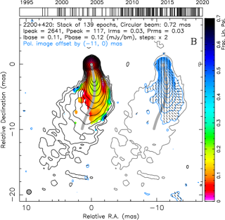
In Figure 2, we show the examples of the stacked maps having the minimum (5), median (9), maximum (139) number of epochs, and also a source which is unpolarized. For each object, two plots are given: total intensity contours overlaid with a distribution of fractional linear polarization and blue linear polarization contours shifted aside and overlaid with ticks of an arbitrary fixed length representing electric vectors. Their directions have not been corrected for Faraday rotation, which is typically at a level of a few degrees at 15 GHz in the inner jet regions, as found in our earlier rotation measure study of the MOJAVE sample (Hovatta et al., 2012). We list the parameters of the stacked images in Table 2.
We analyzed the influence of the moving jet components on the stacked maps by comparing (i) a distance they propagate down the jet, , where is the maximum proper motion (Lister et al., 2021) and is the time interval between the first and last observing epoch and (ii) a typical separation between the components derived individually for 398 sources. A median ratio indicates that the moving components substantially affect the -stacked maps, making them smoother along the outflow. Only about 25 per cent of the stacked maps are not essentially influenced by the moving jet features (), due to either their low proper motion and limited time interval (e.g. in the quasar 1550582) or due to a large separation between the components (e.g. in the radio galaxy 1345125). The influence of the moving jet features on the polarization stacked maps is not that straightforward and might depend on the nature of the bright components. For instance, the jet magnetic field may be turbulent or weakly anisotropic with modest shear causing a net longitudinal field. If the moving components are shocks that compress the magnetic field transverse to the jet (Laing, 1980; Hughes et al., 1985), then their polarization will be orthogonal to that of the underlying jet, dominating the apparent polarization if the number and strength of the components is high. If the jet features are plasmoids with random magnetic field, their role would be unimportant. We discuss it further in subsection 4.5 based on the inferred EVPA patterns.


| Source | First Epoch | N | Beam | |||||
|---|---|---|---|---|---|---|---|---|
| (yyyy-mm-dd) | (yr) | (mas) | (mJy bm-1) | (mJy bm-1) | (mJy bm-1) | (mJy bm-1) | ||
| (1) | (2) | (3) | (4) | (5) | (6) | (7) | (8) | (9) |
| 0003066 | 2003-02-05 | 9.74 | 18 | 0.93 | 1242.8 | 83.0 | 0.11 | 0.05 |
| 0003380 | 2006-03-09 | 7.42 | 10 | 0.73 | 462.1 | 3.4 | 0.06 | 0.06 |
| 0006061 | 2011-12-29 | 1.43 | 5 | 0.88 | 149.6 | 6.5 | 0.07 | 0.07 |
| 0007106 | 2004-02-11 | 9.31 | 13 | 0.86 | 869.3 | 3.0 | 0.05 | 0.05 |
| 0010405 | 2006-04-05 | 5.22 | 12 | 0.72 | 508.1 | 3.2 | 0.06 | 0.05 |
| 0011189 | 2013-12-15 | 2.22 | 8 | 0.82 | 107.9 | 3.5 | 0.02 | 0.02 |
| 0012610 | 2017-01-03 | 2.48 | 6 | 0.66 | 214.2 | 1.0 | 0.04 | 0.03 |
| 0014813 | 2016-09-26 | 2.75 | 11 | 0.67 | 381.7 | 17.0 | 0.03 | 0.03 |
| 0015054 | 2009-07-05 | 4.01 | 8 | 0.92 | 240.6 | 2.8 | 0.05 | 0.04 |
| 0016731 | 2003-08-28 | 15.79 | 8 | 0.66 | 1390.7 | 13.8 | 0.07 | 0.07 |
-
•
Columns are as follows: (1) Source name in B1950.0 coordinates; (2) Date of first epoch; (3) Time range between first and last epochs; (4) Number of single-epoch maps in stack; (5) FWHM of restoring beam; (6) -map peak; (7) -map peak; (8) -map noise level; (9) -map noise level.
(This table is available in its entirety in a machine-readable form as supplementary material and at the CDS VizieR.)
3.1 Unpolarized sources
There are 23 (5.3 per cent of the sample) essentially unpolarized sources (Table 3) at the sensitivity level of our stacked images. Eleven of them are radio galaxies, making up 46 per cent fraction of this source spectral type in the sample. One of these radio galaxies, 0055+300, is shown in Figure 2 (bottom right). Four of the radio galaxies, 0128+554, 1404+286, 1509+054 and 2021+614, are classified as compact symmetric objects (CSO). Our sample has one more CSO, i.e. the GPS radio galaxy 1345+125. Polarization emission in this source is detected in the southern jet feature, at about 45 mas from the core (Lister et al., 2003). However, the integrated fractional polarization over the entire source is relatively low, per cent. Unpolarized quasars and BL Lacs are much more rare, both represented by six sources, which makes 2 and 4 per cent of their fractions, respectively. For one of these quasars, 0710+196, polarization is detected in the core at most of the observing epochs, two of which, 2009 August 19 and 2014 January 25, show the strongest polarization with comparable flux but roughly orthogonal EVPA directions, thereby canceling each other in vector averaging and resulting in close to zero stacked . Another quasar, 1722+401, demonstrates similar behaviour, with nearly perpendicular EVPAs at the first two and last two epochs. Two BL Lacs, 0329654 and 2013092, are the weakest sources in our sample, making detection of their polarization unlikely due to a sensitivity limit. Taking this into account, only 1 per cent of the quasars and 3 per cent of the BL Lacs from our sample are unpolarized. Some sources, e.g. 0615172 and 2021614, show faint and most likely spurious polarization in their stacked -maps due to the -signal being detected at one epoch only, which can be a result of poor leakage term solutions. We excluded these 23 sources from our further analysis.
The reason why some sources of different optical classes, redshifts, apparent speeds and viewing angles are so weakly polarized is unclear. Their polarization sensitivity reached both in single-epoch and stacked images is comparable to that of other AGNs in our sample. It is possible that the weakly polarized sources are subject to strong Faraday depolarization by an external screen associated with an obscuring torus due to large viewing angles of their jets, which is typically the case for radio galaxies (e.g. Aller et al., 2003; Middelberg et al., 2005). Internal plasma processes might also play a role, e.g. if a turbulent component of magnetic field in a jet dominates the ordered component on small scales (Marscher, 2014). In this scenario, the chaotic directions of magnetic field effectively cancel out polarization. It is further supported by a significantly higher fraction (almost every second object) of weakly polarized radio galaxies compared to that of blazars, as we probe the outflows on smaller (de-projected) linear separations from the true jet origin, where turbulence is expected to be stronger, and Faraday rotation could be higher because of denser thermal plasma.
| Source | Op. cl. | N | |||
| (mJy) | (mJy) | ||||
| (1) | (2) | (3) | (4) | (5) | (6) |
| 0055300 | G | 0.0165 | 6 | 664.5 | 2.42 |
| 0128554a | G | 0.0365 | 6 | 105.6 | 1.88 |
| 0238084 | G | 0.0050 | 24 | 1085.9 | 0.66 |
| 1128047 | G | 0.266 | 10 | 698.2 | 1.24 |
| 1404286a | G | 0.077 | 8 | 819.9 | 2.75 |
| 1509054a | G | 0.084 | 8 | 582.3 | 1.75 |
| 1637826 | G | 0.024 | 10 | 803.4 | 1.86 |
| 1833326 | G | 0.0579 | 8 | 172.1 | 0.92 |
| 1845797 | G | 0.0555 | 13 | 439.9 | 1.92 |
| 1957405 | G | 0.0561 | 9 | 1437.9 | 2.82 |
| 2021614a | G | 0.227 | 12 | 2212.1 | 3.84 |
| 0646600 | Q | 0.455 | 7 | 742.4 | 2.55 |
| 0710196b | Q | 0.54 | 10 | 222.0 | 2.56 |
| 0742103 | Q | 2.624 | 13 | 1354.5 | 1.45 |
| 1722401b | Q | 1.049 | 5 | 588.7 | 1.96 |
| 2031216 | Q | 0.1735 | 5 | 304.4 | 0.72 |
| 2043749 | Q | 0.104 | 7 | 263.0 | 0.90 |
| 0111021 | B | 0.047 | 7 | 505.7 | 1.69 |
| 0329654c | B | … | 7 | 63.4 | 1.78 |
| 0615172 | B | 0.098 | 5 | 159.7 | 0.52 |
| 1413135 | B | 0.247 | 12 | 954.3 | 4.11 |
| 2013092c | B | … | 6 | 52.1 | 1.62 |
| 2047098 | B | 0.226 | 6 | 566.5 | 1.80 |
-
•
Columns are as follows: (1) Source name; (2) Optical class: quasar (Q), BL Lac (B), radio galaxy (G); (3) Redshift; (4) Number of single-epoch maps in stack; (5) Total cleaned Stokes flux density in the stacked 15 GHz VLBA image; (6) Total linear polarization flux density derived from the stacked Stokes and maps as .
aCompact symmetric object.
bSinge-epoch polarization detected in the core.
cWeak in total intensity.
3.2 Integrated polarization
We derived the integrated fractional polarization over the entire source as , where and are the total flux density and polarized flux, respectively, calculated over the image above the corresponding and levels. The values of are distributed in a wide range, from 0.06 per cent for the galaxy NGC 1052 to 17.6 per cent for the quasar 3C 119. The distributions of for the sources of different optical classes are shown in Figure 3. The least polarized sources are radio galaxies, with a median per cent. According to a Kolmogorov-Smirnov test, quasars and BL Lacs have statistically different distributions, with the medians of equal to and per cent, respectively. BL Lacs being devided into different SED classes show that HSP sources are on average less polarized than ISP and LSP BL Lacs (Figure 4).


3.3 Total intensity ridgelines
We traced out the total intensity ridgeline for each stacked map, following the approach described in Pushkarev et al. (2017). It is based on making an azimuthal slice around the core component at a given radius and finding a position of the weighted average in total intensity. The starting ridgeline point coincides with the core position and then the algorithm advances downstream for successively increasing core separations with a step of 0.5 mas, skipping the regions where emission is too faint, . After that we applied a cubic spline interpolation to have a ridgeline point approximately every 0.1 mas along the ridgeline. In the cases when the counter-jet is detected, i.e. in the radio galaxies TXS 0128+554, NGC 1052, 3C 84, PMN J1511+0518, Cygnus A, quasar S4 0646+60 and BL Lac PKS B1413+135, we show the ridgeline for the approaching, brighter jet.
4 Polarization properties along and across jets
4.1 Fractional polarization
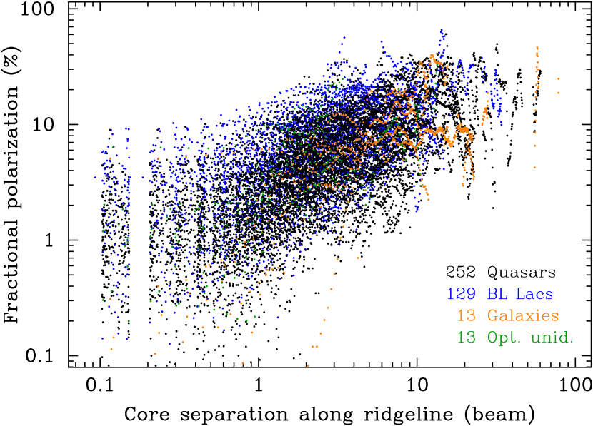
The first evidence that the degree of linear polarization of distinct jet features increases with their separation from the core was reported by Cawthorne et al. (1993), who analysed polarimetric VLBI data at 5 GHz for a small sample of AGN jets. Later, this trend was also detected at 22 and 43 GHz (Lister & Smith, 2000; Lister, 2001) for samples of 18 and 32 sources, respectively. At 15 GHz, the trend was found by Lister & Homan (2005), who studied the first-epoch MOJAVE data for the flux-density-limited complete sample of 133 sources. This observational result implies that the magnetic field, decreasing with distance from the true jet vertex as ( for the case of the poloidal field and for the toroidal field and a conical jet shape), becomes more ordered, if it is not entirely caused by, e.g. decreasing depolarization along the jet.
In Figure 5, we show the dependence of fractional polarization as a function of the projected, i.e. observed, distance down the jet along its ridgeline for the largest ever sample of over 400 sources. We confirm the general increase in downstream and discuss its features. First, the degree of linear polarization in the core region (within 0.5 beam) ranges from about 0.1 per cent to 10 per cent, with a median of about 1 per cent and 2 per cent for quasars and BL Lacs, respectively, whereas the radio galaxy cores are found to be low or completely unpolarized. The synchrotron emission of the core is partially opaque, leading to a further decrease in the fractional polarization both through opacity and possibly increased Faraday effects if they are present. The low values are also caused by in-beam depolarization in the case of superposition from polarized emission of unresolved features with different EVPAs.
Beyond the core in the inner jet, increases quite rapidly, mostly due to a switch to an optically thin regime of synchrotron radiation and weakening of the beam depolarization effect. In the outer jet regions, the degree of polarization, on average, continues to grow with distance from the core. This can be explained by weakening shocks and accompanied turbulence of emitting plasma (Marscher, 2014), progressively smaller Faraday rotation (Hovatta et al., 2012; Kravchenko et al., 2017) and the spectral ageing effect (Kardashev, 1962). In the latter phenomenon, the high-energy electrons lose energy faster owing to synchrotron emission. This leads to steepening of both the energy and flux density spectra in the more remote jet parts. VLBI observations showed that the magnitude of the spectral ageing effect is about for parsec-scale AGN jets (Pushkarev & Kovalev, 2012; Hovatta et al., 2014). In turn, this results in the growth of because for the optically thin regime of synchrotron radiation from a region with an ordered magnetic field and randomly oriented pitch angles of relativistic electrons the corresponding maximum of is limited by (Pacholczyk, 1970), where is the power-law index in the energy spectrum of emitting particles .

The growth of fractional polarization down the jet can also occur either through shear in a boundary layer (e.g. Laing & Bridle, 2014) or as the pitch of a helical magnetic field decreases with distance from the origin (Porth et al., 2011). As shown by Butuzova & Pushkarev (2022), the -values on the jet axis gradually increase with decreasing the pitch angle, starting from about . This was derived from modelling transverse slices of fractional polarization for a wide space of geometric and kinematic jet parameters, e.g. the viewing angle ranging from to in the observer’s frame and Doppler factors varying from 4 to about 15. This mechanism, likely contributing insignificantly in the innermost jet parts, can progressively add to the slow logarithmic increase in and ultimately dominate on large scales. The continuous growth in fractional polarization with the core separation, together with close alignment of EVPA with the local jet direction (typically seen in BL Lacs, more in subsection 4.5), allows us to argue for a large-scale ordered component, i.e. helical magnetic field rather than the presence of an isolated jet feature with high fractional polarization (e.g. Pushkarev & Gabuzda, 2000).
We also analysed individual dependencies of along the ridgelines. To get rid of a neighbouring-pixel dependence in a map arising due to convolution with the restoring beam, we interpolated the cubic spline of the ridgeline with a step of half a beam size. For the sources which had five or more such ridgeline points with beyond the core region, we calculated the Kendall’s correlation coefficient (Figure 6). In total, 215 sources satisfied these criteria, 87 of which show significant (with random chance probability , hatched area) positive correlation, while only two objects, 0509+406 and 0603+476, have negative correlation.
As seen in Figure 5, the ridgeline -values of BL Lacs at a given projected distance from the core are typically higher than those of quasars. This confirms earlier results obtained by Lister (2001) on a smaller source sample. To investigate it further, we first converted the angular distances to a linear projected scale for the sources with known redshifts and then corrected for projection by applying the viewing angles derived from the estimates of Doppler factors (Homan et al., 2021) and apparent jet speeds (Lister et al., 2021). The ridgeline -values beyond the one-beam core region of 52 BL Lacs and 211 quasars vs de-projected distance in parsecs are given in Figure 7. It shows that the jet-axis fractional polarization of BL Lacs probed on smaller scales (up to decaparsecs) are considerably higher than those in quasars, but the corresponding slope is flatter, thus intersecting the steeper quasar trend on hectoparsec scales, showing comparable -values. This can be explained by higher rotation measures (Hovatta et al., 2012) or initially larger helical B-field pitch angle or higher rates of energy losses in quasars compared to those of BL Lacertae objects. The HSP (17), ISP (9) and LSP (25) BL Lacs are characterised by on average decreasing viewing angles as found by Homan et al. (2021) and also increasing redshifts. They form different partly overlaid segments of the whole -trend, showing generally higher fractional polarization of LSP BL Lacs. If we compare quasars and LSP BL Lacs which have matched redshifts , there is no systematic difference in fractional polarization along their jet ridgelines.


4.2 Polarization intensity peak position
The brightness distribution of AGN jets on parsec scales in total intensity is typically dominated by a bright core for the sources of all optical classes. It is not the case for linearly polarized emission. Thus, the cores and innermost jet regions of radio galaxies are often unpolarized, and the median -peak position is about 3 mas away from the apparent jet origin (Figure 8). BL Lacs and quasars have their polarization intensity peaks much closer to the core, at a median distance of about 0.2 mas downstream the jet. The non-zero offset is caused by opacity effects in the core region, so that polarization is dominated by the innermost jet components, the emission of which becomes optically thin. The -peak position coincides with the core within the pixel size of 0.1 mas in only 6 per cent of cases for quasars and BL Lacs and none for radio galaxies.
Quasars are found to be strongest in polarization intensity, while BL Lacs have an almost two times weaker median peak, and radio galaxies are about an order of magnitude weaker. However, we remind that in terms of fractional polarization, the BL Lacs are stronger in the core. There are a few exceptional cases when quasars, like radio galaxies, do not reveal any polarization in the core but show a high SNR emission in another jet part. These are 1602+576 with the only polarized feature at about 5 mas from the core, 0821+621 and 1435+638 with detected polarization beyond the core, at separations of about 1 mas. Interestingly, no BL Lacs show such a phenomenon.
4.3 EVPA and jet direction
Earlier, studying the core polarization properties, we found that the EVPAs in the VLBI cores of BL Lacs are better aligned with the innermost jet direction and less variable than in quasars (Hodge et al., 2018). Here, we analyse the EVPA orientation with respect to the local jet direction along the ridgeline. In Figure 9, we plot two-dimensional histograms of vs core distance separately for different optical classes of the sources. BL Lacs do show a tendency for EVPA to follow the jet. It is clearly seen in about 60 per cent of BL Lacs. This confirms earlier results taken by Gabuzda et al. (2000) on the polarized core and jet components from a sample of 24 BL Lacertae objects. The offset of the density peak of the unsigned EVPA deviations from zero is likely caused by a limited accuracy of the local jet direction from ridgelines and noise error on the EVPAs, rather being a real physical effect. Indeed, if the sign of EVPA deviation is taken into account the density peak spreads around zero nearly symmetrically. Only 14 objects (10 per cent) currently classified as BL Lacs, namely, 0141268, 0214083, 0313411, 0518211, 0723008, 0735178, 0845068, 0851202, 1011496, 1133704, 1215303, 1219285, 1514241, 2010463, manifest EVPA roughly orthogonal to the jet direction. If we divide BL Lacs into SED classes, the sources with the aligned EVPA are fractionally distributed very much close to the whole BL Lac sub-sample (55 per cent of LSP, 26 per cent of ISP, and 26 per cent of HSP). However, those characterised by the EVPA transverse to the local jet position angle have a roughly double relative excess of HSP and the corresponding lack of ISP sources. About 26 per cent of BL Lacs show either non-monotonic orientation of EVPA along the jet or reveal polarization in the core region only, with EVPA not aligned with the jet. Some of these sources might represent EVPA aligned with the innermost jet direction if the outflow is bent there but not resolved. The remaining 4 per cent (six sources) are unpolarized objects, listed in Table 3.
The in quasars show all possible values, with a clear predominance of a peak near and a weaker secondary peak at values close to , in contrast to BL Lacs. There is also an indication that EVPAs in quasars and radio galaxies become preferentially transverse to the jet in the outer ridgeline regions. This analysis suggests that might be a good discriminator between flat-spectrum radio quasars and BL Lacertae objects.
4.4 Cumulative stacking
We also produced a series of all intermediate stacked maps for every source by successively adding all available later epochs to the first one to analyse the changes in the image parameters. As expected, the noise level both in and reduces the following dependency (Figure 10, top). The evolution of against the time interval of epochs in a stacked map is shown in Figure 10 (bottom). The noise reaches values down to about 30 Jy beam-1. The three stripes from upper to mid and lower reflect observations carried out with initially different bit-rates of 128 (until mid-2007, brighter sources), 512 and 2048 Mb s-1 (since 2014, weaker sources). Stacking reduced the rms noise by a factor of a few for most cases and up to ten times for the most frequently observed sources. The corresponding dependencies for look qualitatively similar.


In our earlier study of jet shapes and their opening angles (Pushkarev et al., 2017), we found that the apparent jet opening angle increases if more epochs are added to the stacked map. This growth is not monotonic, it plateaus on scales of about five years, implying that stacking revealed a full cross-section of the inner jet. In the current paper, we analyse the effect of stacking on linearly polarized emission. Combining data of different epochs results in higher image sensitivity, enlarging the areas of the revealed jet structure in total and linearly polarized intensity, and , where is the area within the bottom () total intensity contour and is the area within an overlap of the bottom linearly polarized () and total intensity () contours. Thus, the image -filling factor of a jet defined as is limited by 1. In addition to the number of epochs in a stack, their temporal spacing also matters. If the time interval between the first and last epoch is wide enough it allows reaching the maximum value. Figure 11 presents the corresponding jet -filling factor. It increases with up to a certain level, which is distributed in a wide range, with a typical value of about 1/3 and then becomes quasi-constant or slightly decreases due to a source evolution. We selected 53 sources with yr and and found that the time interval, at which the maximum is reached, ranges from 4 to 17 yr, with a median of yr.


To visualise how a stacking map evolves by progressively adding more epochs, we made gif-animated cumulative images. In Figure 12, we show the cumulative stacked map of the bright LSP quasar 1641+399 having 51 epochs distributed over 21 yr, as an example. The cumulative stacked maps for other sources are available from the MOJAVE website222https://www.cv.nrao.edu/MOJAVE/allsources.html; select a source of interest and click on ’Cumulative Polarization Stacking’ link.


4.5 EVPA patterns and transverse -cut types
| -cut type | EVPA pattern | -cut | -signal location | Mainly observed ina | Examples |
| (1) | (2) | (3) | (4) | (5) | (6) |
| U-shaped |
|
two-peaked, asymmetric | across entire jet width | quasars | 1641+399, 1920211 |
| one-peaked, asymmetric | across entire jet width | quasars | 1226+023, 0836+710 | ||
| Flat | one-peaked, symmetric | close to ridge, never at edges | BL Lacs | 1538+149, 2157+213 | |
| W-shaped |
or
|
c | c | BL Lacs / quasars | 2200+420, 1611+343 |
-
•
aSources are selected by visual inspection.
bFountain-like EVPA distribution.
cSources with W-shaped -profile might show signatures of U-shaped or flat -cut types.
There are three different EVPA patterns revealed in the stacked maps: (i) with electric vectors transverse to the jet, (ii) aligned with the outflow local direction and (iii) showing a fountain-like distribution, with EVPA following the jet near its axis and gradually rotating to the orthogonal direction at the jet edges. There are three main types of -cuts across the jet, represented by horizontal (quasi-constant ), U- or W-shaped profiles. Possible combinations of EVPA patterns and -cut types beyond the core are not equally likely. Thus, the most common case seen in every third source is the U-shaped -slices (Figure 13), with a dip on the axis and higher values at jet edges. This is accompanied by EVPAs either all transverse to the jet (e.g. 0214083, 0430052, 0836710) or distributed in a fountain-like manner (see, e.g. 1641399, 1920211, 2155152). This combination of EVPA and -slices is typically seen in quasars with polarized emission detected across the entire width of the jet. Changing of the field order from the centre to the edge of a jet and manifesting U-shaped -cuts can occur naturally in at least two scenarios. First, a turbulent or tangled magnetic field that has been shock-ordered transverse to the flow with shear near the edges of the jet creating a competing longitudinal magnetic field. Second, a helical magnetic field can also produce this pattern as a result of superposition of linearly polarized emission from regions with different EVPA with the most efficient cancellation near the jet axis, depending on the pitch angle (except for special combinations of pitch angle and viewing angle, that in projection can yield a parallel field on one side of the jet and a transverse field on the other (e.g. Lyutikov et al., 2005)). Another evidence for the helical B-field scenario is asymmetry of the and transverse cuts (Aloy et al., 2000; Lyutikov et al., 2005; Clausen-Brown et al., 2011; Zamaninasab et al., 2013; Fuentes et al., 2018; Kramer & MacDonald, 2021). The latter often show two unequal peaks. We also note that in the case of the fountain-like EVPA pattern, the centre dip in the -profile is deeper than for the cases of purely orthogonal EVPA distribution, sometimes reaching a close to zero level. This kind of EVPA distribution across the jet was obtained by Murphy et al. (2013) for a jet model with a helical magnetic field with a relatively large pitch angle .


The second often-seen type of -cut is flat, with no prominent trends (Figure 14, left). It is accompanied by EVPA well aligned with the jet direction and observed 2.5 times more commonly in BL Lacs (e.g. 0303490, 1717178, 2157213) than in quasars (e.g. 1253055, 1441252, 1754155). Polarization intensity is quite symmetric and has one peak on the jet axis. Sources with this type of -profile reveal a narrow -distribution in a transverse direction, typically within two beams. The only source showing a flat -profile but EVPA transverse to the jet is the quasar 1700+685.
The third type of -slice is W-shaped (Figure 14, right). This kind of profile is sort of intermediate between the U-shaped and horizontal -cut types and is quite rare. We visually identified only a few BL Lacs (e.g. 1307+121, 2200+420) and quasars (e.g. 1611+343, 2308+341) showing this type of -profiles. Their EVPAs follow the jet in the ridgeline area and show progressive rotation to the orthogonal direction at the jet edges if polarization is detected there. Sources with this -cut type show wide jets, up to ten beams in a transverse direction both in total intensity and linear polarization. As shown by Zakamska et al. (2008), this combination of transverse and EVPA profiles can be produced by a toroidal or highly twisted large-scale B-field.
In Figure 15, we plot transverse -cuts beyond the core region for 307 sources except those 58 with quasi-constant -profiles. The cuts are drawn through every ridgeline point typically separated by 0.1 mas. A 10 mas long cut across the jet begins at a point at 5 mas from the ridgeline in . The negative offsets are those before the slice crosses the ridgeline. As seen, the dominant fraction of sources from our sample shows a clear increase in fractional polarization towards the jet edges.
We summarise the described connections between the observed EVPA patterns and transverse , -cut types in Table 4. In Figure 16, we present a density distribution of the EVPA orientation with respect to the jet direction for all sources against transverse separation from the ridgeline. It shows that the EVPAs largely either follow the jet within a narrow central channel (typically seen in BL Lacs) or are orthogonal to the outflow across its whole extent, as mainly seen in quasars and radio galaxies.
The observed diversity of polarization patterns listed in Table 4 can be produced by a helical magnetic field with a different pitch angle and certain geometric and kinematic parameters of the outflow surrounded by a sheath of different thickness and speed relative to the jet spine (Butuzova & Pushkarev, 2022). In particular, one can speculate that in the sources with EVPA aligned with the local jet direction, we detect a narrow stripe of linearly polarized emission around the outflow axis and not at the edges, since it comes from a jet spine, while a sheath is either geometrically thin or its emission is too weak. In contrast, when EVPA is transverse to the jet and polarization is detected across the entire jet width, this can occur when the sheath emission dominates, for example due to its geometric thickness. Indeed, as the jet propagates in the dense environment, the shear layer with a longitudinal B-field (transverse EVPA) can be formed due to interaction with the ambient medium (Laing & Bridle, 2014).
Another piece of evidence for the scenario of jet interaction with a dense surrounding medium comes from jet bending. While straight jets typically show quite symmetric and cuts, jet bending changes the situation. Out of the visually selected 72 curved jets with detected polarization in the region(s) where the jet is bent, 53 show asymmetry in the transverse -profiles, with an enhanced linearly polarized emission at the outer side of a curved outflow and transverse EVPA in nearly all these cases (see, e.g., Figure 13, right).
| Source | Op. cl. | Reference | |||
| (mJy) | (mJy) | ||||
| (1) | (2) | (3) | (4) | (5) | (6) |
| 0506056 | B | 0.3365 | 599.1 | 10.3 | 1,2 |
| 0735178 | B | … | 852.7 | 17.2 | 3,4,5,6,7 |
| 1253055 | Q | 0.536 | 18446.2 | 902.8 | 8 |
| 1502106 | Q | 1.83786 | 1417.9 | 15.6 | 8 |
| 1730130 | Q | 0.902 | 3967.0 | 71.0 | 8 |
| 1741038 | Q | 1.054 | 5803.6 | 109.7 | 8 |
| 1749096 | B | 0.322 | 3676.9 | 44.7 | 9 |
| 2145067 | Q | 0.999 | 6371.6 | 91.0 | 8 |
-
•
Columns are as follows: (1) Source name; (2) Optical class: quasar (Q), BL Lac (B), radio galaxy (G); (3) Redshift; (4) Total cleaned Stokes flux density in the stacked 15 GHz VLBA image; (5) Total linear polarization flux density derived from the stacked Stokes and maps as ; (6) Reference for neutrino-VLBI association: 1 = IceCube Collaboration et al. (2018), 2 = Baikal-GVD Collaboration et al. (2022), 3 = Zhirkov et al. (2021), 4 = Garrappa et al. (2021), 5 = Santander & Buson (2021), 6 = Kadler et al. (2021), 7 = Lindfors et al. (2021), 8 = Plavin et al. (2020) and 9 = Plavin et al. (2022).
4.6 AGN-neutrino associations
There are eight radio-bright blazars (three BL Lacs and five quasars, see Table 5) from our sample, which showed a significant positional association with the high-energy neutrino events detected by IceCube and Baikal-GVD (IceCube Collaboration et al., 2018; Plavin et al., 2020, 2022; Zhirkov et al., 2021; Baikal-GVD Collaboration et al., 2022). We constructed the most probable list of neutrino associations with VLBI-bright blazars according to the rationale in the references provided. These objects show different polarization properties and EVPA patterns, from BL Lac 1749+096 with polarization detected only in the central channel to those with a rich polarization distribution across the entire jet, e.g. in 0506+056 or 0735+178. Yet, we do not see specific features in linear polarization on parsec scales attributed to the highly probable blazar-neutrino associations.
5 Summary
We produced 15 GHz stacked maps in total intensity (I) and linear polarization (, , EVPA) for 436 radio-loud AGN using nearly 6000 full-Stokes, single-epoch VLBA observations, the vast majority of which were carried out within the MOJAVE program. The 368 individual observing epochs cover a time range up to 24 yr, from 1996 January 19 to 2019 August 4. We corrected the and stacked maps for a bias induced by the CLEANing procedure. Additionally, the stacked maps were corrected for the Ricean bias as well. A number of epochs in the stacked maps are distributed from five to 139, with a median of nine. This represents the largest and most complete study of the polarization properties of parsec-scale AGN jets to date.
Our main results are as follows.
1. A stacking procedure based on the Stokes averaging allowed (i) improving image sensitivity by a factor of a few and up to an order of magnitude for the most frequently observed sources and (ii) revealing more complete and brightness distributions. We found that stacking over a time span of about ten years is typically enough to delineate the stable and most complete distribution of linear polarization of a source.
2. Fractional polarization shows a significant growth down the jet along its ridgeline traced out in total intensity. This may be caused by a combination of different effects, such as (i) progressively smaller beam depolarization and Faraday rotation with distance to the core, (ii) spectral ageing, (iii) weakening shocks and accompanied turbulence of emitting plasma, (iv) decreasing the pitch angle of a helical magnetic field.
3. The degree of linear polarization measured along the jet axis in BL Lacertae objects is typically higher compared to that of quasars up to hectoparsec de-projected scales. On larger scales, they show comparable values. In particular, LSP BL Lacs and quasars selected from the matched redshift range have no systematic difference in -values along their ridgelines beyond the core. HSP BL Lacs appear distinct from ISP and LSP BL Lacs with lower fractional polarization.
4. The peak of polarization intensity is offset from that of total intensity, with a median shift down the jet of about 0.2 mas for blazars. The shift is mainly caused by opacity in the core, so that the polarization peak position is determined by the innermost jet features, whose emission becomes optically thin. In radio galaxies, the offset is large, with a median of about 3 mas, as the inner jet regions in the galaxies are often subject to strong Faraday depolarization.
5. If polarization is detected over the entire jet width, the fractional polarization increases towards the jet edges, often manifesting as U-shaped profiles across the outflow. In some rare cases, e.g. in BL Lacertae or the quasar 1611+343, W-shaped cuts are detected. Some sources, predominantly BL Lacs, show quasi-constant transverse -cuts.
6. We identified three main EVPA patterns: aligned with ridgeline, transverse and a fountain-like distributions. The latter is an intermediate form between the first two patterns, with EVPA being parallel to the local direction of the jet axis and gradually rotating to the orthogonal direction closer to the jet edges. The EVPA patterns and -cut types are closely connected. Thus, the aligned EVPAs are accompanied by the quasi-constant -profiles seen typically in BL Lacs, while the perpendicular or fountain-like EVPA patterns are tied with the U/W-shaped -slices mostly detected in quasars. The polarization patterns observed in the parsec-scale AGN jets suggest a presence of a helical magnetic field associated with the outflow with a possible shear interaction with the ambient medium. This is further confirmed by a transverse asymmetry of -profiles, with an enhanced -emission typically detected at the outer side of a curved outflow with EVPA transverse to the local jet direction.
The main conclusions listed above also hold for the MOJAVE 1.5 QC flux-density limited sub-sample.
Acknowledgements
The authors thank the referee John Wardle for constructive comments which helped to improve the manuscript. We thank members of the MOJAVE team for discussions of the paper, Alan Roy for thorough reading of the manuscript and providing useful comments as well as Elena Bazanova for language editing. This study was supported by the Russian Science Foundation grant 21-12-00241. The MOJAVE project was supported by NASA-Fermi grants NNX08AV67G, NNX12A087G and NNX15AU76G. This work is part of the M2FINDERS project which has received funding from the European Research Council (ERC) under the European Union’s Horizon 2020 Research and Innovation Programme (grant agreement No 101018682). This research has made use of data from the University of Michigan Radio Astronomy Observatory which has been supported by the University of Michigan and by a series of grants from the National Science Foundation, most recently No. AST-0607523. T.S. was partly supported by the Academy of Finland projects 274477, 284495, 312496, and 315721. This research has made use of the NASA/IPAC Extragalactic Database (NED) which is operated by the Jet Propulsion Laboratory, California Institute of Technology, under contract with the National Aeronautics and Space Administration. The Long Baseline Observatory and the National Radio Astronomy Observatory are facilities of the National Science Foundation operated under cooperative agreement by Associated Universities, Inc. This work made use of the Swinburne University of Technology software correlator (Deller et al., 2011), developed as part of the Australian Major National Research Facilities Programme and operated under licence.
Data Availability
The fully calibrated single-epoch images of Stokes parameters , and at 15 GHz from the MOJAVE program as well as the constructed , , , and stacked maps in FITS format are available online333https://www.cv.nrao.edu/MOJAVE. The modelfitted structure of AGNs is taken from Lister et al. (2021).
References
- Abdo et al. (2009a) Abdo A. A., et al., 2009a, ApJ, 707, 55
- Abdo et al. (2009b) Abdo A. A., et al., 2009b, ApJ, 707, L142
- Ackermann et al. (2011) Ackermann M., et al., 2011, ApJ, 743, 171
- Ackermann et al. (2015) Ackermann M., et al., 2015, ApJ, 810, 14
- Ajello et al. (2017) Ajello M., et al., 2017, ApJS, 232, 18
- Ajello et al. (2020) Ajello M., et al., 2020, ApJ, 892, 105
- Aller et al. (2003) Aller M. F., Aller H. D., Hughes P. A., 2003, ApJ, 586, 33
- Aloy et al. (2000) Aloy M.-A., Gómez J.-L., Ibáñez J.-M., Martí J.-M., Müller E., 2000, ApJ, 528, L85
- Asada & Nakamura (2012) Asada K., Nakamura M., 2012, ApJ, 745, L28
- Asada et al. (2002) Asada K., Inoue M., Uchida Y., Kameno S., Fujisawa K., Iguchi S., Mutoh M., 2002, PASJ, 54, L39
- Baikal-GVD Collaboration et al. (2022) Baikal-GVD Collaboration et al., 2022, arXiv e-prints, p. arXiv:2210.01650
- Beskin & Nokhrina (2006) Beskin V. S., Nokhrina E. E., 2006, MNRAS, 367, 375
- Blandford & Payne (1982) Blandford R. D., Payne D. G., 1982, MNRAS, 199, 883
- Blandford & Znajek (1977) Blandford R. D., Znajek R. L., 1977, MNRAS, 179, 433
- Briggs (1995) Briggs D. S., 1995, PhD thesis, The New Mexico Institue of Mining and Technology, Socorro, New Mexico
- Buson et al. (2022) Buson S., Tramacere A., Pfeiffer L., Oswald L., Menezes R. d., Azzollini A., Ajello M., 2022, ApJ, 933, L43
- Butuzova & Pushkarev (2022) Butuzova M. S., Pushkarev A. B., 2022, MNRAS, accepted, p. arXiv:2209.15359
- Cawthorne et al. (1993) Cawthorne T. V., Wardle J. F. C., Roberts D. H., Gabuzda D. C., 1993, ApJ, 416, 519
- Chang et al. (2017) Chang Y. L., Arsioli B., Giommi P., Padovani P., 2017, A&A, 598, A17
- Chang et al. (2019) Chang Y. L., Arsioli B., Giommi P., Padovani P., Brandt C. H., 2019, A&A, 632, A77
- Clausen-Brown et al. (2011) Clausen-Brown E., Lyutikov M., Kharb P., 2011, MNRAS, 415, 2081
- Cohen et al. (2014) Cohen M. H., et al., 2014, ApJ, 787, 151
- Deller et al. (2011) Deller A. T., et al., 2011, PASP, 123, 275
- Fomalont (1999) Fomalont E. B., 1999, in Taylor G. B., Carilli C. L., Perley R. A., eds, Astronomical Society of the Pacific Conference Series Vol. 180, Synthesis Imaging in Radio Astronomy II. p. 301
- Fuentes et al. (2018) Fuentes A., Gómez J. L., Martí J. M., Perucho M., 2018, ApJ, 860, 121
- Gabuzda et al. (2000) Gabuzda D. C., Pushkarev A. B., Cawthorne T. V., 2000, MNRAS, 319, 1109
- Gabuzda et al. (2014) Gabuzda D. C., Reichstein A. R., O’Neill E. L., 2014, MNRAS, 444, 172
- Gabuzda et al. (2015) Gabuzda D. C., Knuettel S., Reardon B., 2015, MNRAS, 450, 2441
- Garrappa et al. (2021) Garrappa S., Buson S., Sinapius J., Kadl M., 2021, The Astronomer’s Telegram, 15099, 1
- Gómez et al. (2008) Gómez J. L., Marscher A. P., Jorstad S. G., Agudo I., Roca-Sogorb M., 2008, ApJ, 681, L69
- Hervet et al. (2015) Hervet O., Boisson C., Sol H., 2015, A&A, 578, A69
- Hodge et al. (2018) Hodge M. A., Lister M. L., Aller M. F., Aller H. D., Kovalev Y. Y., Pushkarev A. B., Savolainen T., 2018, ApJ, 862, 151
- Homan et al. (2015) Homan D. C., Lister M. L., Kovalev Y. Y., Pushkarev A. B., Savolainen T., Kellermann K. I., Richards J. L., Ros E., 2015, ApJ, 798, 134
- Homan et al. (2021) Homan D. C., et al., 2021, ApJ, 923, 67
- Hovatta et al. (2012) Hovatta T., Lister M. L., Aller M. F., Aller H. D., Homan D. C., Kovalev Y. Y., Pushkarev A. B., Savolainen T., 2012, AJ, 144, 105
- Hovatta et al. (2014) Hovatta T., et al., 2014, AJ, 147, 143
- Hovatta et al. (2021) Hovatta T., et al., 2021, A&A, 650, A83
- Hughes et al. (1985) Hughes P. A., Aller H. D., Aller M. F., 1985, ApJ, 298, 301
- IceCube Collaboration et al. (2018) IceCube Collaboration et al., 2018, Science, 361, 147
- Jones et al. (2005) Jones D. H., Saunders W., Read M., Colless M., 2005, Publ. Astron. Soc. Australia, 22, 277
- Jorstad et al. (2005) Jorstad S. G., et al., 2005, AJ, 130, 1418
- Jorstad et al. (2017) Jorstad S. G., et al., 2017, ApJ, 846, 98
- Kadler et al. (2021) Kadler M., et al., 2021, The Astronomer’s Telegram, 15105, 1
- Kardashev (1962) Kardashev N. S., 1962, Soviet Ast., 6, 317
- Komatsu et al. (2009) Komatsu E., et al., 2009, ApJS, 180, 330
- Komissarov et al. (2007) Komissarov S. S., Barkov M. V., Vlahakis N., Königl A., 2007, MNRAS, 380, 51
- Kovalev et al. (2020) Kovalev Y. Y., Pushkarev A. B., Nokhrina E. E., Plavin A. V., Beskin V. S., Chernoglazov A. V., Lister M. L., Savolainen T., 2020, MNRAS, 495, 3576
- Kramer & MacDonald (2021) Kramer J. A., MacDonald N. R., 2021, A&A, 656, A143
- Kravchenko et al. (2017) Kravchenko E. V., Kovalev Y. Y., Sokolovsky K. V., 2017, MNRAS, 467, 83
- Laing (1980) Laing R. A., 1980, MNRAS, 193, 439
- Laing & Bridle (2014) Laing R. A., Bridle A. H., 2014, MNRAS, 437, 3405
- Lawrence et al. (1986) Lawrence C. R., Pearson T. J., Readhead A. C. S., Unwin S. C., 1986, AJ, 91, 494
- Lindfors et al. (2021) Lindfors E., et al., 2021, The Astronomer’s Telegram, 15136, 1
- Lister (2001) Lister M. L., 2001, ApJ, 562, 208
- Lister & Homan (2005) Lister M. L., Homan D. C., 2005, AJ, 130, 1389
- Lister & Smith (2000) Lister M. L., Smith P. S., 2000, ApJ, 541, 66
- Lister et al. (2003) Lister M. L., Kellermann K. I., Vermeulen R. C., Cohen M. H., Zensus J. A., Ros E., 2003, ApJ, 584, 135
- Lister et al. (2009) Lister M. L., et al., 2009, AJ, 137, 3718
- Lister et al. (2018) Lister M. L., Aller M. F., Aller H. D., Hodge M. A., Homan D. C., Kovalev Y. Y., Pushkarev A. B., Savolainen T., 2018, ApJS, 234, 12
- Lister et al. (2019) Lister M. L., et al., 2019, ApJ, 874, 43
- Lister et al. (2021) Lister M. L., Homan D. C., Kellermann K. I., Kovalev Y. Y., Pushkarev A. B., Ros E., Savolainen T., 2021, ApJ, 923, 30
- Lobanov (1998) Lobanov A. P., 1998, A&A, 330, 79
- Lyutikov et al. (2005) Lyutikov M., Pariev V. I., Gabuzda D. C., 2005, MNRAS, 360, 869
- Marscher (2014) Marscher A. P., 2014, ApJ, 780, 87
- Marscher et al. (2017) Marscher A., Jorstad S., Williamson K., 2017, Galaxies, 5, 63
- Martí (2019) Martí J.-M., 2019, Galaxies, 7, 24
- Meier (2011) Meier D. L., 2011, in Romero G. E., Sunyaev R. A., Belloni T., eds, Proceedings of the International Astronomical Union Vol. 275, Jets at All Scales. pp 13–23, doi:10.1017/S1743921310015590
- Meyer et al. (2011) Meyer E. T., Fossati G., Georganopoulos M., Lister M. L., 2011, ApJ, 740, 98
- Middelberg et al. (2005) Middelberg E., Roy A. L., Bach U., Gabuzda D. C., Beckert T., 2005, in Romney J., Reid M., eds, Astronomical Society of the Pacific Conference Series Vol. 340, Future Directions in High Resolution Astronomy. p. 189 (arXiv:astro-ph/0309385)
- Mizuno et al. (2015) Mizuno Y., Gómez J. L., Nishikawa K.-I., Meli A., Hardee P. E., Rezzolla L., 2015, ApJ, 809, 38
- Murphy et al. (2013) Murphy E., Cawthorne T. V., Gabuzda D. C., 2013, MNRAS, 430, 1504
- Nieppola et al. (2006) Nieppola E., Tornikoski M., Valtaoja E., 2006, A&A, 445, 441
- Nieppola et al. (2008) Nieppola E., Valtaoja E., Tornikoski M., Hovatta T., Kotiranta M., 2008, A&A, 488, 867
- Pacholczyk (1970) Pacholczyk A. G., 1970, Radio astrophysics. Nonthermal processes in galactic and extragalactic sources
- Pashchenko (2019) Pashchenko I. N., 2019, MNRAS, 482, 1955
- Pashchenko et al. (2023) Pashchenko I. N., Kravchenko E. V., Nokhrina E. E., Nikonov A. S., 2023, arXiv e-prints, p. arXiv:2301.12861
- Piner et al. (2012) Piner B. G., et al., 2012, ApJ, 758, 84
- Plavin et al. (2020) Plavin A. V., Kovalev Y. Y., Kovalev Y. A., Troitsky S. V., 2020, ApJ, 894, 101
- Plavin et al. (2021) Plavin A. V., Kovalev Y. Y., Kovalev Y. A., Troitsky S. V., 2021, ApJ, 908, 157
- Plavin et al. (2022) Plavin A. V., Kovalev Y. Y., Kovalev Y. A., Troitsky S. V., 2022, MNRAS, submitted, p. arXiv:2211.09631
- Porth et al. (2011) Porth O., Fendt C., Meliani Z., Vaidya B., 2011, ApJ, 737, 42
- Pushkarev & Gabuzda (2000) Pushkarev A., Gabuzda D. C., 2000, in Conway J. E., Polatidis A. G., Booth R. S., Pihlström Y. M., eds, EVN Symposium 2000, Proceedings of the 5th european VLBI Network Symposium. p. 63
- Pushkarev & Kovalev (2012) Pushkarev A. B., Kovalev Y. Y., 2012, A&A, 544, A34
- Pushkarev et al. (2005) Pushkarev A. B., Gabuzda D. C., Vetukhnovskaya Y. N., Yakimov V. E., 2005, MNRAS, 356, 859
- Pushkarev et al. (2013) Pushkarev A. B., et al., 2013, A&A, 555, A80
- Pushkarev et al. (2017) Pushkarev A. B., Kovalev Y. Y., Lister M. L., Savolainen T., 2017, MNRAS, 468, 4992
- Rau et al. (2012) Rau A., et al., 2012, A&A, 538, A26
- Roberts et al. (1994) Roberts D. H., Wardle J. F. C., Brown L. F., 1994, ApJ, 427, 718
- Santander & Buson (2021) Santander M., Buson S., 2021, The Astronomer’s Telegram, 15102, 1
- Sargent (1970) Sargent W. L. W., 1970, ApJ, 160, 405
- Shaw et al. (2012) Shaw M. S., et al., 2012, ApJ, 748, 49
- Shaw et al. (2013) Shaw M. S., et al., 2013, ApJ, 764, 135
- Stickel & Kuehr (1994) Stickel M., Kuehr H., 1994, A&AS, 103, 349
- Stratta et al. (2011) Stratta G., Capalbi M., Giommi P., Primavera R., Cutini S., Gasparrini D., 2011, arXiv e-prints, p. arXiv:1103.0749
- Tchekhovskoy & McKinney (2012) Tchekhovskoy A., McKinney J. C., 2012, MNRAS, 423, L55
- Thompson et al. (1992) Thompson D. J., Djorgovski S., Vigotti M., Grueff G., 1992, ApJS, 81, 1
- Thompson et al. (2017) Thompson A. R., Moran J. M., Swenson Jr. G. W., 2017, Interferometry and Synthesis in Radio Astronomy, 3rd Edition, doi:10.1007/978-3-319-44431-4.
- Varshalovich et al. (1987) Varshalovich D. A., Levshakov S. A., Nazarov E. A., Spiridonova O. I., Fomenko A. F., 1987, Azh, 64, 262
- Vinokur (1965) Vinokur M., 1965, Annales d’Astrophysique, 28, 412
- Vlahakis & Königl (2003) Vlahakis N., Königl A., 2003, ApJ, 596, 1080
- Wardle (2018) Wardle J., 2018, Galaxies, 6, 5
- Wardle & Kronberg (1974) Wardle J. F. C., Kronberg P. P., 1974, ApJ, 194, 249
- Xiong et al. (2015) Xiong D., Zhang X., Bai J., Zhang H., 2015, MNRAS, 450, 3568
- Zakamska et al. (2008) Zakamska N. L., Begelman M. C., Blandford R. D., 2008, ApJ, 679, 990
- Zamaninasab et al. (2013) Zamaninasab M., Savolainen T., Clausen-Brown E., Hovatta T., Lister M. L., Krichbaum T. P., Kovalev Y. Y., Pushkarev A. B., 2013, MNRAS, 436, 3341
- Zavala & Taylor (2005) Zavala R. T., Taylor G. B., 2005, ApJ, 626, L73
- Zhirkov et al. (2021) Zhirkov K., et al., 2021, The Astronomer’s Telegram, 15098, 1
- Zhou et al. (2021) Zhou B., Kamionkowski M., Liang Y.-f., 2021, Phys. Rev. D, 103, 123018
- Zobnina et al. (2022) Zobnina D. I., et al., 2022, MNRAS, submitted, p. arXiv:2211.15624
Appendix A Error estimation: D-terms, I, P, EVPA from simulations and analytical expressions
The uncertainty estimation of VLBI images is a complicated issue. This is because the procedure for VLBI data processing is complex and includes numerous non-linear transformations and many sources of noise. Also, pixel values are correlated due to the beam convolution. Moreover, Hovatta et al. (2012) found that the CLEAN procedure itself produces an error that could depend on the source structure. To estimate the uncertainties of the stacked images of the total intensity, linearly polarized flux, EVPA and fractional polarization, we employed both an analytical approach and Monte Carlo (MC) simulations.
A.1 Monte Carlo simulations
Pashchenko (2019) found that a simulation-based approach is statistically more optimal than the conventional approach of Hovatta et al. (2012) for single-epoch images. Moreover, as polarized intensity follows the Rice distribution (Vinokur, 1965; Thompson et al., 2017), obtaining analytical estimates of errors for average images of polarized intensity is problematic. The main idea of the method is to replicate the observed data sets a large number of times using source and noise models and assess the impact of different noise realizations across data replications on the resulting stacked map. Here, we follow Pashchenko (2019) but with multi-epoch data sets and a more sophisticated noise model.
Our noise model accounts for the thermal noise, the residual amplitude scale uncertainty, the residual instrumental (D-terms) uncertainty and the uncertainty of the absolute EVPA of linear polarization. We assume the thermal noise to be Gaussian distributed in the real and imaginary parts of the visibilities. Its value at each baseline was estimated from the observed visibilities with a successive differences approach (Briggs, 1995). The residual amplitude scale uncertainty arises from the uncertainty of the antenna gains amplitudes left after self-calibration. It was estimated as 5 per cent by Hovatta et al. (2014). This corresponds to the uncertainty of the gains amplitude for the left and right polarization at a given antenna . We estimated the residual D-term value from the scatter of the D-term solutions for each source in the MOJAVE experiments for each -th antenna. The distribution of the amplitudes of the residual D-terms is presented for all VLBA antennas in Figure 17. For non-VLBA antennas (VLA single station at eight epochs), we used the median value for the VLBA antennas. The uncertainty of the absolute EVPA of the linear polarization was estimated in (Hovatta et al., 2012).

To obtain the artificial visibility data set at a current epoch in a single MC realization, we do the following steps.
-
1.
Create the model visibilities, using I, Q and U CLEAN models and -coverage obtained from the real data set. Here, we shifted the models to put the core position at the phase centre estimated by fitting a model of Gaussian components to visibilities (Lister et al., 2021).
-
2.
Add a thermal noise.
-
3.
Scale amplitudes of the parallel and cross-hand correlation by a random factor, corresponding to a 5 per cent amplitude scale uncertainty. For this, draw two random scale factors and (corresponding to and antenna polarization) from the Normal distribution and multiplied the cross-hand product by a factor , where and denotes any of polarization.
-
4.
Draw the real and imaginary part of the residual D-term for each polarization (, ) for each IF for the -th antenna from a Normal distribution , where were estimated from the scatter of the D-term solutions, as described above. Add the obtained residual D-terms into the data, using the linear approximation (Roberts et al., 1994).
-
5.
Rotate the EVPA by a random value drawn from . The rotation is done in the -plane by applying the same value to all Stokes and visibilities.
The obtained artificial data sets were imaged in Difmap, using the same script as the observed data. Then, stacking was performed as with the real observed data section 3. We estimated the dispersion (i.e. the random error) at each single pixel by the scatter of the pixel values across MC realisations.
A.2 Analytical uncertainty estimation
The errors of the linear polarization intensity are estimated as
| (4) |
where and were calculated using the relations from Hovatta et al. (2012), taking into account that (i) the Stokes and image rms, instrumental polarization and CLEAN procedure contribute to the error budget, (ii) we deal with the maps stacked over , (iii) typical amplitude of residual D-terms is about 0.005 (Figure 17):
| (5) |
where
| (6) |
| (7) |
Thus, the -errors are non-uniformly distributed over a map, with a maximum in the brightest region, which typically represents the VLBI core position. The values , were adopted. For and maps, the corresponding was calculated as a median after excluding the highest value of rms from four image corner quadrants. Neglecting the covariance between and in a given pixel and taking into account the uncertainty in the antenna gains amplitude at a level of 5 per cent, the errors in fractional polarization were estimated as
| (8) |

A.3 Comparing simulation based and analytical uncertainty estimates
We compared both approaches of the uncertainty estimation using the stacked images of the fractional polarization. In general, the uncertainty estimates agree very well over a wide range of fractional polarization levels Figure 18. However, the Monte Carlo approach reveals a somewhat larger error near the minimum observed fractional polarization levels. In the regions with low fractional polarization, i.e. the core regions with a high signal-to-noise ratio (SNR), the errors are dominated by the residual instrumental polarization and the residual uncertainty in the amplitude scale of the antenna gains. In the conventional approach, taking these factors into account is problematic.
Appendix B CLEANing bias
Stacking increases the sensitivity, i.e. decreases the random error. This raises question about possible systematics or bias that could affect stacked images. From our simulations we also estimated the bias (i.e. systematic error) as a difference between the mean of the images obtained from MC realizations and ‘true’ value. To create the ‘Ground Truth’ images, we employed CLEAN models which were used to create MC realisations (see item (1) in Appendix A), convolved with a CLEAN beam. Bias estimation is not feasible within the conventional approach (Hovatta et al., 2012) as it requires knowledge of the true model.
The images of the bias for total intensity, linearly polarized intensity and fractional polarization are shown in Figure 19 for the source 0212735 as a typical example, having 11 observing epochs. We found that the CLEAN images of EVPA are practically unbiased, most likely due to symmetry, as there is no reason for EVPAs to be biased systematically in one direction or another. The most striking is the increase of the fractional polarization at the jet edges. Previous works on the increase of towards the jet edges: Mrk 501 (Pushkarev et al., 2005; Murphy et al., 2013) and 3C 120 (Gómez et al., 2008) interpreted this as a manifestation of a helical magnetic field. This is because depends on the component of the magnetic field in the plane of the sky, which is enhanced at the jet edges for a helical field (Gabuzda et al., 2014). A trend of increasing with distance in the jets has been also detected by many studies; see details in subsection 4.1.


The bias in is determined by the bias of the linearly polarized flux. Experimenting with various CLEAN parameters, we found that deep CLEAN significantly reduces the biases. This suggests that the origin of the bias is the residual (i.e. uncleaned) flux. Indeed, a CLEAN image contains CLEAN components convolved with a CLEAN beam and the residuals effectively convolved with a dirty beam. Size mismatch between the CLEAN and dirty beam changes the relative flux scales of the CLEANed and residual flux. The solution is to CLEAN deep into the noise (Briggs, 1995; Fomalont, 1999). We tested it by CLEANing deeper by a factor of three and obtained reduced bias levels. This is consistent with results of Pashchenko et al. (2023), who studied various types of systematics in the CLEAN spectral maps and found that shallow CLEAN generally steepens the spectrum in the extended low brightness jet regions.


The comparison of the absolute value of the bias in and the corresponding both derived from simulations are given in Figure 20, left. It shows that the ratio is mainly distributed in a range from about 0.1 to several units, with median values of about 0.4 and 1.1 for the core and jet area, respectively. The polarized cores typically have the CLEANing -bias smaller than the random error, while the low-SNR outer jet regions are characterised by . Being compared to the Ricean bias, the CLEANing bias in fractional polarization progressively dominates towards the larger values in both of them (Figure 20, right), i.e. in the outer jet regions, and especially closer to the jet edges, where the biases reach 3.2 per cent and up to 15 per cent, respectively, in pixels with the applied polarization cutoff level. Thus, is it important to correct linear polarization maps not only to the Ricean but also to the CLEANing bias. In 29 per cent of -sensitive pixels, the CLEANing -bias is negative and relatively small, usually appearing in the core or inner jet regions (green dots).
We also checked whether the bias could be compensated using CLEAN models. For this, we employed simulations with a relativistic jet model with various polarization morphology. It turns out that if the distribution of the complex polarization is rather smooth (e.g. if EVPA changes smoothly) then the bias correction using our estimates works fine.