Moiré semiconductors on the twisted bilayer dice lattice
Abstract
We propose an effective lattice model for the moiré structure of the twisted bilayer dice lattice. In the chiral limit, we find that there are flat bands at the zero-energy level at any twist angle besides the magic ones, and these flat bands are broadened by small perturbation away from the chiral limit. The flat bands contain both bands with zero Chern number which originate from the destructive interference of the states on the dice lattice and the topological nontrivial bands at the magic angle. The existence of the flat bands can be detected from the peak-splitting structure of the optical conductance at all angles, while the transition peaks do not split and only occur at magic angles in twisted bilayer graphene.
I Introduction.
The search for a flat-band system has become one of the new trends over the past few decades. Due to the large effective mass of the quasi particles in the flat-band system, the density of states (DOS) is high, and the kinetic energy of the carriers is strongly quenched. Therefore, the flat-band system is a good candidate for studying strongly correlated electronic states induced by strong Coulomb interaction, such as ferromagnetism JOP1991 ; PRA2010 ; PRL1992 , heavy fermions nature2020 ; np2019 , fractional Chern insulators IJMP2013 ; PRL2011 , Wigner crystals PRL2007 ; PRB2008 , and unconventional superconductivity RMP1990 ; PCS2007 ; IOS2020 .
Traditionally, the nearly-flat-band system can be achieved by invoking fine-tuned nearest-neighbor hoppings or long-ranged hoppings or by breaking time-reversal symmetry. Several lattice models have been proposed along these lines in kagome PTP1951 , Lieb PRL1989 , and dice lattices PRB1986 . The existence of the flat band is guaranteed by the destructive interference of the Wannier functions of the lattice structure, and the flat-band states are identified as compact localized states PRL2007 ; PRB2008 ; PRB1986 ; PRL2013 ; CPB2014 ; sathe1 ; sathe2 . This destructive interference protection can also be generalized to lattices with mirror symmetry chen2022 . Usually, this kind of flat band has a zero Chern number in the lattice model with nearest neighbor hopping only sathe3 . On the dice lattice, the flat band can acquire a non-zero Chern number by invoking Rashba spin-orbital coupling and exhibits an anomalous quantum Hall effect by adding onsite Hubbard interactions, which could be realized in the transition-metal oxide SrTiO3/SrIrO3/SrTiO3 trilayer heterostructure by growing in the (111) direction wang2011 . Materials with flat-band structures along these lines have also been reported in Cu(111) confined by CO molecules np2017 , optical lattices, and cold-atom systems shen2010 ; njp2014 ; prl2015a ; prl2015b ; sa2015 ; ol2016 . The topology of the dice lattice with non-Hermiticity has also been studied sarkar2023 . In three dimensions, a famous example is the Kane semimetal, where the flat band structure is associated with the triplet degenerate nodes and can be described by a three-dimensional Lieb lattice model Luo2018 . The low-energy quasi particle, the Kane fermion, can be viewed as a fermionic photon, i.e., a spin-1 fermion. The effective Hamiltonian near the triplet degenerate node is , where is the totally anti-symmetric tensor, and is the momentum. By squaring the Hamiltonian, , which is related to the Hamiltonian of the photon. The case here is similar to squaring the Dirac Hamiltonian to obtain the Hamiltonian for the Klein-Gordon equation. Therefore, the Kane fermion can be viewed as a fermionic photon and the flat band of the Kane fermion corresponds to the longitudinal mode of the photon. Experimentally, the spinful Kane fermion has been reported in Hg1-x CdxTe hgcdte and Cd3As2 cdas . The existence of the flat band is shown in the optical conductance by the large peaks near zero frequency hgcdte ; Luo2019 . The spinless Kane fermion is proposed to exist in materials with space groups 199 and 214, such as Ag3Se2Au and Pd3Bi2S2 science2016 . Band structures with triple nodal points have also been proposed in ZrTe PRX2016 , LaPtBi PRL2017 , and Pd3(=Pb, Sn) PRB2018 . More kinds of topological materials would be found by the method of symmetry indicators and topological quantum chemistry n1 ; n2 ; n3 .
A new mechanism for generating a flat band was found in twisted bilayer graphene (TBG) at a magic twist angle Bistritzer-MacDonald2011 ; mac2020 . Unlike the destructive-interference-induced flat band, the flat-band structure of TBG originates from the extremely large band folding of the moiré structure, and TBG becomes a strongly correlated electron system. Very soon thereafter, superconductivity was reported in TBG cao2018 ; bernevig2018 . The flat band in TBG has a non trivial Chern number bernevig2020 , which can be explained by the zeroth chiral Landau levels of Dirac/Weyl fermions Liu2019Pseudo . Away from the half filling, the fractional Chern insulator phase was also proposed and reported in TBG Tarnopolsky2019 ; ashvin2020 ; ashvin2021 and the twisted bilayer MoTe2 xu2023 ; xu2023b ; shan2023 .
In this paper we consider the combination of moiré structure and destructive-interference-induced flat bands, namely, a twisted bilayer dice lattice (TBD). Inspired by Bistritzer and MacDonald’s continuum lattice model for TBG Bistritzer-MacDonald2011 , we construct a lattice model for the TBD in the reciprocal space. We find that there are flat bands with zero energy in the chiral limit at any twist angle besides the magic ones that are broadened by small perturbation away from the chiral limit. The flat bands are contributed from the ones with zero Chern number as in the Dice lattice and the non trivial ones at the magic angle; therefore, the TBD is a playground for studying the interplay between the zero-Chern-number flat bands and non trivial ones. We further confirm this scenario by considering the pseudo-Landau-level description Liu2019Pseudo and its optical conductance.
The paper is organized as follows. In Sec. II, we provide the detailed construction of the lattice model of the TBD. We also introduce the concept of chiral limit to the TBD. From the chiral limit of the TBD, we show the origin of the flat bands in the TBD. There are flat bands in the TBD in the chiral limit at all angles other than the magic ones. We also numerically calculate the Bloch band structure, and compare it with that of TBG. In Sec. III we use the pseudo-Landau-level language to describe the physics of the flat bands in the TBD, where the pseudo-magnetic field is caused by the interlayer hopping. We can directly find that, besides the topological zeroth Landau level, the higher Landau levels which are topologically trivial also contribute to the flat bands. In Sec. IV we use the degenerate perturbation method to calculate the optical conductance of the TBD and we find that the flat bands contribute a peak-splitting structure, which is conclusive evidence of the experimental prediction for the existence of the flat bands. This phenomenon also exists at all angles besides the magic ones when compared with TBG. Section V provides a brief summary and discussion of our conclusions.
II Effective model of the TBD
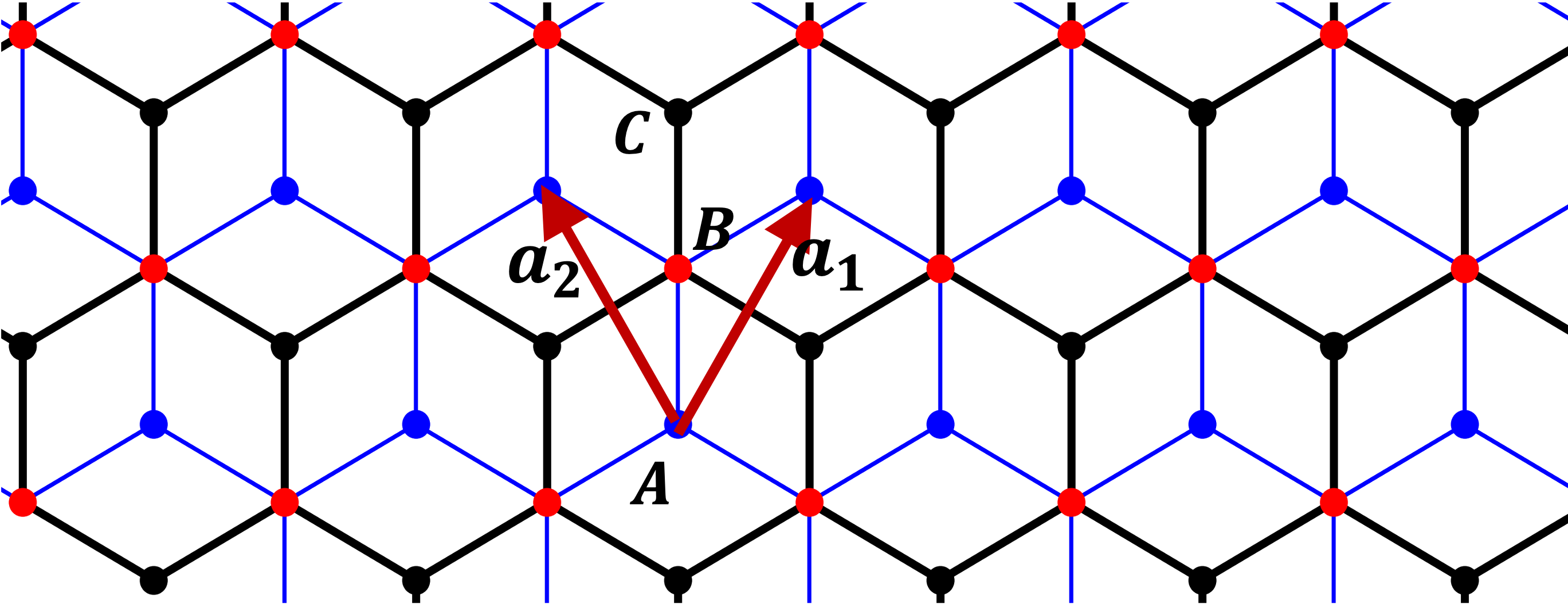
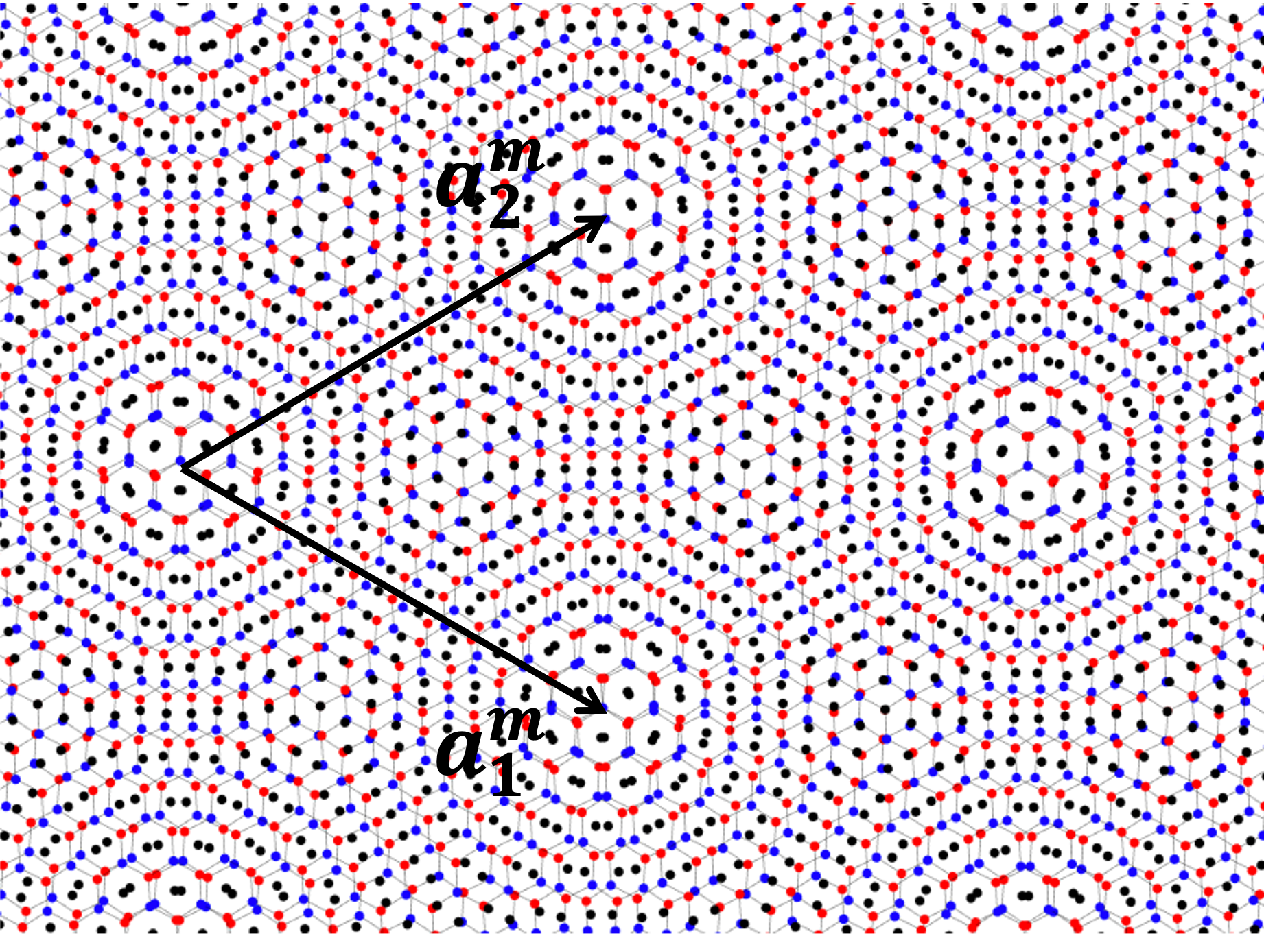
The dice lattice can be viewed as two honeycomb lattices ( and ) sharing the same sublattice site . The lattice base vectors are and and the corresponding reciprocal vectors , and , where is lattice constant, and is the distance between two nearest sites [see Fig. 1(a)]. For simplicity, we consider a spinless lattice model with nearest-neighbor hopping only. Due to this similarity, the TBD has the same moiré structure as TBG [see Fig. 2(a)]. There is a flat band in the lattice spectrum. The low energy behavior near the Dirac point can be captured by , where is the lattice momentum, and is the spin-1 generalization of the Pauli matrix that acts on sublattice space of the order of , , and ,
| (1) |
Since the dice lattice can be realized in the SrTiO3/SrIrO3/SrTiO3 trilayer heterostructure by growing in the (111) direction wang2011 , it is possible to realize the TBD in this material by twisting when growing.
For TBG, Bistritzer and MacDonald proposed a low-energy effective continuum Dirac model of the moiré structure for a small twist angle using Bloch bands near the Dirac points. The effective model consists of two isolated graphene layers and hopping terms between them. With this model they reveal flat Bloch bands in the electric structure at magic twist angles which give rise to a high DOS Bistritzer-MacDonald2011 . Similar to the case of TBG, we follow Ref. Bistritzer-MacDonald2011 to construct a continuum model for the TBD. In principle, for the Bloch-band-based effective theory to be valid, the valley structure should be present. However, the global flat band in the single-layer dice model may negate this validity. This obstacle could be avoided by including the second-nearest-neighbor hopping in the lattice model such that the global flat bands become dispersive and acquire the valley structure. In a recent paper arv2023 Zhou confirmed that the flat-band structure is substantiated in the TBD in the absence of the second-nearest-neighbor hopping. Therefore, we can only consider the nearest-neighbor hopping in the TBD for simplicity. Later we will show that this is the case in the chiral limit of the continuum model, and there are exact flat bands at all angles. In contrast, away from the chiral limit, the results would be less predictive if the second-nearest-neighbor hopping were zero and the valley structure were absent due to the flat bands.
In the TBD, we keep the top layer 1 fixed and rotate the bottom layer 2 by with respect to layer 1. The effective TBD Hamiltonian contains intralayer and interlayer parts. The low-energy intra-Hamiltonian reads
| (2) |
where are the annihilation operators in layers 1 and 2 respectively, and .
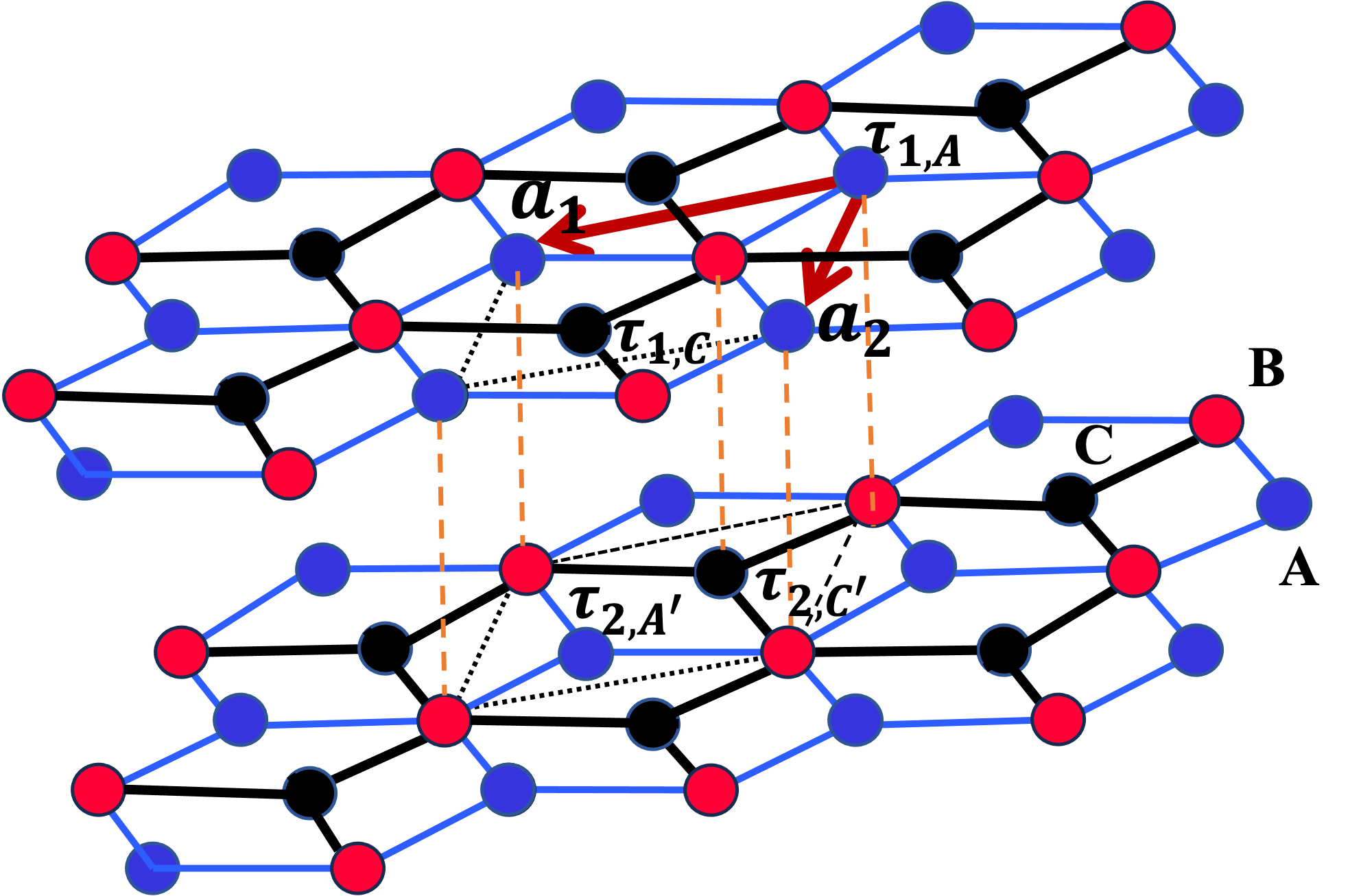
For the interlayer hopping term , we consider nearest-neighbor hopping from layer 1 in the sublattice to the closest sublattice in layer 2 (see Fig. 1). The hopping amplitude depends on the difference between the two sites. We have,
| (3) |
with
| (4) | |||||
where is unit cell area and represent the Dirac point for each layer which satisfies , where is the rotation matrix. Here is a vector connecting the two sites in the unit cell. For the TBD, we consider the stacking (Bernal) configuration coordinates as , , and [see Fig. 1(b)]. To compare the results with TBG, we choose Å, the lattice constant of graphene. Here is the Fourier transformation of the tunneling amplitude which satisfies and decays rapidly if in reciprocal space exceeds the Dirac point Bistritzer-MacDonald2011 . Considering this property we only need to choose three vectors , with , , and the reciprocal lattice vectors, the layer index, and . Substituting these three vectors into the hopping matrix (4), we have
where , , and are the vectors connecting the nearest Dirac points of the two layers in the moiré Brillouin zone [see Fig. 2(b)], and
| (6) |
where with , and . Here we choose meV as in graphene Bistritzer-MacDonald2011 . We choose also , which is the translation vector of the TBD. For later convenience, we also denote the transition amplitude between the two layers by .
II.1 Chiral limit of the TBD
The origin and topological nature of the flat bands can be revealed in the chiral limit. In the Ref. Tarnopolsky2019 , Tarnopolsky . proposed the chirally symmetric continuum model for TBG, which is also known as the chiral limit. In their model they considered a Hamiltonian
with the basis , where and are the layer indices and and correspond to the sublattice. Here is a parameter, is the interlayer potential, and . The chiral symmetry is manifested by the particle-hole symmetry , where acts in the sublattice space. The flat bands in TBG satisfy , which also determines the magic angle, and the flat-band wave function behaves like the one in the quantum Hall effect on a torus Tarnopolsky2019 . Therefore, these flat bands in TBG are topological. Another reason is that the flat bands can be explained as the zeroth Landau level of the Weyl fermion under a pseudomagnetic field which comes from the lattice distortion of the twisting Liu2019Pseudo and the zeroth Landau level of the Weyl fermion is topological.
Inspired by this model, we generalize the chiral limit to the TBD model by substituting from the Pauli matrices that act on the sublattice space to the matrices defined in (1),
| (7) |
with the particle-hole symmetry . The basis is now , where labels the sublattice. Therefore, the generalized chiral symmetry in the TBD corresponds to choosing , and the hopping matrices defined in (6) become
| (8) |
Now we can count the number of flat bands. The usual band counting from TBG at the magic angle is one flat band per valley per spin, with a total number of four, from each of and . In TBD, there are two kinds of flat bands. One is similar to the case of TBG, which comes from and . They produce four flat bands each. The and sublattice indices correspond to the valley indices in TBG. For , and should be satisfied for flat bands. In the limit, this means should be both holomorphic and antiholomorphic, which is a constant if has no singularity. Therefore, does not generate flat bands. The other kind of flat bands originates from the destructive interference of the states on the dice lattice structure. We can construct these wave functions in the limit, to which the model is continuously connected Tarnopolsky2019 , namely, , where , and are constants and are some arbitrary functions of without singularities. The Chern number of these flat bands is zero. This is also confirmed in the pseudo-Landau-level description discussed in Sec. III. From the Landau level point of view, the flat bands corresponding to the zeroth Landau level are topological and the ones from the th Landau level are trivial.
The chiral symmetry of the Hamiltonian (7) can also be confirmed without twisting (see the Appendix). For stacking, finite will break the particle-hole symmetry [see Fig. 3(a)].
II.2 Comparing the band structures of TBG and the TBD
After building the effective model of the TBD, we now can compare the band structures of TBG and the TBD. Similar to Bistritzer and MacDonald’s model for TBG Bistritzer-MacDonald2011 , the Hamiltonian for a layer with the twist angle near the Dirac point can be written as
| (9) |
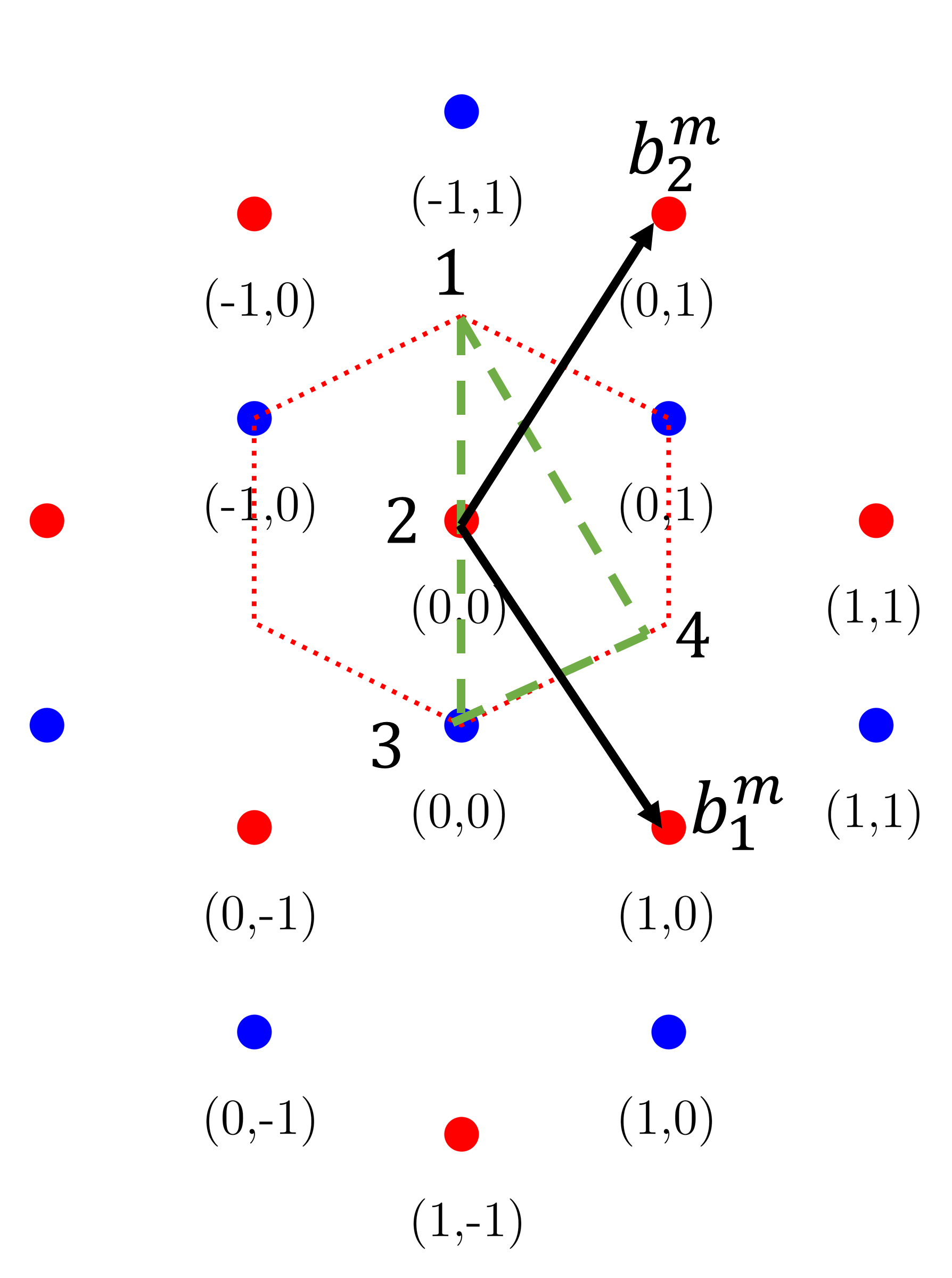
where is the momentum measured from the Dirac point in the moiré Brillouin zone with the unit vectors and where is the size of the moiré unit cell [see Fig. 2(b)]. By using the Bloch bands, we can truncate the TBD model Hamiltonian near the Dirac points in the moiré Brillouin zone. For example, by defining , the simplest case is to truncate to the first moiré Brillouin zone Bistritzer-MacDonald2011 , namely . The truncated Hamiltonian has the form
| (14) |
where is the kinetic part of (9) in layer 1(2). The basis of the above Hamiltonian is four three-component spinors with the momentum near the central Dirac point in layer 1 and , , and in layer 2 [see Fig. 2(b)]. The chiral limit is obtained by replacing the hopping matrices , , and with , , and , respectively.
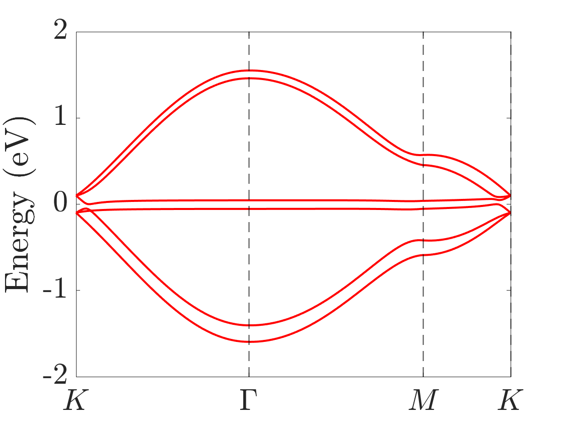
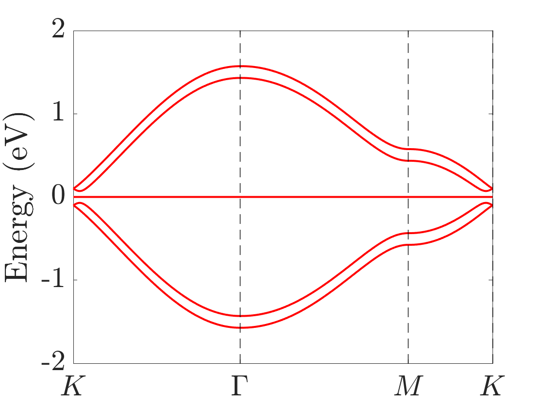
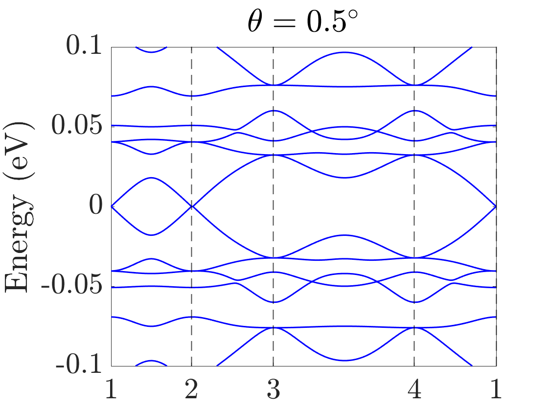
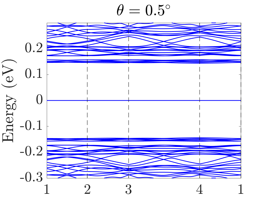
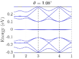
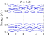
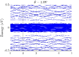
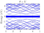
In the numerical calculation, we choose . In TBG, the absolutely flat band at the magic angle can be obtained in the chiral limit, namely, by choosing Tarnopolsky2019 . In the chiral limit of the TBD, highly degenerate flat bands at zero energy also exist. We truncate the Hamiltonian at the order of , and we choose three moiré angles . The final results of the band structures of TBG and the TBD are summarized in Fig.4.
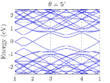
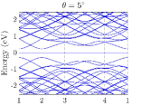
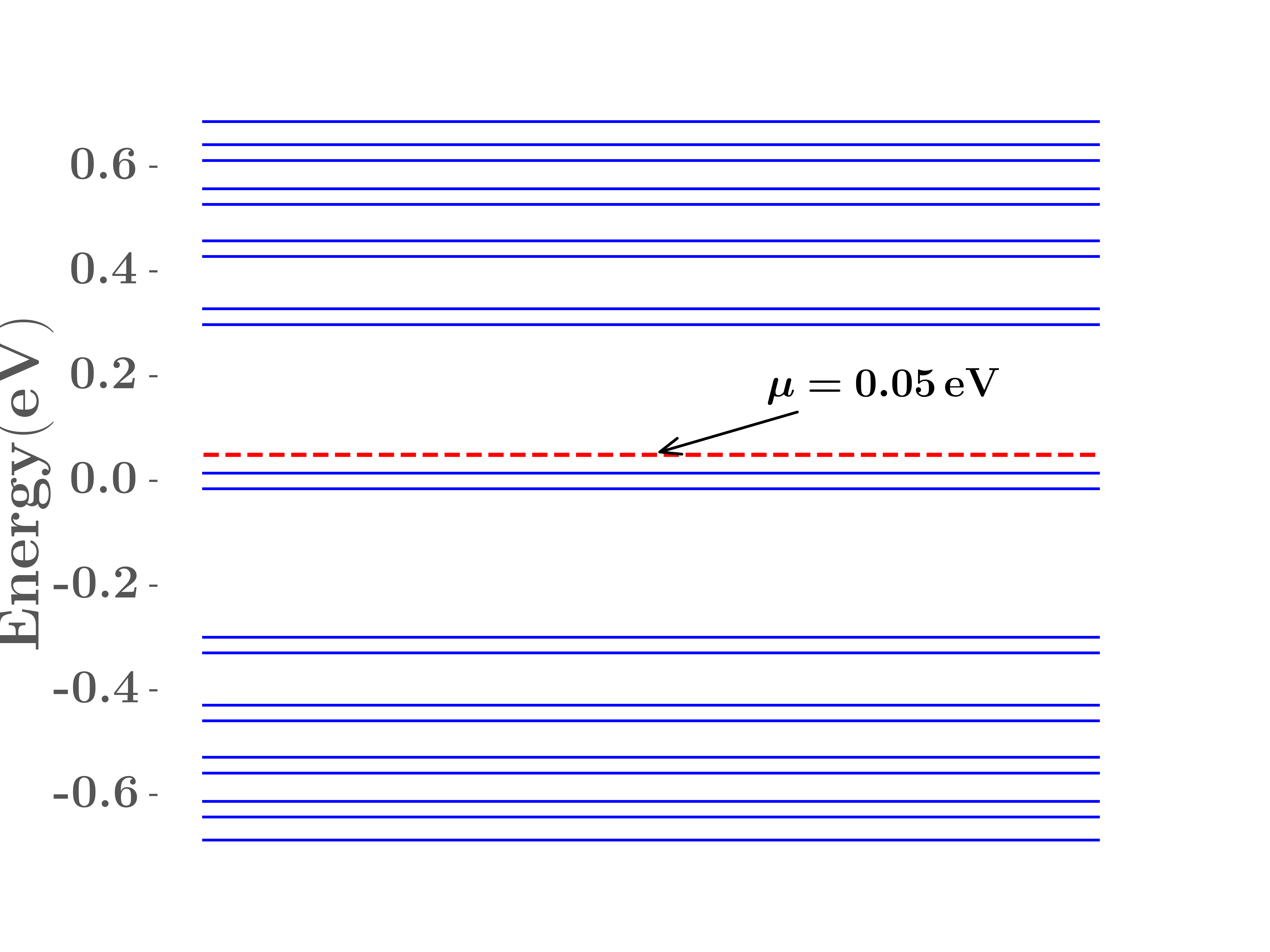
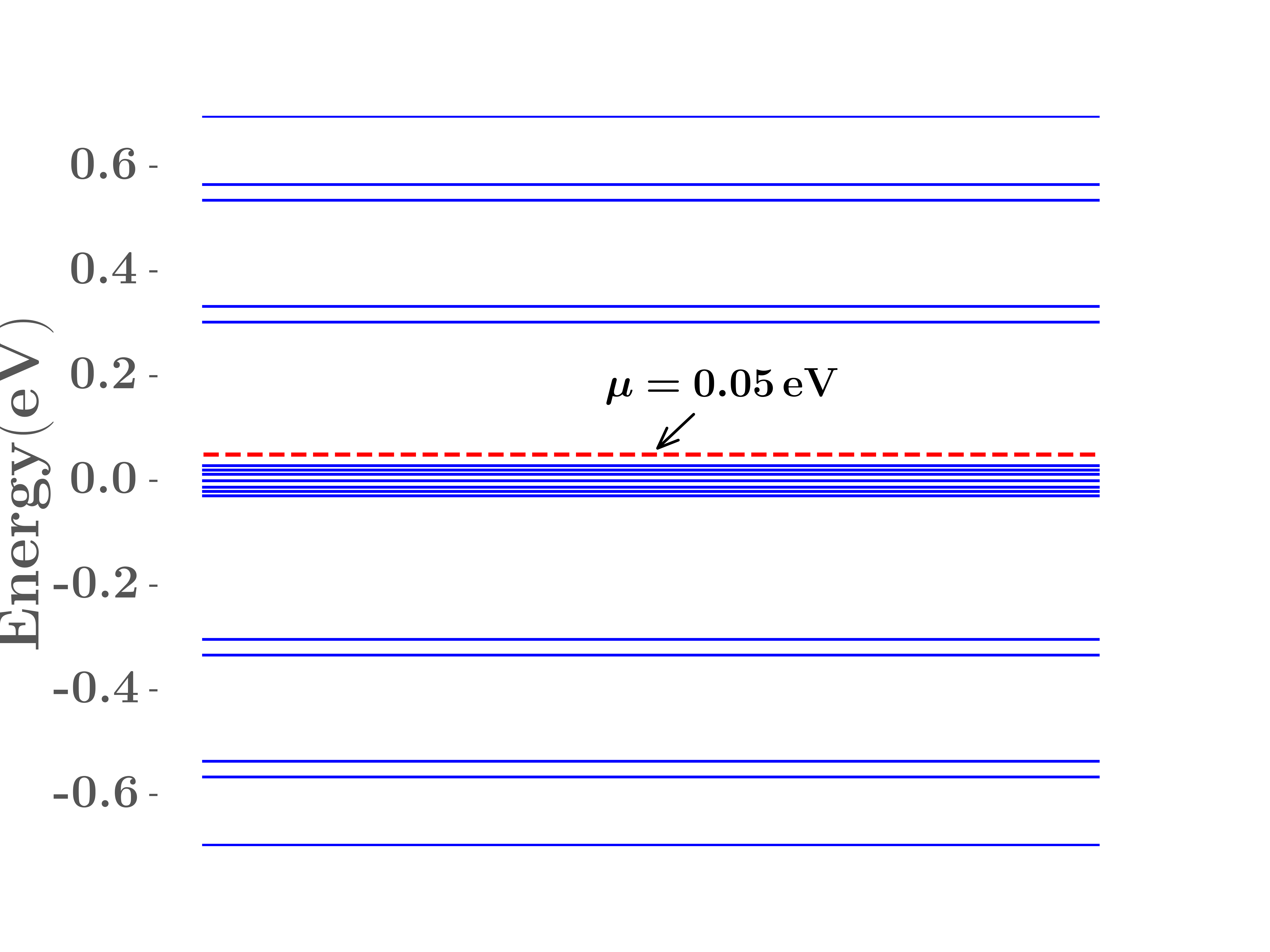
Unlike TBG which only has flat bands near magic angles, the TBD has flat bands at all angles, which is a manifestation of the flat band of the single-layer dice lattice model. These TBD flat bands are highly degenerate in the chiral limit, more than the usual band counting. When chiral symmetry is broken by finite or , the original exactly flat bands in the chiral limit now spread from zero energy and become nearly flat; this behavior is similar to that of Landau levels [see Figs. 4(g) and 5(b)]. Numerically, we find that for small perturbations that break the chiral symmetry, the nearly flat bands are now away from zero energy and the gaps among them and the conduction and valence bands remain [see Figs. 4(g) and 4(h)]. This, however, could be an artifact of the continuum model due to flat bands and the lack of valley structure, which is the limitation of the continuum model away from the chiral limit. To further verify the validity of the continuum model in the flat-band regime, a more controlled calculation, such as a real-space commensurate one, is needed, which is beyond the scope of the present work. Therefore, besides the theoretical analysis in the preceding section, we also numerically confirm that in order to obtain the band structure of exact flat bands at zero energy, namely, the chiral limit, both parameters and must be zero.
Before ending this section, we would like to comment on the degeneracy of the flat bands of the TBD. In general, the degeneracy is lower when away from the magic angle or the chiral limit. In numerical calculations, apply different cutoff parameters for different twist angles, because the size of the unit cell dependent on the twist angle . The smaller the twist angle is, the more Dirac points will be folded in this cutoff. A consequence is that the number of degenerate flat bands decreases as the twist angle increases. Further, the number of flat bands is nearly one-third the number of sites, showing that most of the flat bands originate from the destructive interference of the states on the dice lattice. Our results are consistent with those in Ref. arv2023 .
III The gauge potential and pseudo-Landau-level structure
The chiral limit is an ideal model to study the flat-band structure, while in reality, the chiral limit is violated by finite or arising from different atomic stacking and atomic layer deformation PhysRevB.90.155451 . Fortunately, Liu . showed that Bistritzer and MacDonald’s model for TBG at a small magic angle can be effectively described by pseudo-Landau levels under an gauge potential Liu2019Pseudo . After a gauge transformation on the Bloch functions and expanding the tunneling potential to the linear order of , Liu arrived at the pseudo-Landau-level Hamiltonian for TBG,
| (16) |
where is the gauge potential and the Pauli matrices act on the layer index. In addition, denotes the hopping parameters and denotes . The effective magnetic field T for TBG at Liu2019Pseudo ; San-Jose2012Non-Abelian ; ren2021 . The effective magnetic fields have opposite directions on each layer; therefore, we can define a time-reversal operator , where means complex conjugation. In addition, the time-reversal symmetry is preserved. After a similar treatment, we can also derive the pseudo-Landau-level Hamiltonian for the TBD. By replacing , which acts on the sublattice index of graphene, by , the result is
| (17) |
where denotes hopping parameters and in the TBD, and denotes . In the following numerical calculations, we set eV, and eV.
To discuss the Landau-level structure, we transform the Hamiltonian (17) into the basis that diagonalizes ,
| (18) |
where , , , and . Since is small, we can treat it as a perturbation. Then for the unperturbed Hamiltonian , we define the Landau-level creation operators of the two layers, and , and the nonzero commutators are ,
| (19) |
where . The is block-diagonalized for each layer. We denote by and the eigen wave functions for layers 1 and 2, respectively. The components of and are made of Landau-level wave functions that satisfy , , , and . To be more specific,
| (20) | |||||
| (21) |
where and are the normalizing coefficients and when , .
For layer 1, there are three energies for ,
| (22) |
In the wave function for , the second component , which has a structure similar to that in the flat-band wave function of the dice lattice. For , there are two eigenenergies
| (23) |
which are the first Landau levels, with the wave functions . Here is the topological zeroth Landau level with and .
For layer 2, the derivation for the spectrum and wave function is similar. For , and . The second component of , . For , and . For , , and .
We treat small as a perturbation, which will mix the states between and and lift the degeneracy at zero energy. This is consistent with the results in Sec. II because corresponds to , which breaks the chiral symmetry. This behavior of small is also confirmed numerically [see Fig. 5(b)], which is similar to the band structure in Fig. 4. Here we emphasize a difference between TBG and the TBD. Because of the lack of zero-energy states for in the pseudo-Landau levels of TBG, the effect of is of the third order Liu2019Pseudo , while in the TBD, it is of the first order. Therefore, the optical conductance for finite will behave differently for TBG and the TBD (discussed below). A similarity between TBG and the TBD is that, after the perturbation of , a double degeneracy remains which is related to the symmetry Liu2019Pseudo .
IV Optical conductance
In reality, materials that rotate the polarization plane of linearly polarized light have many applications in various devices, which is usually achieved by magneto-optical effects, the quantum Hall effect, and the Kerr and Faraday rotations by invoking external magnetic fields oc1 ; oc2 ; oc3 ; oc4 ; oc7 , which also limits the applications in small-scale devices. Therefore, searching for materials with intrinsic properties that rotate light is urgent for recent applications. The TBG is such a candidate for advanced optical applications due to the tunable twist angles occ1 ; occ2 . The optical conductivity of the bilayer dice lattice without twisting was studied before suk1 ; suk2 . Here we study the optical conductance of the TBD, which could be another candidate for such applications.
We utilize the Kubo formula in the pseudo-Landau-level basis to calculate the optical conductance of the TBD system PhysRevB.94.125435 ,
| (24) |
where is the magnetic length. Without considering the spin degree of freedom, we can simply set . Here is the Fermi distribution and is the photon energy. Although we use the pseudo-Landau-level description, no external magnetic field is applied. The pseudomagnetic field is induced by the hopping of and , which can also be induced by strain guo2022 .
We take into account the contribution of all Landau levels; however, the remaining double degeneracy of the band structure will cause divergence in conductance. For a doubly degenerate band, we set the divergent part of the Kubo formula (24) as
| (25) |
From the Hamiltonian (19), the current is obtained as .
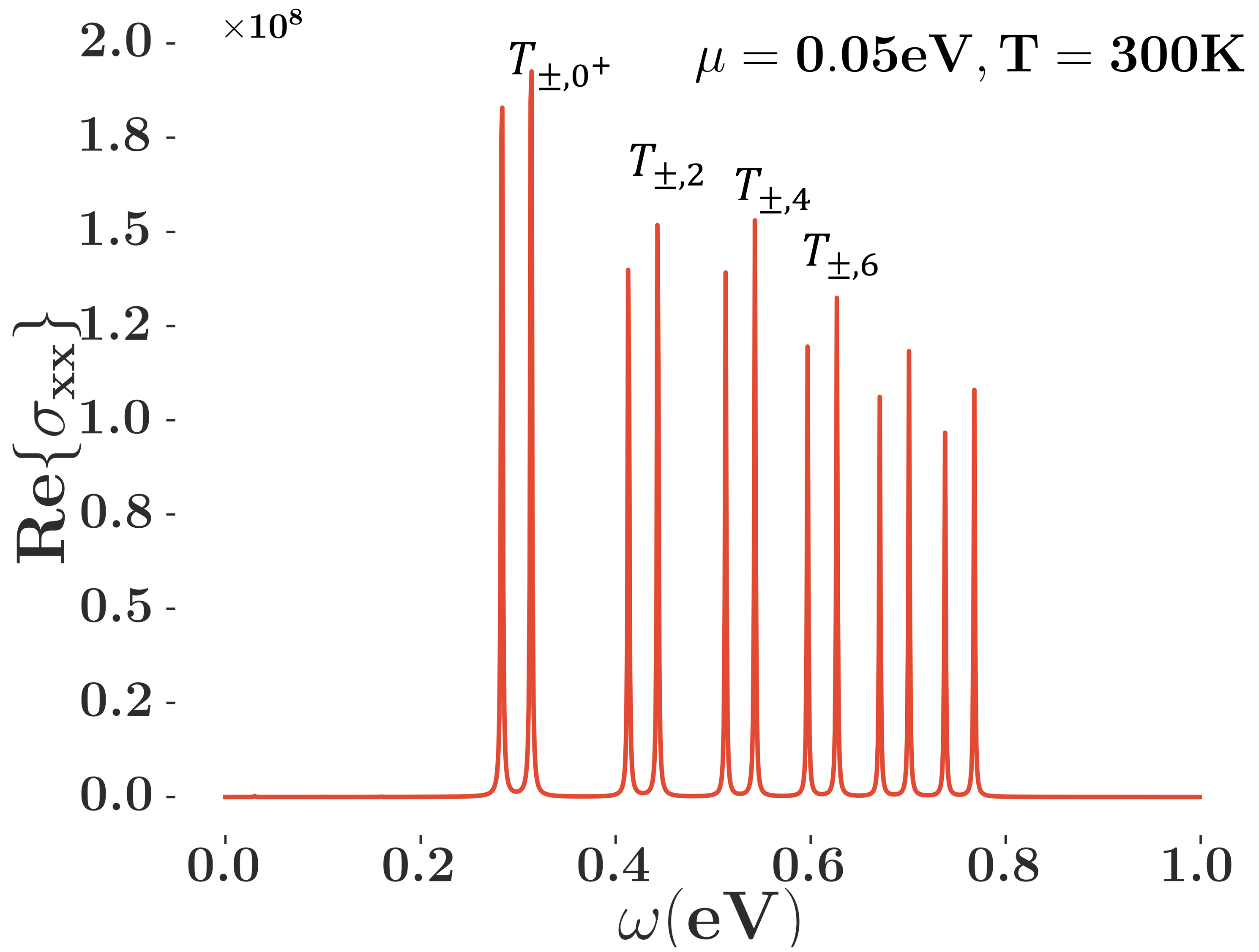
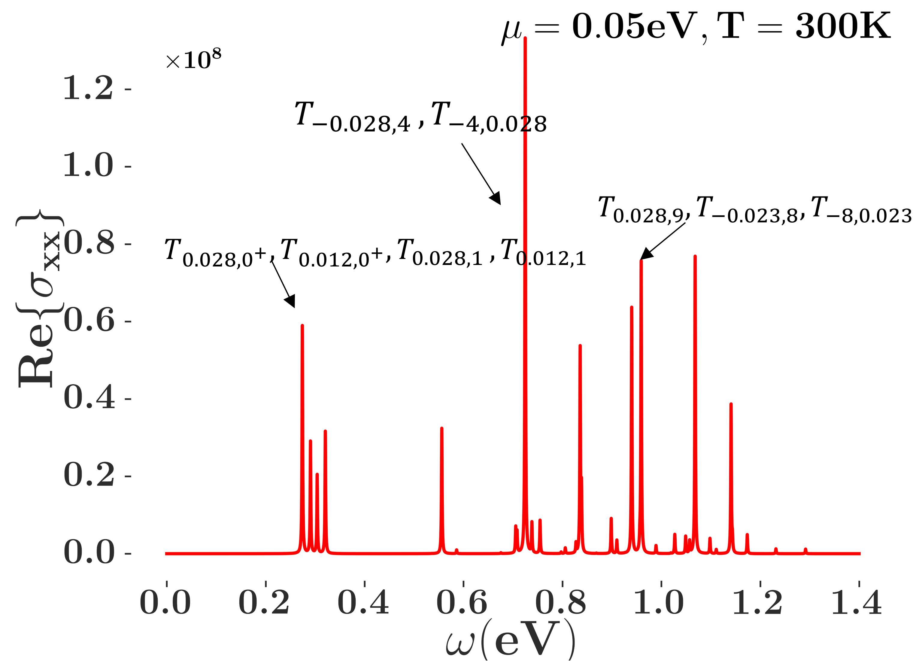
The numerical results for eV and K of the conductance of TBG and the TBD are shown in Figs. 5(c) and 5(d). Since the chemical potential we choose is close to zero, all significant absorption peaks originate from transitions between the near-zero bands and the positive-energy bands, or between the negative-energy bands and the near-zero bands. The double-peak structure of TBG is caused by the splitting of double degeneracy, and the width of the splitting is proportional to .
By comparing the result of TBG with that for the TBD, we see that the double-peak structure of TBG does not exist in the TBD. In the TBD, the peak splits into several small peaks. This reflects that there are many states near zero energy. In Fig. 5(c) the distance between the double peaks is eV, which corresponds to 40 m, while in Fig. 5(d) the typical distance between the split peaks is eV, and the corresponding wave length is about 80 m, which are all in the terahertz range and experimentally detectable. Therefore, this peak-splitting structure provides proof of the experimental prediction showing the existence of the large degeneracy of the flat bands in the TBD.
Although the Landau-level description for TBG fails when the twist angle is away from the magic ones, the Landau-level structure remains in the TBD [see Figs. 4(g) and 4(h)]. Therefore, in the optical conductance at angles other than the magic ones, the peak splitting structure remains in the TBD, whereas the peaks arising from the transitions that form the flat bands disappear in TBG, which is also a key experimental difference between TBG and the TBD.
The transitions between these zero-energy levels are forbidden in the TBD, which means there are no peaks at low frequency near , which is a key difference from the three-dimensional Kane fermion Luo2019 . The reason for this phenomenon is attributed to the structure of the current and wave function in two dimensions, that is, between those near-zero bands, and their contribution to the optical conductance being zero, while in three dimensions, the part will have a nontrivial contribution, and the transition between different Landau levels has a non zero , which causes the peaks near zero frequency Luo2019 .
V Conclusions
In this paper we constructed a lattice model for the TBD. In the chiral limit, it has flat bands at all twisted angles besides the magic ones and the flat bands are broadened when chiral symmetry is broken, which could be confirmed by the peak splitting structure of the optical conductance near the magic angles. Away from the magic angles, the peak splitting remains in the TBD, whereas these peaks disappear in TBG due to the nonexistence of the flat bands. The flat bands in the TBD are composed of zero-Chern-number bands by destructive interference of the states on the dice lattice as well as the topological nontrivial bands by the moiré structure at the magic angles. In this model we have neglected the spin degrees of freedom of electrons. If the spin orbital coupling interaction is added, the bands with zero Chern number may become non-trivial wang2011 . It is possible to realize the TBD in the transition-metal oxide SrTiO3/SrIrO3/SrTiO3 trilayer heterostructure by growing and twisting in the (111) direction. As a semiconductor, due to the high DOS of the flat bands of the TBD, the TBD may have potential applications in temperature-sensitive and photosensitive manipulations. With interactions, the TBD may also be a good candidate as a fractional Chern insulator.
Acknowledgements.
This work was supported by the National Natural Science Foundation of China through Grant No. 12174067.Appendix A Bilayer dice lattice without twisting
In the main text we discussed the effects of finite and on the flat-band structure of the TBD system; here we consider their effects on the band structure in the aligned bilayer case. The Hamiltonian of the stacking bilayer dice lattice reads
| (A1) |
where , , and . The basis of the aligned bilayer dice lattices is . The positions of atoms and in one unit cell are and , and is a lattice constant. Here we have set . The band structures with and were plotted in Fig. 3, where the chiral symmetry is broken for finite .
References
- (1) A. Mielke, Ferromagnetic ground states for the Hubbard model on line graphs, J. Phys. A: Math. Gen. 24, L73 (1991).
- (2) H. Tasaki, Ferromagnetism in the Hubbard models with degenerate single-electron ground states, Phys. Rev. Lett. 69, 1608 (1992).
- (3) S. Zhang, H.-H. Hung, and C. Wu, Proposed realization of itinerant ferromagnetism in optical lattices, Phys. Rev. A 82, 053618 (2010).
- (4) J.-W. Rhim, K. Kim, and B.-J. Yang, Quantum distance and anomalous Landau levels of flat bands, Nature 584, 59 (2020).
- (5) J.-X. Yin, S. S. Zhang, G. Chang, Q. Wang, S. S. Tsirkin, Z. Guguchia, B. Lian, H. Zhou, K. Jiang, I. Belopolski, N. Shumiya, D. Multer, M. Litskevich, T. A. Cochran, H. Lin, Z. Wang, T. Neupert, S. Jia, H. Lei, and M. Z. Hasan, Negative flat band magnetism in a spin–orbit-coupled correlated kagome magnet, Nat. Phys. 15, 443 (2019).
- (6) E. Tang, J.-W. Mei, and X.-G. Wen, High-temperature fractional quantum Hall states, Phys. Rev. Lett. 106, 236802 (2011).
- (7) E. J. Bergholtz, and Z. Liu, Topological flat band models and fractional Chern insulators, International Journal of Modern Physics B 27, 1330017 (2013).
- (8) C. Wu, D. Bergman, L. Balents, and S. Das Sarma, Flat bands and Wigner crystallization in the honeycomb optical lattice, Phys. Rev. Lett. 99, 070401 (2007).
- (9) C. Wu and S. Das Sarma, -orbital counterpart of graphene: Cold atoms in the honeycomb optical lattice, Phys. Rev. B 77, 235107 (2008).
- (10) R. Micnas, J. Ranninger, and S. Robaszkiewicz, Superconductivity in narrow-band systems with local nonretarded attractive interactions, Rev. Mod. Phys. 62, 113 (1990).
- (11) S. Miyahara, S. Kusuta, and N. Furukawa, BCS theory on a flat band lattice, Physica C 460, 1145 (2007).
- (12) H. Aoki, Theoretical possibilities for flat band superconductivity, Journal of Superconductivity and Novel Magnetism 33, 2341 (2020).
- (13) I. Syôzi, Statistics of kagomé lattice, Progress of Theoretical Physics 6, 306 (1951).
- (14) E. H. Lieb, Two theorems on the Hubbard model, Phys. Rev. Lett. 62, 1201 (1989).
- (15) B. Sutherland, Localization of electronic wave functions due to local topology, Phys. Rev. B 34, 5208 (1986).
- (16) Z. Liu, Z.-F. Wang, J.-W. Mei, Y.-S. Wu, and F. Liu, Flat Chern band in a two-dimensional organometallic framework, Phys. Rev. Lett. 110, 106804 (2013).
- (17) Z. Liu, F. Liu, and Y.-S. Wu, Exotic electronic states in the world of flat bands: From theory to material, Chin. Phys. B 23, 077308, (2014).
- (18) P. Sathe, F. Harper, and R. Roy, Compactly supported Wannier functions and strictly local projectors, J. Phys. A: Math. Theor. 54 335302, (2021).
- (19) P. Sathe and R. Roy, Compact Wannier functions in one dimension, arXiv:2302.11608.
- (20) Y.-G. Chen, J.-T. Huang, K. Jiang, J.-P. Hu, Decoding flat bands from compact localized states, arXiv:2212.13526.
- (21) P. Sathe and R. Roy, Topological triviality of flat Hamiltonians, arXiv:2309.06487.
- (22) F. Wang and Y. Ran, Nearly flat band with Chern number on the dice lattice, Phys. Rev. B 84, 241103(R) (2011).
- (23) M. R. Slot, T. S. Gardenier, P. H. Jacobse, G. C.P. van Miert, S. N. Kempkes, S. J.M. Zevenhuizen, C. M. Smith, D. Vanmaekelbergh, and I. Swart, Experimental realization and characterization of an electronic Lieb lattice, Nat. Phys. 13, 672 (2017).
- (24) R. Shen, L. B. Shao, B. Wang, and D. Y. Xing, Single Dirac cone with a flat band touching on line-centered-square optical lattices, Phys. Rev. B 81, 041410(R) (2010).
- (25) D. Guzmán-Silva, C. Mejía-Cortés, M. A. Bandres, M. C. Rechtsman, S. Weimann, S. Nolte, M. Segev, A. Szameit, and R. A. Vicencio, Experimental observation of bulk and edge transport in photonic Lieb lattices, New J. Phys. 16, 063061 (2014).
- (26) S. Mukherjee, , A. Spracklen, D. Choudhury, N. Goldman, P. Ohberg, E. Andersson, and R. R. Thomson, Observation of a localized flat-band state in a photonic Lieb lattice, Phys. Rev. Lett. 114, 245504 (2015).
- (27) R. A. Vicencio, C. Cantillano, L. Morales-Inostroza, B. Real, C. Mejía-Cortés, S. Weimann, A. Szameit, and M. I. Molina, Observation of localized states in Lieb photonic lattices, Phys. Rev. Lett. 114, 245503 (2015).
- (28) S. Taie, H. Ozawa, T. Ichinose, T. Nishio, S. Nakajima, and Y. Takahashi, Coherent driving and freezing of bosonic matter wave in an optical Lieb lattice, Sci. Adv. 1, 1500854 (2015).
- (29) S. Xia, Y. Hu, D. Song, Y. Zong, L. Tang, and Z. Chen, Demonstration of flat-band image transmission in optically induced Lieb photonic lattices, Opt. Lett. 41, 1435 (2016).
- (30) R. Sarkar, A. Bandyopadhyay, and A. Narayan, Non-Hermiticity induced exceptional points and skin effect in the Haldane model on a dice lattice, Phys. Rev. B 107, 035403 (2023).
- (31) X. Luo, F.-Y. Li, and Y. Yu, Anomalous magnetic transport and extra quantum oscillation in semi-metallic photon-like fermion gas, New J. Phys. 20, 083036 (2018).
- (32) M. Orlita, D. M. Basko, M. S. Zholudev, F. Teppe, W. Knap, V. I. Gavrilenko, N. N. Mikhailov, S. A. Dvoretskii, P. Neugebauer, C. Faugeras, A. -L. Barra, G. Martinez, and M. Potemski, Observation of three-dimensional massless Kane fermions in a zinc-blende crystal, Nat. Phys. 10, 233 (2014).
- (33) A. Akrap, M. Hakl, S. Tchoumakov, I. Crassee, J. Kuba, M. O. Goerbig, C. C. Homes, O. Caha, J. Novak, F. Teppe, W. Desrat, S. Koohpayeh, L. Wu, N. P. Armitage, A. Nateprov, E. Arushanov, Q. D. Gibson, R. J. Cava, D. van der Marel, B. A. Piot, C. Faugeras, G. Martinez, M. Potemski, and M. Orlita, Magneto-optical signature of massless Kane electrons in Cd3As2, Phys. Rev. Lett. 117, 136401 (2016).
- (34) X. Luo, Y.-G. Chen, and Y. Yu, Magneto-optical conductance of Kane fermion gas in low frequencies, New J. Phys. 21, 083010 (2019).
- (35) B. Bradlyn, J. Cano, Z. J. Wang, M. G. Vergniory, C. Felser, R. J. Cava, and B. A. Bernevig, Beyond Dirac and Weyl fermions: Unconventional quasiparticles, Science aaf5037 (2016).
- (36) Z. M. Zhu, G. W. Winkler, Q. S. Wu, J. Li, and A. A. Soluyanov, Triple point topological metals, Phys. Rev. X 6, 031003 (2016).
- (37) H. Yang, J. B. Yu, S. S. P. Parkin, C. Felser, C.-X. Liu, and B. H. Yan, Prediction of triple point fermions in simple half-Heusler topological insulators, Phys. Rev. Lett. 119, 136401 (2017).
- (38) K.-H. Ahn, W. E. Pickett, and K.-W. Lee, Coexistence of triple nodal points, nodal links, and unusual flat bands in intermetallic Pd3 (=Pb,Sn), Phys. Rev. B 98, 035130 (2018).
- (39) T. Zhang, Y. Jiang, Z. Song, H. Huang, Y. He, Z. Fang, H. Weng, and C. Fang, Catalogue of topological electronic materials, Nature 566, 475 (2019).
- (40) M. G. Vergniory, L. Elcoro, C. Felser, N. Regnault, B. A. Bernevig, and Z. Wang, A complete catalogue of high-quality topological materials, Nature 566, 480 (2019).
- (41) F. Tang, H. C. Po, A. Vishwanath, and X. Wan, Comprehensive search for topological materials using symmetry indicators, Nature 566, 486 (2019).
- (42) R. Bistritzer and A. H. MacDonald, Moire bands in twisted double-layer graphene, PNAS 108, 12233 (2011).
- (43) E. Y. Andrei, and A. H. MacDonald, Graphene bilayers with a twist, Nature Materials 19, 1265 (2020).
- (44) Y. Cao, V. Fatemi, S. Fang, K. Watanabe, T. Taniguchi, E. Kaxiras, and P. Jarillo-Herrero, Unconventional superconductivity in magic-angle graphene, Nature 556, 43 (2018).
- (45) B. Lian, Z. Wang, and B. A. Bernevig, Twisted bilayer graphene: A phonon-driven superconductor, Phys. Rev. Lett. 122, 257002 (2019).
- (46) K. P. Nuckolls, M. Oh, D. Wong, B. Lian, K. Watanabe, T. Taniguchi, B. A. Bernevig, and A. Yazdani, Strongly correlated Chern insulators in magic-angle twisted bilayer graphene, Nature 588, 610 (2020)
- (47) J. Liu, J. Liu, and X. Dai, Pseudo Landau level representation of twisted bilayer graphene: Band topology and implications on the correlated insulating phase, Phys. Rev. B 99, 155415 (2019).
- (48) G. Tarnopolsky, A.J. Kruchkov, and A. Vishwanath, Origin of magic angles in twisted bilayer graphene, Phys. Rev. Lett. 122, 106405 (2019).
- (49) P. J. Ledwith, G. Tarnopolsky, E. Khalaf, and A. Vishwanath, Fractional Chern insulator states in twisted bilayer graphene: An analytical approach, Phys. Rev. Research 2, 023237 (2020).
- (50) Y. Xie, A. T. Pierce, J. M. Park, D. E. Parker, E. Khalaf, P. Ledwith, Y. Cao, S. H. Lee, S. Chen, P. R. Forrester, K. Watanabe, T. Taniguchi, A. Vishwanath, P. Jarillo-Herrero, and A. Yacoby, Fractional Chern insulators in magic-angle twisted bilayer graphene, Nature 600, 439 (2021).
- (51) J. Cai, E. Anderson, C. Wang, X. Zhang, X. Liu, W. Holtzmann, Y. Zhang, F. Fan, T. Taniguchi, K. Watanabe, Y. Ran, T. Cao, L. Fu, D. Xiao, W. Yao, and X. Xu, Signatures of fractional quantum anomalous Hall states in twisted MoTe2, Nature 622, 63 (2023).
- (52) H. Park, J. Cai, E. Anderson, Y. Zhang, J. Zhu, X. Liu, C. Wang, W. Holtzmann, C. Hu, Z. Liu, T. Taniguchi, K. Watanabe, J. Chu, T. Cao, L. Fu, W. Yao, C. Chang, D. Cobden, D. Xiao, and X. Xu, Observation of fractionally quantized anomalous Hall effect, Nature 622, 74 (2023).
- (53) Y. Zeng, Z. Xia, K. Kang, J. Zhu, P. Knüppel, C. Vaswani, K. Watanabe, T. Taniguchi, K. F. Mak, and J. Shan, Integer and fractional Chern insulators in twisted bilayer MoTe2, arXiv:2305.00973.
- (54) X. Zhou, Y.-C. Hung, B. Wang, and A. Bansil, Generation of isolated flat bands with tunable numbers through Moiré engineering, arXiv: 2310.07647.
- (55) G. Catarina, B. Amorim, E. V. Castro, J. M. V. P. Lopes, and N. Peres, Twisted bilayer graphene: Low-energy physics, electronic and optical Properties, in Handbook of Graphene Set, edited by E. Celasco, A. N. Chaika, T. Stauber, M. Zhang, C. Ozkan, C. Ozkan, U. Ozkan, B. Palys, and S. W. Harun (Wiley, New York, 2019), Chap. 6, pp. 177-231.
- (56) K. Uchida, S. Furuya, J.-I. Iwata, and A. Oshiyama, Atomic corrugation and electron localization due to Moiré patterns in twisted bilayer graphenes, Phys. Rev. B 90, 155451 (2014).
- (57) P. San-Jose, J. Gonzalez, and F. Guinea, Non-Abelian gauge potentials in graphene bilayers, Phys. Rev. Lett. 108, 216802 (2012).
- (58) Y. Ren, Q. Gao, A. H. MacDonald, and Q. Niu, WKB estimate of bilayer graphene’s magic twist angles, Phys. Rev. Lett. 126, 016404 (2021).
- (59) W.-K. Tse and A. H. MacDonald, Magneto-optical Faraday and Kerr effects in topological insulator films and in other layered quantized Hall systems, Phys. Rev. B 84, 205327 (2011).
- (60) I. Crassee, J. Levallois, A. L. Walter, M. Ostler, A. Bostwick, E. Rotenberg, T. Seyller, D. van der Marel, and A. B. Kuzmenko, Giant Faraday rotation in single- and multilayer graphene, Nat. Phys. 7, 48 (2011).
- (61) R. Nandkishore and L. Levitov, Polar Kerr effect and time Reversal symmetry breaking in bilayer graphene, Phys. Rev. Lett. 107, 097402 (2011).
- (62) R. Shimano, G. Yumoto, J. Y. Yoo, R. Matsunaga, S. Tanabe, H. Hibino, T. Morimoto, and H. Aoki, Quantum Faraday and Kerr rotations in graphene, Nat. Commun. 4, 1841 (2013).
- (63) M. L. Solomon, J. Hu, M. Lawrence, A. García-Etxarri, and J. A. Dionne, Enantiospecific optical enhancement of chiral sensing and separation with dielectric metasurfaces, ACS Photonics 6, 43 (2019).
- (64) C.-J. Kim, A. Sáchez-Castillo, Z. Ziegler, Y. Ogawa, C. Noguez, and J. Park, Chiral atomically thin films, Nat. Nanotechnol. 11, 520 (2016).
- (65) S. T. Ho and V. N. Do, Optical activity and transport in twisted bilayer graphene: Spatial dispersion effects, Phys. Rev. B 107, 195141 (2023).
- (66) P. O. Sukhachov, D. O. Oriekhov, and E. V. Gorbar, Stackings and effective models of bilayer dice lattices, Phys. Rev. B 108, 075166 (2023).
- (67) P. O. Sukhachov, D. O. Oriekhov, and E. V. Gorbar, Optical conductivity of bilayer dice lattices, Phys. Rev. B 108, 075167 (2023).
- (68) E. Illes and E. J. Nicol, Magnetic properties of the model: Magneto-optical conductivity and the Hofstadter butterfly, Phys. Rev. B 94, 125435 (2016).
- (69) J. Sun, T. Liu, Y. Du, and H. Guo, Strain-induced pseudo magnetic field in the lattice, Phys. Rev. B 106, 155417 (2022).