MODULI: Unlocking Preference Generalization via Diffusion Models for Offline Multi-Objective Reinforcement Learning

Yifu Yuan, Zhenrui Zheng¹¹footnotemark: 1, Zibin Dong, Jianye Hao
[email protected]
College of Intelligence and Computing, Tianjin University
These authors contribute equally to this work. Work done when ZZ visited Tianjin University.Corresponding authors: Jianye Hao ([email protected])

Abstract

Multi-objective Reinforcement Learning (MORL) seeks to develop policies that simultaneously optimize multiple conflicting objectives, but it requires extensive online interactions. Offline MORL provides a promising solution by training on pre-collected datasets to generalize to any preference upon deployment. However, real-world offline datasets are often conservatively and narrowly distributed, failing to comprehensively cover preferences, leading to the emergence of out-of-distribution (OOD) preference areas. Existing offline MORL algorithms exhibit poor generalization to OOD preferences, resulting in policies that do not align with preferences. Leveraging the excellent expressive and generalization capabilities of diffusion models, we propose MODULI (Multi Objective DiffUsion planner with sLIding guidance), which employs a preference-conditioned diffusion model as a planner to generate trajectories that align with various preferences and derive action for decision-making. To achieve accurate generation, MODULI introduces two return normalization methods under diverse preferences for refining guidance. To further enhance generalization to OOD preferences, MODULI proposes a novel sliding guidance mechanism, which involves training an additional slider adapter to capture the direction of preference changes. Incorporating the slider, it transitions from in-distribution (ID) preferences to generating OOD preferences, patching, and extending the incomplete Pareto front. Extensive experiments on the D4MORL benchmark demonstrate that our algorithm outperforms state-of-the-art Offline MORL baselines, exhibiting excellent generalization to OOD preferences.

1 Introduction

Real-world decision-making tasks, such as robotic control [47, 29], autonomous driving [26], and industrial control [4], often require the optimization of multiple competing objectives simultaneously. It necessitates the trade-offs among different objectives to meet diverse preferences [39]. For instance, in robotic locomotion tasks, users typically focus on the robot’s movement speed and energy consumption [47]. If the user has a high preference for speed, the agent will move quickly regardless of energy consumption; if the user aims to save energy, the agent should adjust to a lower speed. One effective approach is Multi-objective Reinforcement Learning (MORL), which enables agents to interact with vector-rewarded environments and learn policies that satisfy multiple preferences [17, 38, 48]. These methods either construct a set of policies to approximate the Pareto front of optimal solutions [2, 13] or learn a preference-conditioned policy to adapt to any situation [33, 21]. However, exploring and optimizing policies for each preference while alleviating conflicts among objectives, requires extensive online interactions [3], thereby posing practical challenges due to high costs and potential safety risks.

Refer to caption — Figure 1: (Left) Trajectory returns for Hopper-Amateur datasets in D4MORL. We visualize Complete, Shattered, and Narrow datasets for comparison. OOD preference regions are marked by the red circles. (Right) The approximated Pareto fronts learned by MORvS and MODULI on the Shattered dataset.

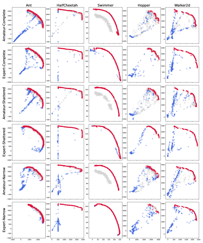
Offline MORL [50] proposes a promising solution that can learn preference-conditioned policies from pre-collected datasets with various preferences, improving data efficiency and minimizing interactions when deploying in high-risk environments. Most Offline MORL approaches focus on extending return-conditioned methods [43, 50] or encouraging consistent preferences through policy regularization [28]. However, real-world offline datasets often come from users with different behavior policies, making it difficult to cover the full range of preferences and leading to missing preference regions, i.e., OOD preferences, resulting in a shattered or narrow data distribution. As shown in fig. 1, we visualize the trajectory returns for Hopper-Amateur dataset. The Complete version of the dataset can comprehensively cover a wide range of preferences. In many cases, suboptimal policies can lead to Shattered or Narrow datasets, resulting in OOD preference regions as marked by the red circles. We then visualize the approximate Pareto front for MORvS baseline [50] and our MODULI in such a shattered dataset. We find that the current Offline MORL baselines exhibit poor generalization performance when learning policies from incomplete datasets. They fail to adapt to OOD preference policies. The approximate Pareto front of MORvS shows significant gaps in the OOD preference areas, indicating that the derived policies and preferences are misaligned. Therefore, we aim to derive a general multi-objective policy that can model a wide range of preference conditions with sufficient expressiveness and strong generalization to OOD preferences. Motivated by the remarkable capabilities of diffusion models in expressiveness and generalization, we propose MODULI (Multi Objective DiffUsion planner with sLIding guidance), transforming the problem of Offline MORL into conditional generative planning. In fig. 1 (right), MODULI demonstrated a better approximation of the Pareto front, achieving returns beyond the dataset. MODULI also patched the missing preference regions and exhibited excellent generalization for the OOD preferences.

MODULI constructs a multi-objective conditional diffusion planning framework that generates long-term trajectories aligned with preference and then executes as a planner. Furthermore, appropriate guiding conditions play a crucial role in the precise generation, which requires the assessment of trajectory quality under different preferences for normalization. We found that simply extending the single-objective normalization method to multi-objective causes issues, as it fails to accurately align preferences with achievable high returns. Therefore, we propose two return normalization methods adapted to multi-objective tasks, which can better measure the quality of trajectories under different preferences and achieve a more refined guidance process. Besides, to enhance generalization to OOD preferences, we introduce a sliding guidance mechanism that involves training an additional slider adapter with the same network structure to independently learn the latent directions of preference changes. During generation, we adjust the slider to actively modify the target distribution, gradually transitioning from ID to specified OOD preferences. This better captures the fine-grained structure of the data distribution and allows for finer control, thereby achieving better OOD generalization. In summary, our contributions include (i) a conditional diffusion planning framework named MODULI, which models general multi-objective policies as conditional generative models, (ii) two preference-return normalization methods suitable for multi-objective preferences to refine guidance, (iii) a novel sliding guidance mechanism in the form of an adapter and, (iv) superior performance in D4MORL, particularly impressive generalization to OOD preferences.

2 Related Work

Offline MORL

Most MORL research primarily focuses on online settings, aiming to train a general preference-conditioned policy [21, 32] or a set of single-objective policies [35, 47] that can generalize to arbitrary preferences. This paper considers an offline MORL setting that learns policy from static datasets without online interactions. PEDI [45] combines the dual gradient ascent with pessimism to multi-objective tabular MDPs. MO-SPIBB [43] achieves safe policy improvement within a predefined set of policies under constraints. These methods often require a priori knowledge about target preferences. PEDA [50] first develops D4MORL benchmarks for scalable Offline MORL with a general preference for high-dimensional MDPs with continuous states and actions. It also attempts to solve the Offline MORL via supervised learning, expanding return-conditioned sequential modeling to the MORL, such as MORvS [12], and MODT [6]. [28] integrates policy-regularized into the MORL methods to alleviate the preference-inconsistent demonstration problem. This paper investigates the generalization problem of OOD preference, aiming to achieve better generalization through more expressive diffusion planners and the guidance of transition directions by a slider adapter.

Diffusion Models for Decision Making

Diffusion models (DMs) [19, 42] have become a mainstream class of generative models. Their remarkable capabilities in complex distribution modeling demonstrate outstanding performance across various domains [24, 40], inspiring research to apply DMs to decision-making tasks [7, 49, 46]. Applying DMs for decision-making tasks can mainly be divided into three categories [51]: generating long horizon trajectories like planner [22, 9, 1], serving as more expressive multimodal polices [44, 16] and performing as the synthesizers for data augmentation [31]. Diffusion models exhibit excellent generalization and distribution matching abilities [23, 27], and this property has also been applied to various types of decision-making tasks such as multi-task RL [18], meta RL [36] and aligning human feedback [10]. In this paper, we further utilize sliding guidance to better stimulate the generalization capability of DMs, rather than merely fitting the distribution by data memorization [15].

3 Preliminaries

Multi-objective RL

The MORL problem can be formulated as a multi-objective Markov decision process (MOMDP) [5]. A MOMDP with $n$ objectives can be represented by a tuple $\langle\mathcal{S},\mathcal{A},\mathcal{P},\mathcal{R},\Omega,\gamma\rangle$ , where $\mathcal{S}$ and $\mathcal{A}$ demote the state and action spaces, $\mathcal{P}$ is the transition function, $\mathcal{R}:\mathcal{S}\times\mathcal{A}\rightarrow\mathbb{R}^{n}$ is the reward function that outputs $n$ -dim vector rewards $\bm{r}=\mathcal{R}(\bm{s},\bm{a})$ , $\Omega$ is the preference space containing vector preferences $\bm{\omega}$ , and $\gamma$ is a discount factor. The policy $\pi$ is evaluated for $m$ distinct preferences $\{\bm{\omega}_{p}\}_{p=1}^{m}$ , resulting policy set be represented as $\{\pi_{p}\}_{p=1}^{m}$ , where $\pi_{p}=\pi(\bm{a}|\bm{s},\bm{\omega}_{p})$ , and $\bm{G}^{\pi_{p}}=\mathbb{E}_{\bm{a}_{t}\sim\pi_{p}}\left[\sum_{t}\gamma^{t}\mathcal{R}(\bm{s}_{t},\bm{a}_{t})\right]$ is the corresponding unweighted expected return. We say the solution $\bm{G}^{\pi_{p}}$ is dominated by $\bm{G}^{\pi_{q}}$ when $G_{i}^{\pi_{p}}<G_{i}^{\pi_{q}}$ for $\forall i\in[1,2,\cdots,n]$ . The Pareto front $P$ of the policy $\pi$ contains all its solutions that are not dominated. In MORL, we aim to define a policy such that its empirical Pareto front is a good approximation of the true one. While not knowing the true front, we can define a set of metrics for relative comparisons among algorithms, e.g., hypervolume, sparsity, and return deviation, to which we give a further explanation in Section 5.

Denoising Diffusion Implicit Models (DDIM)

Assume the random variable $\bm{x}^{0}\in\mathbb{R}^{D}$ follows an unknown distribution $q_{0}(\bm{x}^{0})$ . DMs define a forward process $\{\bm{x}^{t}\}_{t\in[0,T]}$ ¹¹1To ensure clarity, we establish the convention that the superscript $t$ denotes the diffusion timestep, while the subscript $t$ represents the decision-making timestep. by the noise schedule $\{\alpha_{t},\sigma_{t}\}_{t\in[0,T]}$ , s.t., $\forall t\in[0,T]$ :

{\rm d}\bm{x}^{t}=f(t)\bm{x}^{t}{\rm d}t+g(t){\rm d}\bm{w}^{t},~{}\bm{x}^{0}\sim q_{0}(\bm{x}^{0}),

(1)

where $\bm{w}^{t}\in\mathbb{R}^{D}$ is the standard Wiener process, and $f(t)=\frac{{\rm d}\log\alpha_{t}}{{\rm d}t}$ , $g^{2}(t)=\frac{{\rm d}\sigma^{2}_{t}}{{\rm d}t}-2\sigma^{2}_{t}\frac{{\rm d}\log\alpha_{t}}{{\rm d}t}$ . The SDE forward process in Equation 1 has an probability flow ODE (PF-ODE) reverse process from time $T$ to $0$ [42]:

\frac{{\rm d}\bm{x}^{t}}{{\rm d}t}=f(t)\bm{x}^{t}-\frac{1}{2}g^{2}(t)\nabla_{\bm{x}}\log q_{t}(\bm{x}^{t}),~{}\bm{x}^{T}\sim q_{T}(\bm{x}^{T}),

(2)

where the score function $\nabla_{\bm{x}}\log q_{t}(\bm{x}^{t})$ is the only unknown term. Once we have estimated it, we can sample from $q_{0}(\bm{x}^{0})$ by solving Equation 2. In practice, we train a neural network $\bm{\epsilon}_{\theta}(\bm{x}^{t},t)$ to estimate the scaled score function $-\sigma_{t}\nabla_{\bm{x}}\log q_{t}(\bm{x}^{t})$ by minimizing the score matching loss:

\mathcal{L}_{\text{SM}}(\theta)=\mathbb{E}_{t\sim U(0,T),\bm{x}^{0}\sim q_{0}(\bm{x}^{0}),\epsilon\sim\mathcal{N}(\bm{0},\bm{I})}\left[\|\bm{\epsilon}_{\theta}(\bm{x}^{t},t)-\bm{\epsilon}\|^{2}_{2}\right].

(3)

Since $\bm{\epsilon}_{\theta}(\bm{x}^{t},t)$ can be considered as a predicted Gaussian noise added to $\bm{x}^{t}$ , it is called the noise prediction model. With a well-train noise prediction model, DDIM [41] discretizes the PF-ODE to the first order for solving, i.e., for each sampling step:

\bm{x}^{t}=\alpha_{t}\left(\frac{\bm{x}^{s}-\sigma_{t}\bm{\epsilon}_{\theta}(\bm{x}^{s},s)}{\alpha_{s}}\right)+\sigma_{s}\bm{\epsilon}_{\theta}(\bm{x}^{s},s)

(4)

holds for any $0\leq t<s\leq T$ . To enable the diffusion model to generate trajectories based on specified properties, Classifier Guidance (CG) [8] and Classifier-free Guidance (CFG) [20] are the two main techniques. We use CFG due to its stable and easy-to-train properties. CFG directly uses a conditional noise predictor to guide the solver:

\tilde{\bm{\epsilon}_{\theta}}(\bm{x}^{t},t,\bm{c}):=w\cdot\bm{\epsilon}_{\theta}(\bm{x}^{t},t,\bm{c})+(1-w)\cdot\bm{\epsilon}_{\theta}(\bm{x}^{t},t),

(5)

where $w$ is used to control the guidance strength.

4 Methodology

To address the challenges of expressiveness and generalization in Offline MORL, we propose a novel Offline MORL framework called MODULI. This framework utilizes conditional diffusion models for preference-oriented trajectory generation and establishes a general policy suitable for a wide range of preferences while also generalizing to OOD preferences. MODULI first defines a conditional generation and planning framework and corresponding preference-return normalization methods. Moreover, to enhance generalization capability, we design a sliding guidance mechanism, where a slider adapter actively adjusts the data distribution from known ID to specific OOD preference, thereby avoiding simple memorization.

4.1 Offline MORL as Conditional Generative Planning

We derive policies on the Offline MORL dataset $\mathcal{D}$ with trajectories $\tau=(\bm{\omega},\bm{s}_{0},\bm{a}_{0},\bm{r}_{0},\cdots,\bm{s}_{T-1},\bm{a}_{T-1},\bm{r}_{T-1})$ to respond to arbitrary target preferences $\bm{\omega}\in\Omega$ during the deployment phase. Previous Offline MORL [50] algorithms generally face poor expressiveness, unable to adapt to a wide range of preferences through a general preference-conditioned policy, resulting in sub-optimal approximate Pareto front. Inspired by the excellent expressiveness of diffusion models in decision making [1, 10], MODULI introduces diffusion models to model the policy. We define the sequential decision-making problem as a conditional generative objective $\max_{\theta}\mathbb{E}_{\tau\sim\mathcal{D}}\left[\log p_{\theta}\left(\bm{x}^{0}(\tau)\mid\bm{y}(\tau)\right)\right]$ , where $\theta$ is the trainable parameter. The diffusion planning in MORL aims to generate sequential states $\bm{x}^{0}(\tau)=[\bm{s}_{0},\cdots,\bm{s}_{H-1}]$ with horizon $H$ to satisfy the denoising conditions $\bm{y}=[\bm{\omega},\bm{g}]$ , where $\bm{\omega}$ is a specific preference. Similar to [50], $\bm{g}_{t}$ is defined as the vector-valued Returns-to-Go (RTG) for a single step, i.e. $\bm{g}_{t}=\sum_{t}^{T}\mathcal{R}(\bm{s}_{t},\bm{a}_{t})$ . The trajectory RTG $\bm{g}$ is the average of the RTGs at each step.

Training

Next, we can sample batches of $\bm{x}^{0}(\tau)$ and $\bm{y}$ from the dataset and update $p_{\theta}$ as the modified score matching objective in eq. 3:

\mathcal{L}(\theta)=\mathbb{E}_{(\bm{x}^{0},\bm{\omega},\bm{g})\sim\mathcal{D},t\sim U(0,T),\epsilon\sim\mathcal{N}(\bm{0},\bm{I})}\left[\|\bm{\epsilon}_{\theta}(\bm{x}^{t},t,\bm{\omega},\bm{g})-\bm{\epsilon}\|^{2}_{2}\right].

(6)

MODULI uses the CFG guidance for conditional generation. During training, MODULI learns both a conditioned noise predictor $\epsilon_{\theta}(\bm{x}^{t},t,\bm{\omega},\bm{g})$ and an unconditioned one $\epsilon_{\theta}(\bm{x}^{t},t,\varnothing)$ . We adopt a masking mechanism for training, with a probability of $0<p<1$ to zero out the condition of a trajectory, equivalent to an unconditional case. MODULI also employs a loss-weight trick, setting a higher weight for the next state $\bm{s}_{1}$ of the trajectory $\bm{x}^{0}(\tau)$ to encourage more focus on it, closely related to action execution.

4.2 Refining Guidance via Preference-Return Normalization Methods

Global Normalization

To perform generation under different scales and physical quantities of objectives, it is essential to establish appropriate guiding conditions, making return normalization a critical component. We first consider directly extending the single-objective normalization scheme to the multi-objective case, named Global Normalization. We normalize each objective’s RTG using min-max style, scaling them to a unified range. Specifically, we calculate the global maximum RTG $\bm{g}^{\text{max}}=\left[g_{1}^{\text{max}},\cdots,g_{n}^{\text{max}}\right]$ for each objective in the offline dataset. The same applies to the minimum RTG $\bm{g}^{\text{min}}$ . The conditioned RTG $\bm{g}$ are first normalized to $(\bm{g}-\bm{g}^{\text{min}})/(\bm{g}^{\text{max}}-\bm{g}^{\text{min}})\in[0,1]^{n}$ , then concatenated with the preference $\bm{\omega}$ as inputs. During deployment, we aim to generate $\bm{x}(\tau)$ to align the given preference $\bm{\omega}_{\text{target}}$ and maximized scalarized return using the highest RTG condition $\bm{g}=\bm{1}^{n}$ . Note that we compute the global extremum values based on the offline dataset with different preferences, which are not necessarily the reachable min/max value for each objective. Also, some objectives are inherently conflicting and can’t maximized at the same time. As a result, direct guidance using the target conditions of $\bm{y}=[\bm{\omega}_{\text{target}},\bm{1}^{n}]$ may be unachievable for some preferences, leading to a performance drop. To address these issues, we match preferences with vector returns and then propose two novel normalization methods that adapt to multi-objective scenarios to achieve preference-related return normalization, providing more refined guidance: Preference Predicted Normalization and Neighborhood Preference Normalization:

Preference Predicted Normalization

To avoid the issue in Global Normalization, we hope to obtain corresponding RTG conditioned on the given preference. The dataset contains a discrete preference space and it is not possible to directly obtain the maximum RTG for each preference. Therefore, we propose Preference Predicted Normalization training a generalized return predictor additionally $\bm{g}^{\text{max}}(\bm{\omega})=\bm{R}_{\psi}(\bm{\omega})$ to capture the maximum expected return achievable for a given preference $\bm{\omega}$ . Specifically, we first identify all undominated solution trajectories $\tau_{P}\in D_{P}$ , where $D_{P}\subseteq D$ and $P$ demotes Pareto front. Then the generalized return predictor is trained by minimizing the return prediction error conditioned on the preference $\bm{\omega}$ :

\mathcal{L}(\psi)=-\mathbb{E}_{(\bm{\omega},\hat{\bm{g}})\sim D_{P}}\left[\|\bm{R}_{\psi}(\bm{\omega})-\hat{\bm{g}}\|^{2}_{2}\right],

(7)

Then we calculate normalized RTG for each trajectory $\tau$ with preference $\bm{\omega}$ as $\bm{g}_{\tau}/\bm{g}_{\text{max}}(\bm{\omega})\in[0,1]^{n}$ . With RTG prediction, we can follow closer to the training distribution, guiding the generation by specifying different maximum vector returns for each preference.

Neighborhood Preference Normalization

We train $\bm{R}_{\psi}(\bm{\omega})$ using only non-dominated solutions to predict the expected maximum RTG. If the quality of the behavior policy in the dataset is relatively low, the non-dominated solutions in the dataset are sparse, which introduces prediction errors that result in inaccurate normalization. Therefore we propose a simpler, learning-free method named Neighborhood Preference Normalization. In a linear continuous preference space, similar preferences typically lead to similar behaviors. Therefore, we can use a neighborhood set of trajectories to obtain extremum values, avoiding inaccurate prediction. For a trajectory $\tau$ and its corresponding preference $\bm{\omega}_{\tau}$ , we define $\epsilon\text{-neighborhood}$ :

\mathcal{B}_{\epsilon}(\tau)=\left\{\tau^{\prime}\mid\|\bm{\omega}_{\tau^{\prime}}-\bm{\omega}_{\tau}\|\leq\epsilon\right\}

(8)

Therefore, we can use the maximum expected return within the neighborhood trajectories to approximate the maximum expected return, normalized as follows:

	$\displaystyle\bm{g}_{\tau}$	$\displaystyle=\frac{\bm{g}_{\tau}-\min\left(\bm{g}_{\mathcal{B}_{\epsilon}(\tau)}\right)}{\max\left(\bm{g}_{\mathcal{B}_{\epsilon}(\tau)}\right)-\min\left(\bm{g}_{\mathcal{B}_{\epsilon}(\tau)}\right)}\in[0,1],$		(9)
	$\displaystyle\bm{g}_{\mathcal{B}_{\epsilon}(\tau)}$	$\displaystyle=\left\{\bm{g}_{\tau^{\prime}}\mid\tau^{\prime}\in\mathcal{B}_{\epsilon}(\tau)\right\}.$		(10)

Overall, we empirically find that this method can achieve consistently good performance across datasets of various qualities. We leave the comparison of the three normalization methods in the section 5.3 and appendix C.

Action Extraction

Now, MODULI can accurately generate desired trajectories with arbitrary preference and RTG in the CFG manner according to eq. 5. Then, we train an additional inverse dynamics model $a_{t}=h(s_{t},s_{t+1})$ to extract the action $a_{t}$ to be executed from generated $\bm{x}$ . It is worth noting that we fixed the initial state as $\bm{x}^{k}[0]=\bm{x}^{0}[0]$ to enhance the consistency of the generated results.

4.3 Enhancing OOD Preference Generalization with Sliding Guidance

After using diffusion models with appropriate normalization, MODULI can exhibit remarkable expressive capabilities, fully covering the ID distribution in the dataset. However, when faced with OOD preferences, it tends to conservatively generate the trajectory closest to the ID preferences. This may indicate that the diffusion model has overfitted the dataset rather than learning the underlying distribution. To enhance generalization to OOD preferences, inspired by [14] and [11], we propose a novel sliding guidance mechanism. After training the diffusion models $p_{\theta}$ , We additionally trained a plug-and-play slider adapter with the same network structure of diffusion models, which learns the latent direction of preference changes. This enables controlled continuous concept during generation, actively adjusting the target distribution, thus avoiding simple memorization. We define the adapter as $p_{\theta^{*}}$ . When conditioned on $c$ , this method boosts the possibility of attribute $c_{+}$ while reduces the possibility of attribute $c_{-}$ according to original model $p_{\theta}$ :

p_{\theta}\left(\bm{x}^{0}(\tau)\mid c\right)\leftarrow p_{\theta}\left(\bm{x}^{0}(\tau)\mid c\right)\left(\frac{p_{\theta}^{*}\left(c_{+}\mid\bm{x}^{0}(\tau)\right)}{p_{\theta}^{*}\left(c_{-}\mid\bm{x}^{0}(\tau)\right)}\right)^{\eta}

(11)

Based on eq. 11, we can derive a direct fine-tuning scheme that is equivalent to modifying the noise prediction model. The derivation process is provided in the appendix D:

\epsilon_{\theta^{*}}\left(\bm{x}^{t},c,t\right)\leftarrow\epsilon_{\theta}^{*}\left(\bm{x}^{t},c,t\right)+\eta\left(\epsilon_{\theta}\left(\bm{x}^{t},c_{+},t\right)-\epsilon_{\theta}\left(\bm{x}^{t},c_{-},t\right)\right)

(12)

The score function proposed in eq. 12 justifies the distribution of the condition $c$ by converging towards the positive direction $c_{+}$ while diverging from the negative direction $c_{-}$ . Therefore, we can let the $\theta^{*}$ model capture the direction of preference changes, that is, we hope that the denoising process of $\epsilon_{\theta}^{*}(x^{t},c,t)$ at each step meets the unit length shift, i.e. $\epsilon_{\theta^{*}}(x^{t},c,t)=\frac{[c_{\theta}(x^{t},c_{+},t)-c_{\theta}(x^{t},c_{-},t)]}{c_{+}-c_{-}}$ . In MORL tasks, the condition $c$ is $\omega$ , and $c^{+}$ and $c^{-}$ are the changes in preference $\Delta\omega$ in the positive and negative directions, respectively. We minimize the loss $\mathcal{L}(\theta^{*})$ to train the adapter:

\mathcal{L}(\theta^{*})=\mathbb{E}_{(\bm{\omega},\bm{\Delta\omega})\sim D}\left[\left\|\epsilon_{\theta^{*}}(\bm{x}^{t},\bm{\omega},t)-\frac{[\epsilon_{\theta}(\bm{x}^{t},\bm{\omega}+\Delta{\bm{\omega}},t)-\epsilon_{\theta}(\bm{x}^{t},\bm{\omega}-\Delta\bm{\omega},t)]}{2\Delta\bm{\omega}}\right\|_{2}^{2}\right]

(13)

During deployment, when we encounter OOD preferences $\bm{\omega}_{\text{OOD}}$ , we can first transition from the nearest ID preference $\bm{\omega}_{\text{ID}}$ . Then, we calculate $\Delta\bm{\omega}=\bm{\omega}_{\text{OOD}}-\bm{\omega}_{\text{ID}}$ , and at each denoising step, simultaneously apply the diffusion model and adapter as $\epsilon_{\theta}+\Delta\bm{\omega}\epsilon_{\theta^{*}}$ , so that the trajectory distribution gradually shifts from ID preferences to OOD preferences to achieve better generalization. We provide the pseudo code for the entire training and deployment process in appendix E.

5 Experiments

We conduct experiments on various Offline MORL tasks to study the following research questions (RQs): Expressiveness (RQ1) How does MODULI perform on Complete dataset compared to other baselines? Generalizability (RQ2) Does MODULI exhibit leading generalization performance in the OOD preference of Shattered or Narrow datasets? Normalization (RQ3) How do different normalization methods affect performance? All experimental details of MODULI are in appendix B.

Table 1: HV and SP performance on Complete datasets. (B: behavioral policy). The best scores are emphasized in bold. Please refer to appendix F for the full results of the Complete datasets at the expert and amateur levels.

	Env	Metrics	B	MODT(P)	MORvS(P)	BC(P)	CQL(P)	MODULI
Expert	Ant	HV ( $\times 10^{6}$ ) $\uparrow$	6.32	6.21±.01	6.36±.02	4.88±.17	5.76±.10	6.39±.02
	Ant	SP ( $\times 10^{4}$ ) $\downarrow$	-	8.26±2.22	0.87±.19	46.20±16.40	0.58±.10	0.79±.12
	HalfCheetah	HV ( $\times 10^{6}$ ) $\uparrow$	5.79	5.73±.00	5.78±.00	5.54±.05	5.63±.04	5.79±.00
	HalfCheetah	SP ( $\times 10^{4}$ ) $\downarrow$	-	1.24±.23	0.67±.05	1.78±.39	0.10±.00	0.07±.00
	Hopper	HV ( $\times 10^{7}$ ) $\uparrow$	2.09	2.00±.02	2.02±.02	1.23±.10	0.33±.39	2.09±.01
	Hopper	SP ( $\times 10^{5}$ ) $\downarrow$	-	16.30±10.60	3.03±.36	52.50±4.88	2.84±2.46	0.09±.01
	Swimmer	HV ( $\times 10^{4}$ ) $\uparrow$	3.25	3.15±.02	3.24±.00	3.21±.00	3.22±.08	3.24±.00
	Swimmer	SP ( $\times 10^{0}$ ) $\downarrow$	-	15.00±7.49	4.39±.07	4.50±.39	13.60±5.31	4.43±.38
	Walker2d	HV ( $\times 10^{6}$ ) $\uparrow$	5.21	4.89±.05	5.14±.01	3.74±.11	3.21±.32	5.20±.00
	Walker2d	SP ( $\times 10^{4}$ ) $\downarrow$	-	0.99±.44	3.22±.73	75.60±52.30	6.23±10.70	0.11±.01
	Hopper-3obj	HV ( $\times 10^{10}$ ) $\uparrow$	3.73	3.38±.05	3.42±.10	2.29±.07	0.78±.24	3.57±.02
	Hopper-3obj	SP ( $\times 10^{5}$ ) $\downarrow$	-	1.40±.44	2.72±1.93	0.72±.09	2.60±3.14	0.07±.00

Datasets and Baselines

We evaluate MODULI on D4MORL [50], an Offline MORL benchmark consisting of offline trajectories from 6 multi-objective MuJoCo environments. D4MORL contains two types of quality datasets: Expert dataset collected by pre-trained expert behavioral policies, and Amateur dataset collected by perturbed behavioral policies. We named the original dataset of D4MORL as the Complete dataset, which is used to verify expressiveness ability to handle multi-objective tasks. Additionally, to evaluate the algorithm’s generalization ability to out-of-distribution (OOD) preferences, similar to fig. 1, we collected two types of preference-deficient datasets namely Shattered and Narrow. We compare MODULI with various strong offline MORL baselines: BC(P), MORvS(P) [12], MODT(P) [6] and MOCQL(P) [25]. These algorithms are modified variants of their single-objective counterparts and well-studied in PEDA [50]. MODT(P) and MORvS(P) view MORL as a preference-conditioned sequence modeling problem with different architectures. BC(P) performs imitation learning through supervised loss, while MOCQL(P) trains a preference-conditioned Q-function based on temporal difference learning. Further details of datasets and baselines are described in appendix A.

Metrics

We use two commonly used metrics HV and SP for evaluating the empirical Pareto front and an additional metric RD for evaluating the generalization of OOD preference regions: Hypervolume (HV) $\mathcal{H}(P)$ measures the space enclosed by solutions in the Pareto front $P$ : $\mathcal{H}(P)=\int_{\mathbb{R}^{n}}{\mathbf{1}_{H(P)}(\bm{z})\mathrm{d}\bm{z}}$ , where $H(P)=\{\bm{z}\in\mathbb{R}^{n}|\exists i:1\leq i\leq|P|,\bm{r_{0}}\preceq\bm{z}\preceq P(i)\}$ , $\bm{r_{0}}$ is a reference point determined by the environment, $\preceq$ is the dominance relation operator and $\mathbf{1}_{H(P)}$ equals 1 if $\bm{z}\in H(P)$ and 0 otherwise. Higher HV is better, implying empirical Pareto front expansion. Sparsity (SP) $\mathcal{S}(P)$ measures the density of the Pareto front $P$ : $\mathcal{S}(P)=\frac{1}{|P|-1}\sum_{i=1}^{n}\sum_{k=1}^{|P|-1}(\tilde{P}_{i}(k)-\tilde{P}_{i}(k+1))^{2}$ , where $\tilde{P}_{i}$ represents the sorted list of values of the $i$ -th target in $P$ and $\tilde{P}_{i}(k)$ is the $k$ -th value in $\tilde{P}_{i}$ . Lower SP, indicating a denser approximation of the Pareto front, is better. Return Deviation (RD) $\mathcal{R}(O)$ measures the discrepancy between the solution set $O$ in the out-of-distribution preference region and the maximum predicted value: $\mathcal{R}(O)=\frac{1}{|O|}\sum_{k=1}^{|O|}\|O(k)-\bm{R}_{\psi}(\bm{\omega}_{O(k)})\|_{2}^{2}$ , where $\bm{R}_{\psi}$ is pretrained generalized return predictor mentioned in section 4.2, $\bm{\omega}_{O(k)}$ is the corresponding preference of $O(k)$ . Lower RD is better, as it indicates that the performance of the solution is closer to the predicted maximum under OOD preference, suggesting better generalization ability. Following the [50], we uniformly select 501 preference points for $2obj$ environments and 325 points for $3obj$ environments. For each experiment, we use 3 random seeds and report the mean and standard deviation.

Table 2: HV, SP and RD on Shattered / Narrow datasets. The best scores are emphasized in bold. Refer to appendix F for full results.

Env	Metrics	Shattered			Narrow
Env	Metrics	MODT(P)	MORvS(P)	MODULI	MODT(P)	MORvS(P)	MODULI
Ant	HV ( $\times 10^{6}$ ) $\uparrow$	5.88±.02	6.38±.01	6.39±.01	5.05±.08	6.06±.00	6.36±.00
	RD ( $\times 10^{3}$ ) $\downarrow$	0.71±.03	0.16±.00	0.14±.01	0.98±.01	0.37±.03	0.25±.01
	SP ( $\times 10^{4}$ ) $\downarrow$	2.22±.50	0.75±.13	0.53±.13	0.88±.41	0.80±.11	0.80±.25
HalfCheetah	HV ( $\times 10^{6}$ ) $\uparrow$	5.69±.00	5.73±.00	5.78±.00	5.04±.00	5.46±.01	5.76±.00
	RD ( $\times 10^{3}$ ) $\downarrow$	0.18±.00	0.10±.00	0.07±.00	0.43±.00	0.29±.00	0.17±.00
	SP ( $\times 10^{4}$ ) $\downarrow$	0.18±.01	0.15±.02	0.11±.02	0.04±.00	0.05±.00	0.04±.00
Hopper	HV ( $\times 10^{7}$ ) $\uparrow$	1.95±.03	2.06±.01	2.07±.00	1.85±.02	1.98±.00	2.04±.01
	RD ( $\times 10^{3}$ ) $\downarrow$	1.42±.00	1.10±.04	0.22±.06	4.24±.02	1.37±.05	2.42±.05
	SP ( $\times 10^{5}$ ) $\downarrow$	0.85±.27	0.20±.06	0.11±.01	0.34±.07	0.16±.02	0.25±.05
Swimmer	HV ( $\times 10^{4}$ ) $\uparrow$	3.20±.00	3.24±.00	3.24±.00	3.03±.00	3.10±.00	3.21±.00
	RD ( $\times 10^{2}$ ) $\downarrow$	0.38±.00	0.16±.00	0.06±.00	0.38±.00	0.39±.01	0.10±.00
	SP ( $\times 10^{0}$ ) $\downarrow$	15.50±.33	7.36±.81	5.79±.43	3.65±.22	4.38±.80	3.28±.15
Walker2d	HV ( $\times 10^{6}$ ) $\uparrow$	5.01±.01	5.14±.01	5.20±.00	4.75±.01	4.85±.01	5.10±.01
	RD ( $\times 10^{3}$ ) $\downarrow$	0.86±.01	0.65±.02	0.15±.01	1.07±.01	1.45±.02	0.28±.02
	SP ( $\times 10^{4}$ ) $\downarrow$	0.49±.03	0.27±.04	0.12±.01	0.34±.09	0.19±.02	0.13±.01
Hopper-3obj	HV ( $\times 10^{10}$ ) $\uparrow$	2.83±.06	3.28±.07	3.43±.02	3.18±.05	3.32±.00	3.37±.05
	RD ( $\times 10^{3}$ ) $\downarrow$	1.60±.01	1.60±.02	1.28±.03	2.48±.00	2.24±.02	2.38±.01
	SP ( $\times 10^{5}$ ) $\downarrow$	0.09±.01	0.06±.00	0.10±.01	0.11±.01	0.22±.02	0.12±.01

5.1 Evaluating Expressiveness on Complete Datasets

We first compare MODULI with various baselines on the Complete datasets. In this dataset version, the trajectories have comprehensive coverage preferences, and the policy needs sufficient expressive capability to cover complex distributions under a wide range of preferences. As shown in table 1, most of the baselines (MOCQL, MOBC, MODT) exhibit sub-optimal performance, fail to achieve HV close to behavioral policies, and are prone to sub-preference space collapses that do not allow for dense solutions. MORvS can exhibit better HV and SP but fails to achieve performance competitive with behavioral policies due to the poor expressiveness of the context policy. Overall, MODULI achieves the most advanced policy performance according to HV, and the most dense solution with the lowest SP. We visualize the empirical Pareto front in fig. 3, demonstrating that MODULI is a good approximator under different data qualities. In the expert dataset, MODULI accurately replicates the behavioral policies. In the amateur dataset, due to the inclusion of many suboptimal solutions, MODULI significantly expands the Pareto front, demonstrating its ability to stitch and guide the generation of high-quality trajectories.

5.2 Evaluating Generalization on Shattered and Narrow Datasets

Performance We evaluate the generalization performance on the Shattered and Narrow datasets. Table 2 shows the comparison results on the expert datasets, where MODULI still demonstrates the best performance across all baselines. Specifically, MODULI achieves significant improvements on the new RD metric, indicating better generalization capability and a better approximation of the Pareto front in OOD preference regions. We further visualize the powerful OOD preference generalization ability of MODULI.

OOD Generalization Visualization In fig. 3, we visualize the actual solutions obtained under OOD preferences. Gray points represent the trajectories in the dataset, where the preference of the dataset is incomplete. We observe that BC(P) exhibits policy collapse when facing OOD preferences, showing extremely low returns and a mismatch with the preferences. RvS(P) demonstrates limited generalization ability, but most solutions still do not meet the preference requirements. Only MODULI can produce correct solutions even when facing OOD preferences. In the Shattered dataset, MODULI can patch partially OOD preference regions, while in the Narrow dataset, MODULI can significantly extend the Pareto front to both sides.

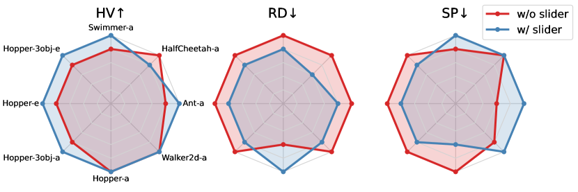
Ablation of Sliding Guidance We conducted an ablation study of the sliding guidance mechanism on 9 tasks within Narrow datasets. The results are presented in the radar chart in fig. 5. We found that in most tasks, MODULI with slider exhibits higher HV and lower RD, indicating leading performance in MO tasks. At the same time, the presence or absence of the slider has little impact on SP performance, indicating that sliding guidance distribution does not impair the ability to express the ID preferences. Besides, we visualized the empirical Pareto front in fig. 5 for Hopper-Narrow dataset. The sliding bootstrap mechanism significantly extends the Pareto set of OOD preference regions, exhibiting better generalization. Due to space limits, we provide more comparative experiments on the different guidance mechanisms (CG, CG+CFG) in appendix G.

5.3 Comparison of Normalization Methods

Table 3: Comparison of normalization on Complete datasets. (NP: Neighborhood Preference, PP: Preference Predicted)

	Env	Metrics	NP Norm	PP Norm	Global Norm
Amateur	Hopper	HV ( $\times 10^{7}$ )	1.98±.02	1.94±.01	1.58±.02
	Hopper	SP ( $\times 10^{5}$ )	0.21±.06	0.24±.06	0.12±.03
	Walker2d	HV ( $\times 10^{6}$ )	5.03±.00	4.94±.00	4.02±.01
	Walker2d	SP ( $\times 10^{4}$ )	0.20±.01	0.31±.01	0.04±.01
Expert	Hopper	HV ( $\times 10^{7}$ )	2.07±.00	2.07±.01	1.48±.02
	Hopper	SP ( $\times 10^{5}$ )	0.14±.04	0.12±.02	2.69±1.97
	Walker2d	HV ( $\times 10^{6}$ )	5.20±.00	5.18±.00	2.70±.04
	Walker2d	SP ( $\times 10^{4}$ )	0.11±.01	0.17±.01	5.11±6.88

We compared the impact of different return regularization methods on MODULI’s performance on the Complete dataset. As shown in table 3, Neighborhood Preference Normalization (NP Norm) consistently has the highest HV performance. On the expert dataset, both NP Norm and PP Norm exhibit very similar HV values, as they can accurately estimate the highest return corresponding to each preference, whether through prediction or neighborhood analysis. However, on the amateur dataset, PP Norm fails to predict accurately, resulting in lower performance. We also noted that the naive method of Global Norm fails to approximate the Pareto front well, but in some datasets, it achieved denser solutions (small SP). We believe this is because the Global Norm produced inaccurate and homogenized guiding information, leading to different preferences for similar solutions, and resulting in dense but low-quality solutions. We refer to appendix C for in-depth visual analysis.

6 Conclusion

In this paper, we propose MODULI, a diffusion planning framework along with two corresponding multi-objective normalization schemes, enabling preference-return condition-guided trajectory generation for decision-making. To achieve better generalization in OOD preferences, MODULI includes a sliding guidance mechanism, training an additional slider adapter for active distribution adjustment. We conduct extensive experiments on Complete, Shattered, and Narrow types of datasets, demonstrating the superior expressive and generalization capabilities of MODULI. The results show that MODULI is an excellent Pareto front approximator, capable of expanding the Pareto front and obtaining advanced and dense solutions. But there are still limitations such as experiments being conducted only in structured state space and continuous actions. We hope to extend it to multi-objective tasks with image inputs, further enhancing its generalization ability. Additionally, nonlinear preference spaces may present new challenges.

References

[1] Anurag Ajay, Yilun Du, Abhi Gupta, Joshua B. Tenenbaum, Tommi S. Jaakkola, and Pulkit Agrawal. Is conditional generative modeling all you need for decision making? In The Eleventh International Conference on Learning Representations, ICLR, 2023.
[2] Lucas N Alegre, Ana LC Bazzan, Diederik M Roijers, Ann Nowé, and Bruno C da Silva. Sample-efficient multi-objective learning via generalized policy improvement prioritization. arXiv preprint arXiv:2301.07784, 2023.
[3] Lucas Nunes Alegre. Towards sample-efficient multi-objective reinforcement learning. In AAMAS, pages 2970–2972, 2023.
[4] Junyong Bae, Jae Min Kim, and Seung Jun Lee. Deep reinforcement learning for a multi-objective operation in a nuclear power plant. Nuclear Engineering and Technology, 55(9):3277–3290, 2023.
[5] Krishnendu Chatterjee, Rupak Majumdar, and Thomas A Henzinger. Markov decision processes with multiple objectives. In STACS 2006: 23rd Annual Symposium on Theoretical Aspects of Computer Science, Marseille, France, February 23-25, 2006. Proceedings 23, pages 325–336. Springer, 2006.
[6] Lili Chen, Kevin Lu, Aravind Rajeswaran, Kimin Lee, Aditya Grover, Misha Laskin, Pieter Abbeel, Aravind Srinivas, and Igor Mordatch. Decision transformer: Reinforcement learning via sequence modeling. Advances in neural information processing systems, 34:15084–15097, 2021.
[7] Cheng Chi, Siyuan Feng, Yilun Du, Zhenjia Xu, Eric Cousineau, Benjamin Burchfiel, and Shuran Song. Diffusion policy: Visuomotor policy learning via action diffusion. In Robotics: Science and Systems XIX, 2023.
[8] Prafulla Dhariwal and Alexander Nichol. Diffusion models beat gans on image synthesis. Advances in neural information processing systems, 34:8780–8794, 2021.
[9] Zibin Dong, Jianye Hao, Yifu Yuan, Fei Ni, Yitian Wang, Pengyi Li, and Yan Zheng. Diffuserlite: Towards real-time diffusion planning. arXiv preprint arXiv:2401.15443, 2024.
[10] Zibin Dong, Yifu Yuan, Jianye HAO, Fei Ni, Yao Mu, YAN ZHENG, Yujing Hu, Tangjie Lv, Changjie Fan, and Zhipeng Hu. Aligndiff: Aligning diverse human preferences via behavior-customisable diffusion model. In The Twelfth International Conference on Learning Representations, ICLR, 2023.
[11] Yilun Du, Shuang Li, and Igor Mordatch. Compositional visual generation with energy based models. Advances in Neural Information Processing Systems, 33:6637–6647, 2020.
[12] Scott Emmons, Benjamin Eysenbach, Ilya Kostrikov, and Sergey Levine. Rvs: What is essential for offline rl via supervised learning? arXiv preprint arXiv:2112.10751, 2021.
[13] Florian Felten, Lucas N Alegre, Ann Nowe, Ana Bazzan, El Ghazali Talbi, Grégoire Danoy, and Bruno C da Silva. A toolkit for reliable benchmarking and research in multi-objective reinforcement learning. In Advances in Neural Information Processing Systems, 2024.
[14] Rohit Gandikota, Joanna Materzynska, Tingrui Zhou, Antonio Torralba, and David Bau. Concept sliders: Lora adaptors for precise control in diffusion models. arXiv preprint arXiv:2311.12092, 2023.
[15] Xiangming Gu, Chao Du, Tianyu Pang, Chongxuan Li, Min Lin, and Ye Wang. On memorization in diffusion models. arXiv preprint arXiv:2310.02664, 2023.
[16] Philippe Hansen-Estruch, Ilya Kostrikov, Michael Janner, Jakub Grudzien Kuba, and Sergey Levine. Idql: Implicit q-learning as an actor-critic method with diffusion policies. arXiv preprint arXiv:2304.10573, 2023.
[17] Conor F Hayes, Roxana Rădulescu, Eugenio Bargiacchi, Johan Källström, Matthew Macfarlane, Mathieu Reymond, Timothy Verstraeten, Luisa M Zintgraf, Richard Dazeley, Fredrik Heintz, et al. A practical guide to multi-objective reinforcement learning and planning. Autonomous Agents and Multi-Agent Systems, 36(1):26, 2022.
[18] Haoran He, Chenjia Bai, Kang Xu, Zhuoran Yang, Weinan Zhang, Dong Wang, Bin Zhao, and Xuelong Li. Diffusion model is an effective planner and data synthesizer for multi-task reinforcement learning. Advances in neural information processing systems, NIPS, 36, 2024.
[19] Jonathan Ho, Ajay Jain, and Pieter Abbeel. Denoising diffusion probabilistic models. Advances in neural information processing systems, 33:6840–6851, 2020.
[20] Jonathan Ho and Tim Salimans. Classifier-free diffusion guidance. arXiv preprint arXiv:2207.12598, 2022.
[21] Wei Hung, Bo-Kai Huang, Ping-Chun Hsieh, and Xi Liu. Q-pensieve: Boosting sample efficiency of multi-objective rl through memory sharing of q-snapshots. The Tenth International Conference on Learning Representations, 2022.
[22] Michael Janner, Yilun Du, Joshua Tenenbaum, and Sergey Levine. Planning with diffusion for flexible behavior synthesis. In Proceedings of the 39th International Conference on Machine Learning, ICML, 2022.
[23] Zahra Kadkhodaie, Florentin Guth, Eero P Simoncelli, and Stéphane Mallat. Generalization in diffusion models arises from geometry-adaptive harmonic representation. The Twelve International Conference on Learning Representations, ICLR, 2024.
[24] Diederik Kingma, Tim Salimans, Ben Poole, and Jonathan Ho. Variational diffusion models. Advances in neural information processing systems, 34:21696–21707, 2021.
[25] Aviral Kumar, Aurick Zhou, George Tucker, and Sergey Levine. Conservative q-learning for offline reinforcement learning. Advances in Neural Information Processing Systems, 33:1179–1191, 2020.
[26] Changjian Li and Krzysztof Czarnecki. Urban driving with multi-objective deep reinforcement learning. arXiv preprint arXiv:1811.08586, 2018.
[27] Puheng Li, Zhong Li, Huishuai Zhang, and Jiang Bian. On the generalization properties of diffusion models. Advances in Neural Information Processing Systems, 36, 2024.
[28] Qian Lin, Chao Yu, Zongkai Liu, and Zifan Wu. Policy-regularized offline multi-objective reinforcement learning. AAMAS, 2024.
[29] Chunming Liu, Xin Xu, and Dewen Hu. Multiobjective reinforcement learning: A comprehensive overview. IEEE Transactions on Systems, Man, and Cybernetics: Systems, 45(3):385–398, 2014.
[30] Ilya Loshchilov and Frank Hutter. Decoupled weight decay regularization. arXiv preprint arXiv:1711.05101, 2017.
[31] Cong Lu, Philip Ball, Yee Whye Teh, and Jack Parker-Holder. Synthetic experience replay. Advances in Neural Information Processing Systems, NIPS, 36, 2024.
[32] H. Lu, D. Herman, and Y. Yu. Multi-objective reinforcement learning: Convexity, stationarity and pareto optimality. In ICLR, 2023.
[33] Haoye Lu, Daniel Herman, and Yaoliang Yu. Multi-objective reinforcement learning: Convexity, stationarity and pareto optimality. In The Eleventh International Conference on Learning Representations, 2023.
[34] Diganta Misra. Mish: A self regularized non-monotonic neural activation function. arXiv preprint arXiv:1908.08681, 2019.
[35] S. Natarajan and P. Tadepalli. Dynamic preferences in multi-criteria reinforcement learning. In ICML, 2005.
[36] Fei Ni, Jianye Hao, Yao Mu, Yifu Yuan, Yan Zheng, Bin Wang, and Zhixuan Liang. MetaDiffuser: Diffusion model as conditional planner for offline meta-RL. In Proceedings of the 40th International Conference on Machine Learning, ICML, 2023.
[37] Alexander Quinn Nichol and Prafulla Dhariwal. Improved denoising diffusion probabilistic models. In International conference on machine learning, pages 8162–8171. PMLR, 2021.
[38] Diederik M Roijers, Peter Vamplew, Shimon Whiteson, and Richard Dazeley. A survey of multi-objective sequential decision-making. Journal of Artificial Intelligence Research, 48:67–113, 2013.
[39] Diederik M Roijers, Shimon Whiteson, Ronald Brachman, and Peter Stone. Multi-objective decision making. Springer, 2017.
[40] Nataniel Ruiz, Yuanzhen Li, Varun Jampani, Yael Pritch, Michael Rubinstein, and Kfir Aberman. Dreambooth: Fine tuning text-to-image diffusion models for subject-driven generation. In Proceedings of the IEEE/CVF conference on computer vision and pattern recognition, pages 22500–22510, 2023.
[41] Jiaming Song, Chenlin Meng, and Stefano Ermon. Denoising diffusion implicit models. International Conference on Learning Representations, 2021.
[42] Yang Song, Jascha Sohl-Dickstein, Diederik P Kingma, Abhishek Kumar, Stefano Ermon, and Ben Poole. Score-based generative modeling through stochastic differential equations. International Conference on Learning Representations, 2021.
[43] Philip S Thomas, Joelle Pineau, Romain Laroche, et al. Multi-objective spibb: Seldonian offline policy improvement with safety constraints in finite mdps. Advances in Neural Information Processing Systems, 34:2004–2017, 2021.
[44] Zhendong Wang, Jonathan J Hunt, and Mingyuan Zhou. Diffusion policies as an expressive policy class for offline reinforcement learning. In The Eleventh International Conference on Learning Representations, ICLR, 2023.
[45] Runzhe Wu, Yufeng Zhang, Zhuoran Yang, and Zhaoran Wang. Offline constrained multi-objective reinforcement learning via pessimistic dual value iteration. Advances in Neural Information Processing Systems, 34:25439–25451, 2021.
[46] Zhou Xian, Nikolaos Gkanatsios, Theophile Gervet, Tsung-Wei Ke, and Katerina Fragkiadaki. Chaineddiffuser: Unifying trajectory diffusion and keypose prediction for robotic manipulation. In 7th Annual Conference on Robot Learning, 2023.
[47] Jie Xu, Yunsheng Tian, Pingchuan Ma, Daniela Rus, Shinjiro Sueda, and Wojciech Matusik. Prediction-guided multi-objective reinforcement learning for continuous robot control. In International conference on machine learning, 2020.
[48] Runzhe Yang, Xingyuan Sun, and Karthik Narasimhan. A generalized algorithm for multi-objective reinforcement learning and policy adaptation. Advances in neural information processing systems, 32, 2019.
[49] Sherry Yang, Yilun Du, Seyed Kamyar Seyed Ghasemipour, Jonathan Tompson, Leslie Pack Kaelbling, Dale Schuurmans, and Pieter Abbeel. Learning interactive real-world simulators. In The Twelfth International Conference on Learning Representations, ICLR, 2024.
[50] Baiting Zhu, Meihua Dang, and Aditya Grover. Scaling pareto-efficient decision making via offline multi-objective rl. The Eleventh International Conference on Learning Representations, 2023.
[51] Zhengbang Zhu, Hanye Zhao, Haoran He, Yichao Zhong, Shenyu Zhang, Yong Yu, and Weinan Zhang. Diffusion models for reinforcement learning: A survey. arXiv preprint arXiv:2311.01223, 2023.

Appendix A Dataset and Baselines

A.1 D4MORL Benchmark

In this paper, we use the Datasets for Multi-Objective Reinforcement Learning (D4MORL) [50] for experiments, a large-scale benchmark for Offline MORL. This benchmark consists of offline trajectories from 6 multi-objective MuJoCo environments, including 5 environments with 2 objectives each, namely MO-Ant, MO-HalfCheetah, MO-Hopper, MO-Swimmer, MO-Walker2d, and one environment with three objectives: MO-Hopper-3obj. The objectives in each environment are conflicting, such as high-speed running and energy saving. In D4MORL, Each environment uses PGMORL’s [47] behavioral policies for data collection. PGMORL trains a set of policies using evolutionary algorithms to approximate the Pareto front, which can map to the closest preference in the preference set for any given preference. Therefore, in D4MORL, two different quality datasets are defined: the Expert Dataset, which is collected entirely using the best preference policies in PGMORL for decision making, and the Amateur Dataset, which has a probability $P$ of using perturbed preference policies and a probability $1-p$ of being consistent with the expert dataset, with $p=0.65$ . We can simply consider the Amateur Dataset as a relatively lower quality dataset with random perturbations added to the Expert Dataset. Each trajectory in the D4MORL dataset is represented as: $\tau=[\bm{\omega},\bm{s}_{0},\bm{a}_{0},\bm{r}_{0},\cdots,\bm{s}_{T},\bm{a}_{T},\bm{r}_{T}]$ , where $T$ is episode length.

A.2 Complete, Shattered and Narrow Datasets

In this section, we provide a detailed description of how three different levels of datasets are collected, and what properties of the algorithm they are used to evaluate respectively:

•

Complete datasets i.e. the original version of the D4MORL datasets, cover a wide range of preference distributions with fewer OOD preference regions. These datasets primarily evaluate the expressive ability of algorithms and require deriving the correct solution based on diverse preferences.
•

Shattered datasets simulate the scenario where the preference distribution in the dataset is incomplete, resulting in areas with missing preferences. This kind of dataset primarily evaluates the interpolation OOD generalization ability of algorithms, aiming for strong generalization capability when encountering unseen preferences with some lacking preferences. Specifically, the Shattered dataset removes part of the trajectories from the Complete dataset, creating $n$ preference-missing regions, which account for $m\%$ of the trajectories. If the total number of trajectories in the dataset is $N$ , then a total of $n_{\text{lack}}=N*m\%$ trajectories are removed. First, all trajectories in the dataset are sorted based on the first dimension of their preferences $\bm{\omega}$ , then $n$ points are selected at equal intervals according to the sorting results. Centered on these $n$ points, an equal number of $n_{\text{lack}}/n$ trajectories around each point are uniformly deleted. In this paper, $m,n$ are fixed to 30, and 3, respectively.
•

The role of Narrow datasets is similar to Shattered datasets but mainly evaluates the extrapolation OOD generalization ability of algorithms. If we need to remove a total of $m\%$ of the trajectories, we can obtain the Narrow dataset with a narrow preference distribution by removing the same amount, $m/2\%$ , from both ends of the sorted Complete dataset. In this paper, $m$ is fixed to 30.

A.3 Baselines

In this paper, we compare with various strong baselines: MODT(P) [6], MORvS(P) [12], BC(P), and MOCQL(P) [25], all of which are well-studied baselines under the PEDA [50], representing different paradigms of learning methods. All baselines were trained using the default hyperparameters and official code as PEDA. MODT(P) extends DT architectures to include preference tokens and vector-valued returns. Additionally, MODT(P) also concatenates $\bm{\omega}$ to state tokens $[\bm{s},\bm{\omega}]$ and action tokens $[\bm{a},\bm{\omega}]$ for training. MORvS(P) and MODT(P) are similar, extending the MLP structure to adapt to MORL tasks. MORvS(P) concatenates the preference with the states and the average RTGs by default as one single input. BC(P) serves as an imitation learning paradigm to train a mapping from states with preference to actions. BC(P) simply uses supervised loss and MLPs as models. MOCQL(P) represents the temporal difference learning paradigm, which learns a preference-conditioned Q-function. Then, MOCQL(P) uses underestimated Q functions for actor-critic learning, alleviating the OOD phenomenon in Offline RL.

A.4 Evaluation Metrics

In MORL, our goal is to train a policy to approximate the true Pareto front. While we do not know the true Pareto front for many problems, we can define metrics for evaluating the performance of different algorithms. Here We define several metrics for evaluation based on the empirical Pareto front $P$ , namely Hypervolume (HV), Sparsity (SP), and Return Deviation (RD), we provide formal definitions as below:

Definition 1 (Hypervolume (HV)).

Hypervolume $\mathcal{H}(P)$ measures the space enclosed by the solutions in the Pareto front $P$ :

\mathcal{H}(P)=\int_{\mathbb{R}^{n}}{\mathbf{1}_{H(P)}(\bm{z})\mathrm{d}\bm{z}},

where $H(P)=\{\bm{z}\in\mathbb{R}^{n}|\exists i:1\leq i\leq|P|,\bm{r_{0}}\preceq\bm{z}\preceq P(i)\}$ , $\bm{r_{0}}$ is a reference point determined by the environment, $\preceq$ is the dominance relation operator and $\mathbf{1}_{H(P)}$ equals 1 if $\bm{z}\in H(P)$ and 0 otherwise. Higher HV is better, implying empirical Pareto front expansion.

Definition 2 (Sparsity (SP)).

Sparsity $\mathcal{S}(P)$ measures the density of the Pareto front $P$ :

\mathcal{S}(P)=\frac{1}{|P|-1}\sum_{i=1}^{n}\sum_{k=1}^{|P|-1}(\tilde{P}_{i}(k)-\tilde{P}_{i}(k+1))^{2},

where $\tilde{P}_{i}$ represents the sorted list of values of the $i$ -th target in $P$ and $\tilde{P}_{i}(k)$ is the $k$ -th value in $\tilde{P}_{i}$ . Lower SP, indicating a denser approximation of the Pareto front, is better.

Definition 3 (Return Deviation (RD)).

The return deviation $\mathcal{R}(O)$ measures the discrepancy between the solution set $O$ in the out-of-distribution preference region and the maximum predicted value:

\mathcal{R}(O)=\frac{1}{|O|}\sum_{k=1}^{|O|}\|O(k)-\bm{R}_{\psi}(\bm{\omega}_{O(k)})\|_{2}^{2}

where $\bm{R}_{\psi}$ is a generalized return predictor to predict the maximum expected return achievable for a given preference $\bm{\omega}$ . To accurately evaluate RD, we consistently train this network $\bm{R}_{\psi}$ using the Complete-Expert dataset, as shown in eq. 7. In this way, for any preference of a missing dataset, we can predict and know the oracle’s solution. Please note that $\bm{R}_{\psi}$ here is only used to evaluate algorithm performance and is unrelated to the Preference Predicted Normalization method in MODULI. $\bm{\omega}_{O(k)}$ is the corresponding preference of $O(k)$ . A lower RD is better, as it indicates that the performance of the solution is closer to the predicted maximum under OOD preference, suggesting better generalization ability.

Appendix B Implementation Details

In this section, we provide the implementation details of MODULI.

•

We utilize a DiT structure similar to AlignDiff [10] as the backbone for all diffusion models, with an embedding dimension of 128, 6 attention heads, and 4 DiT blocks. We use a 2-layer MLP for condition embedding with inputs $[\bm{\omega},\bm{g}]$ . For Preference Prediction Normalization, we use a 3-layer MLP to predict the maximum expected RTG for given preferences. For Neighborhood Preference Normalization, The neighborhood hyperparameter $\epsilon$ is fixed at $1e-3$ for 2-obj experiments and $3e-3$ for 3-obj experiments. For the slider adapter, we use a DiT network that is the same as the diffusion backbone of the slider. We observe that using the Mish activation [34] is more stable in OOD preference regions compared to the ReLU activation, which tends to diverge quickly. Finally, the model size of MODULI is around 11M.
•

All models utilize the AdamW [30] optimizer with a learning rate of $2e-4$ and weight decay of $1e-5$ . We perform a total of 200K gradient updates with a batch size of 64 for all experiments. We employ the exponential moving average (EMA) model with an ema rate of $0.995$ .
•

For all diffusion models, we use a continuous linear noise schedule [37] for $\alpha_{s}$ and $\sigma_{s}$ . We employ DDIM [41] for denoising generation and use a sampling step of $10$ . For all tasks, we use a sampling temperature of $0.5$ .
•

The length of the planning horizon $H$ of the diffusion model should be adequate to capture the agent’s behavioral preferences. Therefore, MODULI uses different planning horizons for different environments according to their properties. For Hopper and Walker2d tasks, we use a planning horizon of $32$ ; for other tasks, we use a planning horizon of $4$ . For conditional sampling, we use guidance weight $w$ as $1.5$ .
•

The inverse dynamic model is implemented as a 3-layer MLP. The first two layers consist of a Linear layer followed by a Mish [34] activation and a LayerNorm. And, the final layer is followed by a Tanh activation. This model utilizes the AdamW optimizer and is trained for 500K gradient steps.
•

For all 2-obj tasks, we evaluate the model on 501 preferences uniformly distributed in the preference space. For all 3-obj tasks, we evaluate the model on 325 preferences uniformly distributed in the preference space. We perform three rounds of evaluation with different seeds and report the mean and standard deviation. Please note that in the Complete dataset, we default to not using the slider adapter for sliding guidance because there is no OOD preference.

Compute Resources

We conducted our experiments on an Intel(R) Xeon(R) Platinum 8171M CPU @ 2.60GHz processor based system. The system consists of 2 processors, each with 26 cores running at 2.60GHz (52 cores in total) with 32KB of L1, 1024 KB of L2, 40MB of unified L3 cache, and 250 GB of memory. Besides, we use 8 Nvidia RTX3090 GPUs to facilitate the training procedure. The operating system is Ubuntu 18.04.

Appendix C In-depth Analysis of Different Normalization Methods

As shown in fig. 6, we visualize the trajectory returns of the Walker2d-amateur-Complete dataset after applying different normalization methods. In order to achieve refined guided generation, we require consistency between the training objectives and the sampling objectives, meaning the sampling objectives should correspond to high-quality trajectories in the dataset. A simple Global Normalization fails to achieve this, as it cannot identify a definitive high-return guiding objective that matches the return distribution of dataset. Setting the return to $\bm{1}^{\bm{n}}$ may be unachievable for Global Normalization. On the contrary, Preference Predicted Normalization (PPN) and Neighborhood Preference Normalization (NPN) successfully normalize the trajectories in the dataset into distinctly different trajectories. High-quality trajectories that conform to preferences are clustered around $\bm{1}^{\bm{n}}$ , and trajectories points farther from $\bm{1}^{\bm{n}}$ represent lower vector returns. Note that at this time, the training objective and the sampling objective are fully aligned. Compared with NPN, the PPN method uses neural networks to predict the maximum expected RTG for each preference, facing prediction errors in low-quality datasets (e.g. amateur dataset). After PPN process using $\bm{g}_{\tau}/\bm{g}_{\text{max}}(\bm{\omega})$ , a small number of trajectories even slightly exceed $\bm{1}^{\bm{n}}$ , indicating that $\bm{R}_{\psi}(\bm{\omega})$ fails to accurately predict the maximum expected return. This ultimately causes the guidance target $\bm{1}^{\bm{n}}$ used in the deployment phase to mismatch the target corresponding to the high trajectory return in training, resulting in a suboptimal policy. The NPN method can achieve accurate normalization for multi-objective targets, significantly distinguishing the quality of trajectories in the dataset, while ensuring that the sampling targets during the training phase and the deployment phase are consistent.

Appendix D Proofs for Sliding Guidance

In this section, we provide a derivation process of the sliding guidance mechanism, which enables controlled continuous target distribution adjustment. Given a trained diffusion model $p_{\theta}$ and condition $c$ , and define the adapter as $p_{\theta^{*}}$ , our goal is to obtain $\theta^{*}$ that increase the likelihood of attribute $c_{+}$ while decrease the likelihood of “opposite” attribute $c_{-}$ when conditioned on $c$ :

p_{\theta}\left(\bm{x}^{0}(\tau)\mid c\right)\leftarrow p_{\theta}\left(\bm{x}^{0}(\tau)\mid c\right)\left(\frac{p_{\theta^{*}}\left(c_{+}\mid\bm{x}^{0}(\tau)\right)}{p_{\theta^{*}}\left(c_{-}\mid\bm{x}^{0}(\tau)\right)}\right)^{\eta}

(14)

where $p_{\theta}\left(\bm{x}^{0}(\tau)\mid c\right)$ represents the distribution generated by the original diffusion model $\theta$ when conditioned on $c$ . According to the Bayesian formula $p\left(c_{+}\mid\bm{x}^{0}(\tau)\right)=\frac{p\left(\bm{x}^{0}(\tau)\mid c_{+}\right)p\left(c_{+}\right)}{p\left(\bm{x}^{0}(\tau)\right)}$ , the gradient of the log probability $\nabla\log{[p_{\theta}\left(\bm{x}^{0}(\tau)\mid c\right)\left(\frac{p_{\theta^{*}}\left(c_{+}\mid\bm{x}^{0}(\tau)\right)}{p_{\theta^{*}}\left(c_{-}\mid\bm{x}^{0}(\tau)\right)}\right)^{\eta}]}$ can be expanded to:

\nabla\log{[p_{\theta}\left(\bm{x}^{0}(\tau)\mid c\right)\left(\frac{p_{\theta^{*}}\left(\bm{x}^{0}(\tau)\mid c_{+}\right)p\left(c_{+}\right)}{p_{\theta^{*}}\left(\bm{x}^{0}(\tau)\mid c_{-}\right)p\left(c_{-}\right)}\right)^{\eta}]}

(15)

which is proportional to:

\nabla\log{p_{\theta}\left(\bm{x}^{0}(\tau)\mid c\right)}+\eta\left(\nabla\log{p_{\theta^{*}}\left(\bm{x}^{0}(\tau)\mid c_{+}\right)}-\nabla\log{p_{\theta^{*}}\left(\bm{x}^{0}(\tau)\mid c_{-}\right)}\right)

(16)

Based on the reparametrization trick of [19], we can introduce a time-varying noising process and express each score (gradient of log probability) as a denoising prediction $\epsilon\left(\bm{x}^{t},c,t\right)$ , thus eq. 16 is equivalent to modifying the noise prediction model:

\epsilon_{\theta}\left(\bm{x}^{t},c,t\right)\leftarrow\epsilon_{\theta}\left(\bm{x}^{t},c,t\right)+\eta\left(\epsilon_{\theta^{*}}\left(\bm{x}^{t},c_{+},t\right)-\epsilon_{\theta^{*}}\left(\bm{x}^{t},c_{-},t\right)\right)

(17)

Appendix E Pseudo Code

In this section, we explain the training and inference process of MODULI in pseudo code. MODULI first trains a standard diffusion model for conditional generation; then, we freeze the parameters of this model and use an additional network, the slider, to learn the latent direction of policy shift. Finally, we jointly use the original diffusion and the slider to achieve controllable preference generalization. The pseudo code are given below.

Training Process of MODULI

The training process of the MODULI consists of two parts: the training of the diffusion model and the training of the slider adapter, which are described in Algorithms 1 and 2, respectively. Given a normalized dataset $D_{g}$ containing trajectories of states $\bm{s}$ , normalized RTG $\bm{g}$ and preferences $\bm{\omega}$ , MODULI first trains a diffusion planner $\theta$ :

Algorithm 1 Diffusion Training

0: normalized dataset

\mathcal{D}_{\bm{g}}

, diffusion model

\theta

while not done do

(\bm{x}^{0},\bm{\omega},\bm{g})\sim\mathcal{D}_{\bm{g}}

t\sim\text{Uniform}(\{1,\cdots,T\})

\bm{\epsilon}\sim\mathcal{N}(\bm{0},\bm{I})

\mathcal{L}(\theta)=\mathbb{E}_{(\bm{x}^{0},\bm{\omega},\bm{g})\sim\mathcal{D},t\sim U(0,T),\epsilon\sim\mathcal{N}(\bm{0},\bm{I})}\left[\|\bm{\epsilon}_{\theta}(\bm{x}^{t},t,\bm{\omega},\bm{g})-\bm{\epsilon}\|^{2}_{2}\right]

Update

\theta

to minimize

\mathcal{L}(\theta)

end while

After training the diffusion model $\theta$ , we freeze its parameters to prevent any changes when training the slider. At each step, we sample a random preference shift from a uniform distribution $\Delta\bm{\omega}\sim\text{Uniform}(\{-{\Delta\bm{\omega}}^{\text{max}},{\Delta\bm{\omega}}^{\text{max}}\})$ , where ${\Delta\bm{\omega}}^{\text{max}}$ is a preset maximum preference shift to avoid sampling ood preference. In implementation, ${\Delta\bm{\omega}}^{\text{max}}$ is set to $1e-3$ . We then use the diffusion model to sample a pair of predicted noises ( $\epsilon_{\theta}(\bm{x}^{t},t,\bm{\omega}+\Delta{\bm{\omega}},\bm{g}),\epsilon_{\theta}(\bm{x}^{t},t,\bm{\omega}-\Delta\bm{\omega},\bm{g})$ ) whose preferences are positively and negatively shifted, and divide them by the shift value of the preference $2\Delta\bm{\omega}$ to represent the “noise shift caused by unit preference shift”. The slider model is used to explicitly capture this shift. The specific training process and gradient target are detailed below:

Algorithm 2 Slider Training

0: normalized dataset

\mathcal{D}_{\bm{g}}

, pretrained diffusion model

\theta

, slider adapter

\theta^{*}

, preference shift

{\Delta\bm{\omega}}^{\text{max}}

while not done do

(\bm{x}^{0},\bm{\omega},\bm{g})\sim\mathcal{D}

\Delta\bm{\omega}\sim\text{Uniform}(\{-{\Delta\bm{\omega}}^{\text{max}},{\Delta\bm{\omega}}^{\text{max}}\})

t\sim\text{Uniform}(\{1,\cdots,T\})

\bm{\epsilon}\sim\mathcal{N}(\bm{0},\bm{I})

\mathcal{L}(\theta^{*})=\mathbb{E}_{(\bm{\omega},\bm{g},\bm{\Delta\omega})\sim D}\left[\left\|\epsilon_{\theta^{*}}(\bm{x}^{t},t,\bm{\omega},\bm{g})-\frac{[\epsilon_{\theta}(\bm{x}^{t},t,\bm{\omega}+\Delta{\bm{\omega}},\bm{g})-\epsilon_{\theta}(\bm{x}^{t},t,\bm{\omega}-\Delta\bm{\omega},\bm{g})]}{2\Delta\bm{\omega}}\right\|_{2}^{2}\right]

Update

\theta^{*}

to minimize

\mathcal{L}(\theta^{*})

end while

Inference Process of MODULI

During deployment, MODULI utilizes both the diffusion model $\theta$ and the slider $\theta^{*}$ to guide the denoising process. Given a desired preference $\bm{\omega}$ , we first query the closest preference $\bm{\omega}_{0}$ in the dataset. In the $S$ -step denoising process, we expect the distribution of the generated trajectory $\bm{x}$ to gradually shift from the in-distribution preference $\bm{\omega}_{0}$ to the desired preference $\bm{\omega}$ through the guidance of the slider. Formally, we expect that the trajectory $\bm{x}^{\kappa_{i}}$ at the $i$ -th denoising step falls within the distribution $p\left(\bm{x}^{\kappa_{i}}\mid\bm{\omega}_{i},\kappa_{i}\right)$ . After one step of diffusion denoising, it falls within the distribution $p\left(\bm{x}^{\kappa_{i-1}}\mid\bm{\omega}_{i},\kappa_{i-1}\right)$ . Subsequently, after the slider shift, it falls within the distribution $p\left(\bm{x}^{\kappa_{i-1}}\mid\bm{\omega}_{i-1},\kappa_{i-1}\right)$ . The pseudocode for the implementation is provided in algorithm 3:

Algorithm 3 MODULI planning

0: dataset

\mathcal{D}

, diffusion model

\theta

, slider

\theta^{*}

, target preference

\bm{\omega}

, inverse dynamics

h_{\phi}

S

-length sampling sequence

\kappa_{S}

, classifier-free guidance scale

w

\bm{\omega}_{0}\leftarrow\mathop{\arg\min}\limits_{\bm{\omega}_{0}}\|\bm{\omega}-\bm{\omega}_{0}\|_{2}^{2},~{}\bm{\omega}_{0}\in\mathcal{D}

\Delta\bm{\omega}=\bm{\omega}-\bm{\omega_{0}}

while not done do

Observe state

\bm{s}_{t}

; Sample noise from prior distribution

\bm{x^{\kappa_{S}}}\sim\mathcal{N}(\bm{0},\bm{I})

for

i=S,\cdots,1

\bm{\omega_{i}}\leftarrow\bm{\omega_{0}}+\frac{S-i}{S}\Delta\bm{\omega}

\tilde{\epsilon}_{\theta}\leftarrow(1+w)\epsilon_{\theta}(\bm{x^{\kappa_{i}}},\kappa_{i},\bm{\omega}_{i},\bm{1}^{n})-w\epsilon_{\theta}(\bm{x^{\kappa_{i}}},\kappa_{i})

\Delta\tilde{\epsilon}_{\theta^{*}}=\frac{\Delta\bm{\omega}}{S}\epsilon_{\theta^{*}}(\bm{x^{\kappa_{i}}},\kappa_{i},\bm{\omega}_{i},\bm{1}^{n})

\bm{x^{\kappa_{i-1}}}\leftarrow\text{Denoise}(\bm{x^{\kappa_{i}}},\tilde{\epsilon}_{\theta}+\Delta\tilde{\epsilon}_{\theta^{*}})

end for

\text{Extract }\bm{s}_{t},\bm{s}_{t+1}\text{ from }\bm{x^{\kappa_{0}}}

and derive

\bm{a}_{t}=h_{\phi}(s_{t},s_{t+1})

\text{Execute }\bm{a}_{t}

end while

Appendix F Full Results

See table 4, table 5 and table 6 for full results of HV, RD, SP on Complete / Shattered / Narrow datasets.

Table 4: HV and SP performance on full Complete datasets. (B: behavioral policy). The best scores are emphasized in bold.

	Env	Metrics	B	MODT(P)	MORvS(P)	BC(P)	CQL(P)	MODULI
Amateur	Ant	HV ( $\times 10^{6}$ ) $\uparrow$	5.61	5.92±.04	6.07±.02	4.37±.06	5.62±.23	6.08±.03
	Ant	SP ( $\times 10^{4}$ ) $\downarrow$	-	8.72±.77	5.24±.52	25.90±16.40	1.06±.28	0.53±.05
	HalfCheetah	HV ( $\times 10^{6}$ ) $\uparrow$	5.68	5.69±.01	5.77±.00	5.46±.02	5.54±.02	5.76±.00
	HalfCheetah	SP ( $\times 10^{4}$ ) $\downarrow$	-	1.16±.42	0.57±.09	2.22±.91	0.45±.27	0.07±.02
	Hopper	HV ( $\times 10^{7}$ ) $\uparrow$	1.97	1.81±.05	1.76±.03	1.35±.03	1.64±.01	2.01±.01
	Hopper	SP ( $\times 10^{5}$ ) $\downarrow$	-	1.61±.29	3.50±1.54	2.42±1.08	3.30±5.25	0.10±.01
	Swimmer	HV ( $\times 10^{4}$ ) $\uparrow$	2.11	1.67±.22	2.79±.03	2.82±.04	1.69±.93	3.20±.00
	Swimmer	SP ( $\times 10^{0}$ ) $\downarrow$	-	2.87±1.32	1.03±.20	5.05±1.82	8.87±6.24	9.50±.59
	Walker2d	HV ( $\times 10^{6}$ ) $\uparrow$	4.99	3.10±.34	4.98±.01	3.42±.42	1.78±.33	5.06±.00
	Walker2d	SP ( $\times 10^{4}$ ) $\downarrow$	-	164.20±13.50	1.94±.06	53.10±34.60	7.33±5.89	0.25±.03
	Hopper-3obj	HV ( $\times 10^{10}$ ) $\uparrow$	3.09	1.04±.16	2.77±.24	2.42±.18	0.59±.42	3.33±.06
	Hopper-3obj	SP ( $\times 10^{5}$ ) $\downarrow$	-	10.23±2.78	1.03±.11	0.87±.29	2.00±1.72	0.10±.00
Expert	Ant	HV ( $\times 10^{6}$ ) $\uparrow$	6.32	6.21±.01	6.36±.02	4.88±.17	5.76±.10	6.39±.02
	Ant	SP ( $\times 10^{4}$ ) $\downarrow$	-	8.26±2.22	0.87±.19	46.20±16.40	0.58±.10	0.79±.12
	HalfCheetah	HV ( $\times 10^{6}$ ) $\uparrow$	5.79	5.73±.00	5.78±.00	5.54±.05	5.63±.04	5.79±.00
	HalfCheetah	SP ( $\times 10^{4}$ ) $\downarrow$	-	1.24±.23	0.67±.05	1.78±.39	0.10±.00	0.07±.00
	Hopper	HV ( $\times 10^{7}$ ) $\uparrow$	2.09	2.00±.02	2.02±.02	1.23±.10	0.33±.39	2.09±.01
	Hopper	SP ( $\times 10^{5}$ ) $\downarrow$	-	16.30±10.60	3.03±.36	52.50±4.88	2.84±2.46	0.09±.01
	Swimmer	HV ( $\times 10^{4}$ ) $\uparrow$	3.25	3.15±.02	3.24±.00	3.21±.00	3.22±.08	3.24±.00
	Swimmer	SP ( $\times 10^{0}$ ) $\downarrow$	-	15.00±7.49	4.39±.07	4.50±.39	13.60±5.31	4.43±.38
	Walker2d	HV ( $\times 10^{6}$ ) $\uparrow$	5.21	4.89±.05	5.14±.01	3.74±.11	3.21±.32	5.20±.00
	Walker2d	SP ( $\times 10^{4}$ ) $\downarrow$	-	0.99±.44	3.22±.73	75.60±52.30	6.23±10.70	0.11±.01
	Hopper-3obj	HV ( $\times 10^{10}$ ) $\uparrow$	3.73	3.38±.05	3.42±.10	2.29±.07	0.78±.24	3.57±.02
	Hopper-3obj	SP ( $\times 10^{5}$ ) $\downarrow$	-	1.40±.44	2.72±1.93	0.72±.09	2.60±3.14	0.07±.00

Table 5: HV, RD and SP performance on full Expert-Shattered and Expert-Narrow datasets. The best scores are emphasized in bold.

	Env	Metrics	MODT(P)	MORvS(P)	BC(P)	MODULI
Expert-Shattered	Ant	HV ( $\times 10^{6}$ ) $\uparrow$	5.88±.02	6.38±.01	4.76±.05	6.39±.01
		RD ( $\times 10^{3}$ ) $\downarrow$	0.71±.03	0.16±.00	0.61±.01	0.14±.01
		SP ( $\times 10^{4}$ ) $\downarrow$	2.22±.50	0.75±.13	5.16±1.18	0.53±.13
	HalfCheetah	HV ( $\times 10^{6}$ ) $\uparrow$	5.69±.00	5.73±.00	5.66±.00	5.78±.00
		RD ( $\times 10^{3}$ ) $\downarrow$	0.18±.00	0.10±.00	0.28±.00	0.07±.00
		SP ( $\times 10^{4}$ ) $\downarrow$	0.18±.01	0.15±.02	0.34±.03	0.11±.02
	Hopper	HV ( $\times 10^{7}$ ) $\uparrow$	1.95±.03	2.06±.01	1.49±.01	2.07±.00
		RD ( $\times 10^{3}$ ) $\downarrow$	1.42±.00	1.10±.04	3.92±.11	0.22±.06
		SP ( $\times 10^{5}$ ) $\downarrow$	0.85±.27	0.20±.06	2.58±1.01	0.11±.01
	Swimmer	HV ( $\times 10^{4}$ ) $\uparrow$	3.20±.00	3.24±.00	3.19±.00	3.24±.00
		RD ( $\times 10^{2}$ ) $\downarrow$	0.38±.00	0.16±.00	0.07±.00	0.06±.00
		SP ( $\times 10^{0}$ ) $\downarrow$	15.50±.33	7.36±.81	9.05±.30	5.79±.43
	Walker2d	HV ( $\times 10^{6}$ ) $\uparrow$	5.01±.01	5.14±.01	3.47±.12	5.20±.00
		RD ( $\times 10^{3}$ ) $\downarrow$	0.86±.01	0.65±.02	1.72±.01	0.15±.01
		SP ( $\times 10^{4}$ ) $\downarrow$	0.49±.03	0.27±.04	16.61±13.78	0.12±.01
	Hopper-3obj	HV ( $\times 10^{10}$ ) $\uparrow$	2.83±.06	3.28±.07	1.95±.16	3.43±.02
		RD ( $\times 10^{3}$ ) $\downarrow$	1.60±.01	1.60±.02	3.21±.01	1.28±.03
		SP ( $\times 10^{5}$ ) $\downarrow$	0.09±.01	0.06±.00	0.17±.06	0.10±.01
Expert-Narrow	Ant	HV ( $\times 10^{6}$ ) $\uparrow$	5.05±.08	6.06±.00	4.90±.02	6.36±.00
		RD ( $\times 10^{3}$ ) $\downarrow$	0.98±.01	0.37±.03	0.78±.03	0.25±.01
		SP ( $\times 10^{4}$ ) $\downarrow$	0.88±.41	0.79±.11	1.56±.28	0.80±.25
	HalfCheetah	HV ( $\times 10^{6}$ ) $\uparrow$	5.04±.00	5.46±.01	4.88±.02	5.76±.00
		RD ( $\times 10^{3}$ ) $\downarrow$	0.43±.00	0.29±.00	0.44±.00	0.17±.00
		SP ( $\times 10^{4}$ ) $\downarrow$	0.04±.00	0.05±.00	0.02±.00	0.04±.00
	Hopper	HV ( $\times 10^{7}$ ) $\uparrow$	1.85±.02	1.98±.00	1.29±.01	2.04±.01
		RD ( $\times 10^{3}$ ) $\downarrow$	4.24±.02	1.37±.05	3.83±.05	2.42±.05
		SP ( $\times 10^{5}$ ) $\downarrow$	0.34±.07	0.16±.02	0.59±.24	0.25±.05
	Swimmer	HV ( $\times 10^{4}$ ) $\uparrow$	3.03±.00	3.10±.00	3.06±.00	3.21±.00
		RD ( $\times 10^{2}$ ) $\downarrow$	0.38±.00	0.39±.01	0.19±.00	0.10±.00
		SP ( $\times 10^{0}$ ) $\downarrow$	3.65±.22	4.38±.80	5.53±.20	3.28±.15
	Walker2d	HV ( $\times 10^{6}$ ) $\uparrow$	4.75±.01	4.85±.01	1.88±.95	5.10±.01
		RD ( $\times 10^{3}$ ) $\downarrow$	1.07±.01	1.45±.02	1.88±.00	0.28±.02
		SP ( $\times 10^{4}$ ) $\downarrow$	0.34±.09	0.19±.02	10.76±11.58	0.13±.01
	Hopper-3obj	HV ( $\times 10^{10}$ ) $\uparrow$	3.18±.05	3.32±.00	2.32±.10	3.37±.05
		RD ( $\times 10^{3}$ ) $\downarrow$	2.48±.00	2.24±.02	2.49±.02	2.38±.01
		SP ( $\times 10^{5}$ ) $\downarrow$	0.11±.01	0.22±.02	0.14±.02	0.12±.01

Table 6: HV, RD and SP performance on full Amateur-Shattered and Amateur-Narrow datasets. The best scores are emphasized in bold.

	Env	Metrics	MODT(P)	MORvS(P)	BC(P)	MODULI
Amateur-Shattered	Ant	HV ( $\times 10^{6}$ ) $\uparrow$	5.74±.04	6.09±.01	4.20±.05	6.04±.01
		RD ( $\times 10^{3}$ ) $\downarrow$	0.36±.01	0.13±.03	1.01±.07	0.09±.01
		SP ( $\times 10^{4}$ ) $\downarrow$	2.47±.61	0.79±.14	2.29±1.38	0.63±.23
	HalfCheetah	HV ( $\times 10^{6}$ ) $\uparrow$	5.61±.01	5.74±.00	5.54±.00	5.75±.00
		RD ( $\times 10^{3}$ ) $\downarrow$	0.62±.00	0.11±.00	0.11±.00	0.07±.00
		SP ( $\times 10^{4}$ ) $\downarrow$	0.11±.01	0.09±.01	0.09±.01	0.13±.01
	Hopper	HV ( $\times 10^{7}$ ) $\uparrow$	1.46±.00	1.69±.01	1.63±.00	2.01±.01
		RD ( $\times 10^{3}$ ) $\downarrow$	2.51±.01	1.76±.02	0.99±.06	0.49±.15
		SP ( $\times 10^{5}$ ) $\downarrow$	0.54±.58	0.18±.01	0.11±.05	0.15±.04
	Swimmer	HV ( $\times 10^{4}$ ) $\uparrow$	0.75±.00	2.81±.00	2.81±.00	3.17±.00
		RD ( $\times 10^{2}$ ) $\downarrow$	0.94±.00	0.40±.00	0.35±.00	0.29±.00
		SP ( $\times 10^{0}$ ) $\downarrow$	6.75±.23	1.26±.06	1.89±.05	8.85±.77
	Walker2d	HV ( $\times 10^{6}$ ) $\uparrow$	3.86±.07	4.99±.00	3.42±.02	5.03±.00
		RD ( $\times 10^{3}$ ) $\downarrow$	1.44±.02	0.37±.02	1.18±.01	0.35±.02
		SP ( $\times 10^{4}$ ) $\downarrow$	11.13±3.58	0.20±.03	4.56±.08	0.29±.01
	Hopper-3obj	HV ( $\times 10^{10}$ ) $\uparrow$	1.48±.02	2.84±.04	1.34±.02	3.02±.03
		RD ( $\times 10^{3}$ ) $\downarrow$	2.86±.01	1.29±.01	2.87±.00	1.01±.04
		SP ( $\times 10^{5}$ ) $\downarrow$	0.56±.08	0.13±.01	0.59±.08	0.10±.01
Amateur-Narrow	Ant	HV ( $\times 10^{6}$ ) $\uparrow$	5.17±.03	5.80±.03	4.19±.10	5.88±.03
		RD ( $\times 10^{3}$ ) $\downarrow$	0.77±.01	0.27±.02	1.93±.04	0.53±.00
		SP ( $\times 10^{4}$ ) $\downarrow$	0.43±.10	0.51±.08	4.42±1.44	0.62±.11
	HalfCheetah	HV ( $\times 10^{6}$ ) $\uparrow$	4.29±.00	5.55±.00	5.08±.01	5.71±.00
		RD ( $\times 10^{3}$ ) $\downarrow$	0.98±.01	0.36±.00	0.36±.00	0.35±.00
		SP ( $\times 10^{4}$ ) $\downarrow$	1.02±.44	0.02±.00	0.02±.03	0.06±.02
	Hopper	HV ( $\times 10^{7}$ ) $\uparrow$	1.73±.01	1.69±.01	0.94±.34	1.99±.00
		RD ( $\times 10^{3}$ ) $\downarrow$	1.38±.04	2.88±.08	5.22±.01	1.33±.11
		SP ( $\times 10^{5}$ ) $\downarrow$	0.27±.07	0.25±.03	5.81±8.21	0.22±.06
	Swimmer	HV ( $\times 10^{4}$ ) $\uparrow$	0.66±.03	2.95±.00	2.80±.00	3.15±.00
		RD ( $\times 10^{2}$ ) $\downarrow$	1.14±.00	0.48±.00	0.49±.00	0.45±.00
		SP ( $\times 10^{0}$ ) $\downarrow$	14.25±3.73	1.91±.01	2.95±.08	5.79±.43
	Walker2d	HV ( $\times 10^{6}$ ) $\uparrow$	3.24±..16	4.83±.00	2.83±.01	4.91±.01
		RD ( $\times 10^{3}$ ) $\downarrow$	1.91±.00	1.77±.00	1.87±.00	0.97±.02
		SP ( $\times 10^{4}$ ) $\downarrow$	5.64±3.72	0.22±.01	0.01±.00	0.24±.01
	Hopper-3obj	HV ( $\times 10^{10}$ ) $\uparrow$	1.85±.04	2.27±.05	2.26±.02	2.90±.05
		RD ( $\times 10^{3}$ ) $\downarrow$	2.44±.02	1.60±.02	1.86±.03	1.84±.04
		SP ( $\times 10^{5}$ ) $\downarrow$	3.12±1.21	0.07±.01	0.09±.00	0.12±.02

Appendix G Additional Experiment Results

G.1 Performance with Different Guidance Mechanism

As shown in table 7, we also compare the slider with different guided sampling methods on the expert datasets, namely CG and CG+CFG. Classifier Guidance (CG) requires training an additional classifier $\log p_{\phi}(\bm{\omega},\bm{g}|\bm{x}^{t},t)$ to predict the log probability of exhibiting property. During inference, the classifier’s gradient is used to guide the solver. CG+CFG combines the CG and CFG methods, using preference $\bm{\omega}$ for guidance in the CFG part and RTG classifier $\log p_{\phi}(\bm{g}|\bm{x}^{t},t)$ for guidance in the CG part. We found that the CFG+CG method performs better than the CG method in most environments, indicating that CG is more suitable for guiding trajectories with high returns. However, MODULI w/ slider still demonstrates the best performance in most environments, especially in the HV and RD metrics.

Table 7: HV, RD and SP performance with different guided sampling methods on the expert datasets.

	Env	Metrics	MODULI	CG	CFG+CG
Expert-Narrow	Ant	HV ( $\times 10^{6}$ ) $\uparrow$	6.36±.00	6.23±.03	6.12±.03
		RD ( $\times 10^{3}$ ) $\downarrow$	0.25±.01	0.44±.03	0.85±.03
		SP ( $\times 10^{4}$ ) $\downarrow$	0.80±.25	0.52±.16	0.81±.12
	HalfCheetah	HV ( $\times 10^{6}$ ) $\uparrow$	5.76±.00	5.69±.01	5.76±.00
		RD ( $\times 10^{3}$ ) $\downarrow$	0.17±.00	0.14±.03	0.52±.03
		SP ( $\times 10^{4}$ ) $\downarrow$	0.04±.00	0.47±.03	0.04±.00
	Hopper	HV ( $\times 10^{7}$ ) $\uparrow$	2.04±.01	1.95±.01	2.03±.01
		RD ( $\times 10^{3}$ ) $\downarrow$	2.42±.05	1.11±.14	2.97±.05
		SP ( $\times 10^{5}$ ) $\downarrow$	0.25±.05	0.09±.01	0.09±.02
	Swimmer	HV ( $\times 10^{4}$ ) $\uparrow$	3.21±.00	3.19±.01	3.16±.00
		RD ( $\times 10^{2}$ ) $\downarrow$	0.10±.00	0.16±.01	1.12±.00
		SP ( $\times 10^{0}$ ) $\downarrow$	3.28±.15	23.28±3.56	5.26±.62
	Walker2d	HV ( $\times 10^{6}$ ) $\uparrow$	5.10±.01	5.01±.06	5.08±.00
		RD ( $\times 10^{3}$ ) $\downarrow$	0.28±.02	0.40±.04	0.63±.00
		SP ( $\times 10^{4}$ ) $\downarrow$	0.13±.01	1.27±.32	0.19±.00
	Hopper-3obj	HV ( $\times 10^{10}$ ) $\uparrow$	3.37±.05	2.30±.08	3.34±.03
		RD ( $\times 10^{3}$ ) $\downarrow$	2.38±.01	2.58±.04	2.45±.03
		SP ( $\times 10^{5}$ ) $\downarrow$	0.12±.01	0.11±.01	0.11±.01
Expert-Shattered	Ant	HV ( $\times 10^{6}$ ) $\uparrow$	6.39±.01	6.23±.03	6.36±.03
		RD ( $\times 10^{3}$ ) $\downarrow$	0.14±.01	0.46±.02	0.14±.00
		SP ( $\times 10^{4}$ ) $\downarrow$	0.53±.13	0.54±.13	0.54±.16
	HalfCheetah	HV ( $\times 10^{6}$ ) $\uparrow$	5.78±.00	5.69±.01	5.78±.00
		RD ( $\times 10^{3}$ ) $\downarrow$	0.07±.00	0.37±.00	0.07±.03
		SP ( $\times 10^{4}$ ) $\downarrow$	0.11±.02	0.47±.03	0.12±.01
	Hopper	HV ( $\times 10^{7}$ ) $\uparrow$	2.07±.01	1.95±.01	2.07±.01
		RD ( $\times 10^{3}$ ) $\downarrow$	0.22±.06	0.81±.19	0.23±.03
		SP ( $\times 10^{5}$ ) $\downarrow$	0.11±.01	0.13±.12	0.12±.01
	Swimmer	HV ( $\times 10^{4}$ ) $\uparrow$	3.24±.00	3.19±.01	3.24±.00
		RD ( $\times 10^{2}$ ) $\downarrow$	0.06±.00	0.29±.02	0.04±.00
		SP ( $\times 10^{0}$ ) $\downarrow$	5.79±.43	23.28±3.56	6.78±1.26
	Walker2d	HV ( $\times 10^{6}$ ) $\uparrow$	5.20±.00	5.19±.00	5.01±.06
		RD ( $\times 10^{3}$ ) $\downarrow$	0.15±.01	0.17±.01	0.73±.04
		SP ( $\times 10^{4}$ ) $\downarrow$	0.12±.01	0.12±.01	1.27±.32
	Hopper-3obj	HV ( $\times 10^{10}$ ) $\uparrow$	3.43±.02	2.30±.08	3.39±.02
		RD ( $\times 10^{3}$ ) $\downarrow$	1.28±.03	2.45±.10	1.66±.01
		SP ( $\times 10^{5}$ ) $\downarrow$	0.10±.01	0.12±.01	0.10±.01

G.2 Approximate Pareto Front on all Environments

We present the approximate Pareto front visualization results of MODULI for all environments in fig. 7. MODULI is a good Pareto front approximator, capable of extending the front on the amateur dataset and performing interpolation or extrapolation generalization on the Shattered or Narrow datasets.