Modelling radio luminosity functions of radio-loud AGN by the cosmological evolution of supermassive black holes.

Theoretical arguments have shown that the amount of synchrotron radiation emitted from a scale-invariant jet depends both on the black hole mass and the accretion rate (Falcke & Biermann 1995; Heinz & Sunyaev 2003). The first observational evidence of this dependency was the discovery of the fundamental plane (FP) of black hole activity, which is the relationship between X-ray luminosity, radio luminosity, and black hole mass for low accretion rate black holes, connecting Galactic black holes in X-ray binaries and AGN (Merloni et al. 2003; Falcke et al. 2004). In the FP relation the X-ray emission is considered to be a tracer of the accretion rate, while the radio luminosity is used as a probe for the AGN jet. Many authors have since confirmed the existence of a black hole FP relationship (Körding et al. 2006; Merloni & Heinz 2007; Gültekin et al. 2009; Plotkin et al. 2012; Saikia et al. 2015).

According to the FP relation, the radio luminosity of AGN cores is related to the X-ray luminosity and the black hole (BH) mass, $M$, by (e.g. Merloni et al. 2003; Falcke et al. 2004; Plotkin et al. 2012)

$$\log{\mathcal{L}_{c}}=\xi_{X}\log{L_{X}}+\xi_{M}\log{M}+\beta_{R}\,,$$

(1)

where $\mathcal{L}_{c}$ is the intrinsic (i.e. unbeamed) core luminosity at 5 GHz; $L_{X}$ is the (unabsorbed) X-ray luminosity in the 2–10 keV band (both in unit of erg s^-1); and $\xi_{X},\leavevmode\nobreak\ \xi_{M}$, and $\beta_{R}$ are the correlation coefficients of the FP relation.

The observed correlation coefficients can be compared with the values predicted by theoretical models. These coefficients depend roughly on the accretion flow (if it is radiatively efficient or inefficient) and on the dominant physical process that originates the observed X-rays. Several components can potentially contribute to the X-ray emission: synchrotron and synchrotron self-Compton radiation from the jet; emission from the accretion flow; and inverse Compton scattering of soft disc photons on hot electrons of the corona. Merloni et al. (2003) show how different theoretical models for emission processes can be directly translated into predictions of the FP coefficients in the cases where X-rays are predominantly originated by optically thin synchrotron jet emission or by inverse Compton scattering.

For sources at low accretion rates, the FP relation is well established. Different authors (Merloni et al. 2003; Falcke et al. 2004; Gültekin et al. 2009; Plotkin et al. 2012) have determined it with reasonable agreement of the correlation parameters (with some exceptions; e.g. Bongiorno et al. 2012) and in agreement with theoretical expectations for radiatively inefficient accretion flow models (in particular with the advection dominated accretion flow, ADAF, solution; Merloni et al. 2003). Regardless of the physical explanation, this scaling relation implies that the same mechanism governing the accretion and ejection processes from black holes holds over approximately nine orders of magnitude in mass. For low accretion rate (or LK mode) AGN we adopt the correlation coefficients obtained by Merloni & Heinz (2007, 2008) based on the Merloni et al. (2003) data: $\xi_{X}=0.62$, $\xi_{M}=0.55$, and $\beta_{R}=8.6$, with an intrinsic scatter of 0.6 dex.

When high accretion rate sources are included in the FP relation, the inferred coefficients change and the intrinsic scatter increases. Li et al. (2008) and Dong et al. (2014) explored the FP for samples of radiatively efficient black holes. Dong et al. (2014) considered X-ray binaries and radio-quiet type-1 AGN with Eddington ratio higher than 1%. The correlation coefficients they found are different with respect to low-accretion AGN and compatible with those expected from radiatively efficient accretion disc models: the slope with the X-ray luminosity is steeper ($\xi_{X}\simeq 1.6$) and a small anti-correlation with the black hole mass ($\xi_{M}\sim-0.2$) is found. Very similar results are also found in Li et al. (2008), but only for radio-loud broad-line AGN; their sample also includes radio-quiet broad-line AGN that provide results in agreement with the FP of LK mode sources.

Because of the larger uncertainty in the FP relation for HK mode AGN, the correlation coefficients are not fixed in the model as for LK mode AGN, but considered as free parameters.

It is more convenient for us to write the FP relation (Eq. 1) in terms of the Eddington ratio (i.e. the ratio of the bolometric luminosity $L_{B}$ to the Eddington luminosity $L_{\rm Edd}\simeq 1.26\times 10^{38}\,M/{\,\rm M}_{\odot}$ erg s^-1, $\lambda\equiv L_{B}/L_{\rm Edd}$) as

$$\log{\mathcal{L}_{c}}=\xi_{X}\log{\lambda}+(\xi_{M}+\xi_{X})\log{M}+\beta^{\prime}_{R}\,,$$

(2)

where $\beta^{\prime}_{R}=\beta_{R}+\xi_{X}(38.1+\log{f})-\log(5\times 10^{9})$, and $f=L_{X}/L_{B}$ is the bolometric correction (from Marconi et al. 2004). Standard radio monochromatic luminosities are now considered in Eq. 2 (in units of erg s^-1 Hz^-1).

We impose a continuity condition in the FP relationship at the transition of the LK and HK mode regimes (i.e. at the critical accretion rate of $\lambda_{cr}=0.01$). Under this condition we can write HK mode FP parameters as a function of LK mode ones:

	$\displaystyle\xi_{M}^{HK}$	$\displaystyle=$	$\displaystyle\xi_{M}^{LK}+\Delta\xi_{X},$
	$\displaystyle\beta_{R}^{HK}$	$\displaystyle=$	$\displaystyle\beta_{R}^{LK}+\Delta\xi_{X}(38.1+\log\lambda_{cr}+\log f)\,,$		(3)

where $\Delta\xi_{X}=\xi_{X}^{LK}-\xi_{X}^{HK}$. The first equation is obtained by requiring the continuity condition to be valid for each SMBH mass. Thus, if the FP relation is fixed for LK mode AGN, only the coefficient $\xi^{HK}_{X}$ is needed to compute $\mathcal{L}^{HK}_{c}$.

Once the FP relationship is established it is easy to extract the intrinsic luminosity function of AGN cores at 5 GHz (i.e. $\Phi(\mathcal{L}_{c})$²²2Hereafter luminosity functions, mass functions, and Eddington ratio distributions are always defined by logarithmic intervals. The redshift dependence is ignored at the moment.) as a function of the mass function $\Phi_{AGN}(M)$ and the Eddington ratio distribution $P(\lambda|M)$ of active SMBHs. For sources in the $X$ mode (with $X=LK$ or $HK$) we have

	$\displaystyle\Phi_{X}(\mathcal{L}_{c})$	$\displaystyle=$	$\displaystyle\int d\log(M)d\log(\lambda)\,\Phi_{X}(\mathcal{L}_{c},M,\lambda)=$		(4)
		$\displaystyle=$	$\displaystyle f_{loud}^{X}\int d\log(M)d\log(\lambda)\,P(\mathcal{L}_{c}|M,\lambda,X)\Phi_{X}(M,\lambda)$
		$\displaystyle=$	$\displaystyle f_{loud}^{X}\int d\log(M)\,\Phi_{AGN}(M)\int_{a_{0}}^{a_{1}}d\log(\lambda)\,P(\lambda|M)\times$
		$\displaystyle\times$	$\displaystyle\frac{1}{\sqrt{2\pi}\sigma_{FP}}\exp\bigg{\{}-\frac{[\log{\mathcal{L}_{c}}-\log{\mathcal{L}_{c}^{FP}(M,\lambda)}]^{2}}{2\sigma_{FP}^{2}}\bigg{\}}\,,$

where $f_{loud}^{LK}$ is the fraction of LK mode AGN that are radio-loud, and $f_{loud}^{HK}$ is the fraction of HK mode AGN of the total AGN population accreting at above the critical ratio, $\lambda_{cr}$. For simplicity, we assume the same mass function for LK and HK mode AGN. The quantity $\mathcal{L}_{c}^{FP}(M,\lambda)$ is the core luminosity estimated from the FP relation for a given SMBH with mass $M$ and Eddington ratio $\lambda$. The integrals on $\log(M)$ and $\log(\lambda)$ account for the intrinsic scatter in the FP relation, which is assumed to have a Gaussian distribution with dispersion $\sigma_{FP}$. The integral limits $a_{0}$ and $a_{1}$ depend on the accretion mode: $a_{0}=-4,\leavevmode\nobreak\ a_{1}=-2$ for sources in the LK mode and $a_{0}=-2,\leavevmode\nobreak\ a_{1}=1$ for those in the HK mode. Below the Eddington ratio of $10^{-4}$, SMBHs are typically classified as inactive and behave as radio-quiet AGN. Finally, the minimum mass in the SMBH mass function is fixed to $10^{5}{\,\rm M}_{\odot}$. The contribution of less massive BHs is still very uncertain and expected to be negligible in the luminosity–flux density range we are investigating (see e.g. Koliopanos 2017; Greene et al. 2019).

Tucci & Volonteri (2017) studied the evolution of the SMBH population, total and active, via the continuity equation, backwards in time from z = 0 to z = 4. Type-1 and type-2 AGN are differentiated in that model with different Eddington ratio distributions, chosen on the basis of observational estimates; a log-normal distribution is employed for type-1 AGN, and a power-law distribution with an exponential cut-off at super-Eddington luminosities is employed for type-2 AGN (see Fig. 1). Tucci & Volonteri (2017) showed that the evolution of the AGN MF is well constrained by the quasar bolometric luminosity function³³3The authors used the function from Hopkins et al. (2007)., with small dependence on the average radiative efficiency, the Eddington ratio distribution, and the local mass function of SMBHs. The model contains information on the main physical quantities that determine the intrinsic properties of SMBHs (i.e. mass and accretion rate).

In the following analysis we use the AGN MF provided by Tucci & Volonteri (2017) for an average radiative efficiency of $.epsilon=0.07$, and the Eddington ratio distribution defined in their Eq. 12. Their evolution in redshift is shown in Fig. 1. We can see from the Eddington ratio distribution that at low redshift most type-2 AGN accrete at very low rates, while the distribution of type-1 AGN peaks at $\lambda\sim 0.01$. When the redshift increases, the distribution for type-2 AGN flattens, and that for type-1 AGN becomes sharper and peaked at $\lambda\gg 0.01$. Looking at the MF, the number density of low-mass AGN decreases by more than an order of magnitude between $z=0$ and 4, while for massive AGN ($M>10^{8}\,M_{\odot}$) the number density peaks at redshifts 1–2 and then rapidly decreases up to $z=4$. We have verified that using the AGN MFs that result from $\epsilon=0.05$ and 0.1 (the other two main cases considered in that paper) does not have any relevant impact on our final results.

In Fig. 2 we show the intrinsic radio luminosity functions of AGN cores at 5 GHz in the LK and HK mode as a function of redshift, obtained by Eq. 4. For LK mode AGN, using the FP relation of Merloni & Heinz (2008), the core LFs present a peak at luminosities of $10^{26}$–$10^{27}$ erg s^-1 Hz^-1. The rapid decrease below these luminosities is probably due to the cuts in the AGN MF at $M=10^{5}{\,\rm M}_{\odot}$ and in the Eddington ratio distribution at $\lambda=10^{-4}$. The core LF also shows a significant decrease in amplitude at $z>1$, due to the strong evolution of the low-mass AGN MF observed in Fig. 1. At the same time the fraction of high-lumiosity objects increases with redshift, due to the combined effect of a higher average Eddington ratio and a flatter AGN MF.

A quite different behaviour is instead observed in Fig. 2 for HK mode AGN. The intrinsic core luminosity is computed now using $\xi^{HK}_{X}=1.70$, $\sigma_{FP}=0.6$⁴⁴4These values correspond to the best-fit model found in the following analysis., and the continuity condition for the FP relation. As expected, HK mode AGN are much less numerous than LK mode AGN, but more luminous. The peak in the LF is found from $10^{28}$ to $10^{30}$ erg s^-1 Hz^-1, at increasing luminosities with increasing redshift. We observed an important evolution of the LF. Going to high redshifts, HK mode AGN become more numerous and typically brighter by 2–3 orders of magnitude than local ones. Again, this increase in number and in luminosity with redshift of HK mode AGN reflects the evolution of the mass density and of the Eddington ratio distributions for massive (type-1) AGN from the Tucci & Volonteri (2017) model.

Radio-loud AGN are characterized by the presence of relativistic jets that emit synchrotron radiation. The observed luminosities of AGN core jets are affected by Doppler beaming effects and can be significantly different from their intrinsic values. Here we derive the relation between intrinsic and observed AGN core LF, given a distribution of the Lorentz factor $\gamma$. We assume the simple model in which each AGN contains two identical, straight, and oppositely directed jets with bulk flow velocity $\beta$ in units of the speed of light. Jets are randomly oriented such that if $\theta$ represents the angle between the jet axis and the line of sight, $\cos\theta$ is uniformly distributed between 0 and 1. Finally, according to current models of the emission in inner cores of AGN, in the optically thick regime the spectrum of core emission is assumed to be a power law with index $\alpha_{f}=0$ (see e.g. Blandford & Königl 1979).

The observed luminosity ($L_{c}$) of AGN core jets is related to the intrinsic luminosity ($\mathcal{L}_{c}$) via the formula

$$L_{c}\simeq\frac{\mathcal{L}_{c}}{[\gamma(1-\beta\cos\theta)]^{p}}\,.$$

(5)

The Lorentz factor $\gamma$ is related to the bulk velocity by $\gamma=\sqrt{1-\beta^{2}}$ and $\beta\gamma=(\gamma^{2}-1)^{1/2}$. The exponent $p$ depends on the emission model assumed for AGN jets and is $p=2+\alpha_{f}$ for continuous jets or $p=3+\alpha_{f}$ for discrete moving sources (see e.g. Urry & Padovani 1995). We take as reference value $p=2+\alpha_{f}$, which is probably more appropriate for the continuous jet emission associated with flat-spectrum cores of AGN. The contribution of opposite-directed jets can be safely ignored in Eq. 5 because it only affects the shape of the very faint end of the beamed core LF (Lister 2003).

We take a power-law distribution for the Lorentz factor of AGN jets, $P(\gamma)\propto\gamma^{-\alpha_{\gamma}}$ with $\gamma_{min}\leq\gamma\leq\gamma_{max}$. This distribution provides the best fit to the apparent speed distribution in AGN jets (Lister & Marscher 1997; Lister 2003; Liu & Zhang 2007). The AGN population contains a wide range of apparent jet speeds, which is inconsistent with a single-valued intrinsic speed distribution, and extends from 0 to about 35c (Kellermann et al. 2004; Cohen et al. 2007; Lister et al. 2009). Because the maximum value of the apparent velocity $\beta_{app}$ sets the approximate value of the maximum Lorentz factor $\gamma_{max}$ (Vermeulen & Cohen 1994), we adopt $\gamma_{min}=1$ and $\gamma_{max}=30$. For the slope of the distribution we take the best-estimated value (i.e. $\alpha_{\gamma}=1.7$) from Liu & Zhang (2007), which is in agreement with the results of Lister & Marscher (1997) and Lister (2003). We have verified that changing $\alpha_{\gamma}$ from 1.3 to 2 (i.e. the interval indicated by data on the apparent velocities of jets) has little impact on our results.

These analyses are typically based on complete samples of radio-loud AGN, including BL Lacs, flat-spectrum radio quasars, and radio galaxies, objects with very different intrinsic luminosity values. Lister & Marscher (1997) investigated a possible correlation between $\gamma$ and the intrinsic luminosity of the AGN jet in the form of $\mathcal{L}_{c}\propto\gamma^{-\zeta}$. They found that observational data do not require such a correlation, and simple models with $\gamma$ independent of $\mathcal{L}_{c}$ provide as good fits to the data as $L$–$\gamma$ dependent models. Based on this outcome and for the sake of simplicity, we consider the Lorentz factor to be independent of the intrinsic luminosity of the AGN jet, and we use the same distribution for AGN in LK and HK mode.

Given the Lorentz factor distribution, the observed LF of AGN core jets, $\Phi(L_{c})$, can be estimated from the intrinsic LF by

$$\Phi(L_{c})=\int d\log\mathcal{L}_{c}\,\Phi(L_{c},\mathcal{L}_{c})=\int d\log\mathcal{L}_{c}\,\Phi(\mathcal{L}_{c})\,P(L_{c}|\mathcal{L}_{c}),$$

(6)

where the conditional probability, $P(L_{c}|\mathcal{L}_{c})$, to observe an object with a core luminosity $L_{c}$ if the intrinsic core luminosity is $\mathcal{L}_{c}$, is

	$\displaystyle P(L_{c}|\mathcal{L}_{c})$	$\displaystyle=$	$\displaystyle\int_{\gamma_{0}}^{\gamma_{1}}d\gamma\,P(L_{c},\gamma|\mathcal{L}_{c})=\int_{\gamma_{0}}^{\gamma_{1}}d\gamma\,P(L_{c}|\gamma,\mathcal{L}_{c})P(\gamma|\mathcal{L}_{c})$		(7)
		$\displaystyle=$	$\displaystyle\int_{\gamma_{0}}^{\gamma_{1}}d\gamma\,P(\cos\theta)\,P(\gamma)\,\bigg{(}\frac{d\log{L_{c}}}{d\cos\theta}\bigg{)}^{-1}$
		$\displaystyle=$	$\displaystyle\frac{\ln(10)}{p}\bigg{(}\frac{\mathcal{L}_{c}}{L_{c}}\bigg{)}^{1/p}\int_{\gamma_{0}}^{\gamma_{1}}d\gamma\,\frac{P(\gamma)}{\beta\gamma}\,.$

The limits of the integration are fixed by the condition that $\gamma_{min}\leq\gamma\leq\gamma_{max}$ and $0\leq\cos\theta=(1-r/\gamma)/\beta\leq 1$, where $r=(\mathcal{L}_{c}/L_{c})^{1/p}$. We find that $\gamma_{0}=\max[\gamma_{min},\,r,\,0.5(r+1/r)]$ and $\gamma_{1}=\gamma_{max}$. Moreover, the conditional probability is zero if $r>\gamma_{max}$ or $r+1/r>2\gamma_{max}$. We can then write the observed luminosity function as

$$\Phi(L_{c})=\frac{\ln(10)}{p}\int_{\log{\mathcal{L}_{min}}}^{\log{\mathcal{L}_{max}}}d\log{\mathcal{L}_{c}}\,\Phi(\mathcal{L}_{c})\,\bigg{(}\frac{\mathcal{L}_{c}}{L_{c}}\bigg{)}^{1/p}\int_{\gamma_{0}}^{\gamma_{1}}d\gamma\,\frac{P(\gamma)}{\beta\gamma}\,,$$

(8)

where

$$\mathcal{L}_{min}=\bigg{[}\gamma_{max}-(\beta\gamma)_{max}\bigg{]}^{p}L_{c}\leavevmode\nobreak\ \leavevmode\nobreak\ \leavevmode\nobreak\ {\rm and}\leavevmode\nobreak\ \leavevmode\nobreak\ \leavevmode\nobreak\ \mathcal{L}_{max}=\gamma_{max}^{p}L_{c}\,.$$

(9)

Using the intrinsic core LFs computed in the previous section, Fig. 2 shows the observed LFs after applying the beaming correction. We expect an important Doppler boosting of the AGN luminosity when the line of sight is close to the jet axis (i.e. $\theta\la 1/\gamma$). This effect is observed as an increase in the high-lumiosity tail of the intrinsic core LFs. On the other hand, when the angle of view is $\gg 1/\gamma$ the observed luminosity can be strongly reduced, as observed in the LFs at the lowest luminosities. The global effect of beaming is therefore a broadening of LFs at low and high luminosities.

The luminosity of AGN cores can be strongly suppressed by debeamed effects when they are observed at angles $\theta\gg 1/\gamma$ with respect to the jet axis. In these cases the emission from extended jets and lobes is expected to dominate over the core, and AGN will show the typical steep spectra ($\alpha_{s}>0.5$).

It is well established that the extended radio luminosity of AGN is correlated with the bulk kinetic power of the jet, and hence linked to the AGN central engine (e.g. Rawlings & Saunders 1991; Willott et al. 1999). A commonly used relation in converting radio luminosity to jet power is that presented by Willott et al. (1999). Based on the minimum energy condition to estimate the energy stored in the radio lobes, Willott et al. (1999) derived a relation between the jet kinetic power $W_{j}$ and the radio luminosity of FR II radio sources of the form $W_{j}\propto L^{6/7}$.

Different methods to estimate the jet kinetic power, independently of the radio lobe luminosity, have been developed and used to test the Willott et al. (1999) relation, finding a good agreement with it (O’Dea et al. 2009; Daly et al. 2012; Godfrey & Shabala 2013).

For FR I galaxies the conversion of mechanical power to observed radio luminosity is more complex due to their strong interactions with the enviroment. These sources are known to be decelerated to sub-relativistic speeds during the propagation in the intergalactic medium. The Willott et al. (1999) relation has also been calibrated against FR I sources by studying cavities and bubbles produced by jets in the intergalactic medium (see e.g. Rafferty et al. 2006; Hardcastle et al. 2007; Bîrzan et al. 2008; Cavagnolo et al. 2010). These authors found a relation similar to that of FR II sources.

On the other hand, the radio core emission is expected to be a good tracer of the kinetic jet power. According to the standard model of the synchrotron jet emission (Blandford & Königl 1979), the core luminosity should present a dependence on the kinetic jet power of the form $\mathcal{L}_{c}\propto W_{j}^{17/12}$. Heinz & Sunyaev (2003) showed that in scale-invariant jet models with radiatively inefficient accretion modes the flat-spectrum core emission follows the relation $\mathcal{L}_{c}\propto W_{j}^{(17+8\alpha_{f})/12}M^{-\alpha_{f}}$. This relation was observationally confirmed by Merloni & Heinz (2007) from a sample of 15 nearby AGN for which the average kinetic power was determined based on the observed X-ray cavities.

We therefore expect a direct link between the intrinsic core luminosity of AGN and the luminosity of their extended jets and lobes. Based on the above discussion, we assume a power-law relationship between them (i.e. in logarithmic scale):

$$\log{L_{ex}}=\xi_{W}\log{\mathcal{L}_{c}}+\beta_{W}\,.$$

(10)

According to the expected relations between kinetic jet power and radio luminosity from jet core and extended jets and lobes (Willott et al. 1999; Blandford & Königl 1979), the power-law index is estimated to be $\xi_{W}\approx 0.8$⁵⁵5This value is calculated by considering the above relations: $\mathcal{L}_{c}\propto W_{j}^{17/12}$ and $W_{j}\propto L_{ex}^{6/7}$..

Assuming a Gaussian distributed scatter around the previous relation (with variance $\sigma_{W}$), the conditional probability to have an extended jet–lobe luminosity $L_{ex}$ from an AGN with a given core luminosity $\mathcal{L}_{c}$ is

$$\mathcal{P}(L_{ex}|\mathcal{L}_{c})=\frac{1}{\sqrt{2\pi}\sigma_{W}}\,e^{-[\log{L_{ex}}-\log{\widetilde{L}_{ex}(\mathcal{L}_{c})}]^{2}/2\sigma_{W}^{2}}\,,$$

(11)

where $\widetilde{L}_{ex}(\mathcal{L}_{c})$ is the luminosity estimated from Eq. 10. The values of $\xi_{W}$, $\beta_{W}$, and $\sigma_{W}$ are considered as free parameters of the model and different for LK and HK mode AGN.

Given the intrinsic core LF of AGN $\Phi(\mathcal{L}_{c})$, the LF associated with the extended jet–lobe luminosity, $\Phi(L_{ex})$, can be written as

$$\Phi(L_{ex})=\int d\log({\mathcal{L}_{c}})\,\mathcal{P}(L_{ex}|\mathcal{L}_{c})\,\Phi(\mathcal{L}_{c})\,.$$

(12)

At this point we have all we need to estimate the LF of radio-loud AGN at radio frequencies and in the redshift range of $z=0$–4, starting from the intrinsic core LF at 5 GHz. The following formulas are valid for AGN in LK and in HK mode.

The observed AGN radio luminosity is the sum of the beamed core emission ($L_{c}$) plus the extended emission from jets and lobes ($L_{ex}$): $L=L_{c}+L_{ex}$. Both core and extended luminosities are related to the intrinsic core luminosity. In the previous sections we provided these relations at 5 GHz.

The total LF inferred at a radio frequency $\nu$ can be written as

$$\Phi_{\nu}(L)=\int d\log{\mathcal{L}_{c}}\,\mathcal{P}(L_{\nu}|\mathcal{L}_{c})\,\Phi_{5}(\mathcal{L}_{c})\,.$$

(13)

Assuming that AGN core and extended emissions scale with frequency as a power law of indices $\alpha_{f}$ and $\alpha_{s}$, respectively, we have that the total luminosity at frequency $\nu$ is related to the 5 GHz core and extended luminosities as

$$L_{\nu}=(\nu/5)^{-\alpha_{f}}L_{c}+(\nu/5)^{-\alpha_{s}}L_{ex}\,,$$

(14)

where $L_{c}$ and $L_{ex}$ are at 5 GHz. The conditional probability $\mathcal{P}(L_{\nu}|\mathcal{L}_{c})$ depends on the conditional probabilities $\mathcal{P}_{5}(L_{c}|\mathcal{L}_{c})$ and $\mathcal{P}_{5}(L_{ex}|\mathcal{L}_{c})$ at 5 GHz in the following way:

	$\displaystyle\mathcal{P}(L_{\nu}|\mathcal{L}_{c})$	$\displaystyle=$	$\displaystyle\int d\log{L_{c}}\,\mathcal{P}(L_{\nu}|L_{c},\mathcal{L}_{c})\mathcal{P}_{5}(L_{c}|\mathcal{L}_{c})$		(15)
		$\displaystyle=$	$\displaystyle\int d\log{L_{c}}\,\mathcal{P}_{5}(L_{ex}|L_{c},\mathcal{L}_{c})\mathcal{P}(L_{c}|\mathcal{L}_{c})\bigg{(}\frac{d\log{L_{\nu}}}{d\log{L_{ex}}}\bigg{)}^{-1}$
		$\displaystyle=$	$\displaystyle\int d\log{L_{c}}\,\frac{L_{\nu}}{L_{ex,\nu}}\,\mathcal{P}_{5}(L_{ex}|\mathcal{L}_{c})\,\mathcal{P}_{5}(L_{c}|\mathcal{L}_{c})\,.$

Inserting Eq. 15 in Eq. 13 and using Eq. 7 and 11 for $\mathcal{P}_{5}(L_{c}|\mathcal{L}_{c})$ and $\mathcal{P}_{5}(L_{ex}|\mathcal{L}_{c}),$ respectively, we find

	$\displaystyle\Phi_{\nu}(L)$	$\displaystyle=$	$\displaystyle\frac{\ln{(10)}}{p}\frac{1}{\sqrt{2\pi}\sigma_{W}}\int d\log{\mathcal{L}_{c}}\,\Phi_{5}(\mathcal{L}_{c})\times$		(16)
			$\displaystyle\int_{\widetilde{L}_{c0}}^{\widetilde{L}_{c1}}d\log{L_{c}}\,\frac{L_{\nu}}{L_{ex,\nu}}\,\bigg{(}\frac{\mathcal{L}_{c}}{L_{c}}\bigg{)}^{1/p}\times$
			$\displaystyle\exp\Bigg{\{}-\frac{[\log{(L_{ex})}-\log{\widetilde{L}_{ex}(W_{j})}]^{2}}{2\sigma_{W}^{2}}\Bigg{\}}\times$
			$\displaystyle\int_{\gamma_{0}}^{\gamma_{max}}d\gamma\,\frac{P(\gamma)}{\beta\gamma}\,,$

where

	$\displaystyle\widetilde{L}_{c0}$	$\displaystyle=$	$\displaystyle\log{\mathcal{L}_{c}}-p\log{\gamma_{max}},$
	$\displaystyle\widetilde{L}_{c1}$	$\displaystyle=$	$\displaystyle\log{\mathcal{L}_{c}}-p\log({\gamma_{max}-\sqrt{\gamma_{max}^{2}-1}})\,.$		(17)

We can also estimate the LF for flat- and steep-spectrum sources separately. For flat-spectrum sources (and in an equivalent way for steep-spectrum sources) the LF is

$$\Phi_{\nu}^{flat}(L)=\int d\log{\mathcal{L}_{c}}\,\mathcal{P}({\rm flat}|L_{\nu},\mathcal{L}_{c})\,\mathcal{P}(L_{\nu}|\mathcal{L}_{c})\,\Phi_{5}(\mathcal{L}_{c})\,,$$

(18)

where $\mathcal{P}({\rm flat}|L,\mathcal{L}_{c})$ is the conditional probability that an object is classified as flat-spectrum having a total luminosity $L_{\nu}$ at frequency $\nu$ and an intrinsic core luminosity $\mathcal{L}_{c}$ at 5 GHz.

The observational condition for a source to be flat-spectrum is that the flux density at 1.4 GHz is $S_{1.4}\leq S_{5}(1.4/5)^{-0.5}\simeq 1.89S_{5}$. In terms of luminosity⁶⁶6The relation between luminosity and observed flux density at frequency $\nu$ is $S_{\nu}=L_{\nu}/(4\pi d_{L}^{2})\,(1+z)^{\alpha}$, where $d_{L}$ is the luminosity distance and $z$ the source redshift., taking into account the K-correction and the contributions from the flat-spectrum core and from the extended steep-spectrum lobes, the condition at 5 GHz becomes $L_{c}\geq\rho_{fl}\,L_{ex}$ with

$$\rho_{fl}=\bigg{(}\frac{0.28^{-\alpha_{s}}-1.89}{1.89-0.28^{-\alpha_{f}}}\bigg{)}(1+z)^{\alpha_{f}-\alpha_{s}}\simeq 0.8(1+z)^{-0.75}\,,$$

(19)

assuming $\alpha_{f}=0$ and $\alpha_{s}=0.75$.

The conditional probability in Eq. 18 is therefore

	$\displaystyle\mathcal{P}({\rm flat}|L_{\nu},\mathcal{L}_{c})$	$\displaystyle\equiv$	$\displaystyle\mathcal{P}(L_{c}\geq\rho_{fl}L_{ex}|L_{\nu},\mathcal{L}_{c})$		(20)
		$\displaystyle=$	$\displaystyle\int d\log{L_{c}}P(L_{c}\geq\bar{\rho}_{fl}L_{\nu},L_{c}|L_{\nu},\mathcal{L}_{c})$
		$\displaystyle=$	$\displaystyle\frac{\int_{\log[\bar{\rho}_{fl}L_{\nu}]}^{\log{L_{max}}}d\log{L_{c}}\,\mathcal{P}(L_{c}|\mathcal{L}_{c})}{\int_{\log(\mathcal{L}_{c}/\gamma_{max}^{p})}^{\log{L_{max}}}d\log{L_{c}}\,\mathcal{P}(L_{c}|\mathcal{L}_{c})}\,,$

where $\log(L_{max})=\min(\log(L_{5}),\,\widetilde{L}_{c1})$ (see Eq. 16 and 17), and

$$\bar{\rho}_{fl}=\frac{\rho_{fl}}{(\nu/5)^{1-\alpha_{s}}+\rho_{fl}(\nu/5)^{1-\alpha_{f}}}\,.$$

(21)

The denominator in the Eq. 20 is introduced to have the right normalization: $P({\rm flat}|L,\mathcal{L}_{c})+P({\rm steep}|L,\mathcal{L}_{c})=1$.

Differential number counts, $n(S)$, defined as the number of sources per unit area with flux density $S$ within $dS$, are the typical observables from large-area radio surveys. Observed number counts are projected counts over a large range of redshifts and can be written as the integral along redshift of the radio luminosity function

	$\displaystyle n(S)$	$\displaystyle=$	$\displaystyle\frac{dN}{dS}=\int dz\,\frac{dN}{dSdz}=\int dz\,\frac{dV_{c}}{dz}\,\Phi(L,z)\frac{d\log{L}}{dS}$		(22)
		$\displaystyle=$	$\displaystyle\frac{1}{\ln(10)S}\int dz\,\frac{dV_{c}}{dz}\,\Phi[L(S,z),z]\,,$

where $V_{c}$ is the comoving volume and

$$\frac{dV_{c}}{dz}=\bigg{(}\frac{c}{H_{0}}\bigg{)}^{3}\frac{1}{E(z)}\bigg{(}\int_{0}^{z}\frac{dz^{\prime}}{E(z^{\prime})}\bigg{)}^{2}\,,$$

(23)

with $E(z)=\sqrt{\Omega_{m}(1+z)^{3}+\Omega_{\Lambda}}$.

Accurate measurements of radio LFs are mainly restricted to the local Universe or at low redshifts, $z<1$. The local LF of radio-loud AGN has been achieved at 1.4 GHz by the combination of the NRAO VLA Sky Survey (NVSS; Condon et al. 1998) and the Faint Images of the Radio Sky at Twenty cm (FIRST; Becker et al. 1995) survey with recent large-area spectroscopic surveys (e.g. Machalski & Godlowski 2000; Sadler et al. 2002; Mauch & Sadler 2007; Best & Heckman 2012; van Velzen et al. 2012). In particular, Mauch & Sadler (2007) determined the local LF from a sample of NVSS sources associated with galaxies brighter than $K=12.75$ mag in the 6 degree Field Galaxy Survey (6dFGS, Jones et al. 2004). Through visual examination of 6dF spectra they were able to distinguish between star-forming galaxies and radio-loud AGN. The latter population is found to be 40 per cent of the sample, corresponding to $\sim 2600$ objects. More recently, using a much larger sample of radio-loud AGN ($\sim 7000$ objects) constructed by combining the seventh data release of the Sloan Digital Sky Survey (SDSS, York et al. 2000) with the NVSS and the FIRST survey, Best & Heckman (2012, hereafter BH12) found very good agreement with the Mauch & Sadler (2007) local LF at radio luminosities $L\ga 10^{30}$ erg s^-1Hz^-1 (see Figure 3). At lower luminosities their LF flattens below the Mauch & Sadler (2007) estimates. This is likely due to the incompleteness of the BH12 sample, whose flux limit is 5 mJy, corresponding to a radio luminosity of $\approx 10^{30}$ erg s^-1Hz^-1 at redshift $z=0.1$.

Using the wide range of emission line measurements available, BH12 classified radio sources in low-excitation and high-excitation objects and derived the local LF at 1.4 GHz for the two populations separately. More recently, Pracy et al. (2016, hereafter P16) also derived the radio luminosity function for the two populations of radio galaxies by using an optical spectroscopic survey of radio galaxies identified from matched FIRST sources and SDSS images. Their local luminosity function for the radio-loud AGN population is in good agreement with the BH12 estimates at $L\ga 10^{30}$ erg s^-1Hz^-1. Nonetheless, the P16 LF for high-excitation AGN has a steeper slope than the BH12 value, and significantly exceeds it at low luminosities (see Figure 3). P16 explain the discrepancy as being due to the stricter method employed by BH12 to identify AGN with respect to star-forming galaxies. Gendre et al. (2013) derived the local radio LF for high-power low- and high-excitation sources, using the Combined NVSS-FIRST Galaxy catalogue (CoNFIG), extending measurements up to $10^{34}$ erg s^-1Hz^-1. As displayed in Figure 3, the local LF presented by Gendre et al. (2013) is in very good agreement with the estimate of P16. On the other hand, it shows an excess at the highest luminosities in comparison with BH12, especially for HK mode AGN.

According to previous data, low-excitation (or LK mode) sources clearly dominate the local LF at low and intermediate luminosities, up to $10^{32}$ erg s^-1Hz^-1, with a fraction of high-excitation (or HK mode) AGN $\la 10\%$. The two populations become roughly equal in number at $\sim 10^{33}$ erg s^-1Hz^-1. Hoever, these results are not confirmed by recent findings from Butler et al. (2019, hereafter B19). They use Australia Telescope Compact Array (ATCA) observations of the XMM extragalactic survey south field (ATCA XXL-S). Differently to previous analyses, they first identify high-excitation AGN (both radio-loud and radio-quiet) based on multi-wavelength information; the remaining sources are then divided into low-excitation AGN and star-forming galaxies. B19 found a comparable contribution of high- and low-excitation AGN to the total AGN LF in the whole luminosity range. Their high-excitation LF is significantly larger than estimates from P16 (by a factor $\sim$2–5) and BH12 (by one order of magnitude; see Fig. 3). These discrepancies are attributed again to the different classification criteria used to identify star-forming galaxies and AGN (see the discussion in their Section 4.3.2), and to differences in the optical and radio depths probed by the samples.

The fact that three studies (Best & Heckman 2012; Pracy et al. 2016; Butler et al. 2019) employ different methods and/or criteria to separate radio-loud AGN and star-forming galaxies, and that they find quite different results that are not consistent with each other, indicates the difficulty and the uncertainties present in the classification procedure. In the following analysis we decide to use both the BH12 and P16 measurements for the model fitting. On the other hand, due to the larger uncertainties associated with them and some discrepancies in the local AGN LF with previous estimates (a factor of 3–4 between $29.5\la\log(L_{1.4{\rm GHz}})\la 30.5$; see Fig. 3), the B19 data will be considered only for comparison.

Only a few studies attempted to disentangle the contributions of sources with different spectral classes to the local LF (Toffolatti et al. 1987; Stickel et al. 1991; Dunlop & Peacock 1990; Padovani et al. 2007; Mao et al. 2017). At 1.4 GHz steep-spectrum sources are the dominant population, while flat-spectrum sources are found to be less than 10 per cent. Determinations of the local and low-redshift LF of flat-spectrum sources are provided by Toffolatti et al. (1987) and Padovani et al. (2007). These are based on small samples, and cover different ranges of luminosities, below and above $\sim 10^{32}$ erg s^-1Hz^-1, respectively. Estimates from Padovani et al. (2007) are obtained from a sample of BL Lac objects with average redshift of 0.26 and assuming no evolution, while Toffolatti et al. (1987) used flat-spectrum sources at $z\leq 0.07$. The two LFs join almost smoothly with each other (see Fig. 11).

The evolution of the radio LF with redshift has been studied by different authors (e.g. Sadler et al. 2007; Donoso et al. 2009; Smolčić et al. 2009; Yuan & Wang 2012; McAlpine et al. 2013; Best et al. 2014; Padovani et al. 2015; Smolčić et al. 2017b; Ceraj et al. 2018), typically out to $z\sim 1$. For example, Smolčić et al. (2009) derived the LF for low radio power AGN ($L_{1.4\,{\rm GHz}}\la 5\times 10^{32}$ erg s^-1Hz^-1) from a sample of the VLA–COSMOS survey in four redshift bins in the range $0.1\leq z\leq 1.3$, finding a modest evolution of the LF. This result was confirmed by Donoso et al. (2009), using a catalogue of AGN at $z\sim 0.55$ constructed from the cross-correlation of the NVSS/FIRST survey with the MegaZ–LRG of luminous red galaxies from the SDSS. While the comoving number density of low-luminosity AGN increases only by a factor $\sim 1.5$ between $z=0.1$ and 0.55, this factor reaches values of more than 10 at $L\ga 10^{33}$ erg s^-1Hz^-1.

Best et al. (2014) and Pracy et al. (2016) investigated the evolution of radio-loud AGN in the radiative and jet mode (or high- and low-excitation mode) separately out to $z=1$. They showed that the space density values of the two AGN populations have quite different evolutions with redshift: the space density of radiative-mode AGN strongly increases from the local Universe to $z\sim 1$ by a factor of 4–7, while jet-mode AGN have a slower evolution or no evolution depending on radio luminosity. In agreement with this, Butler et al. (2019) found a weak positive evolution in low-excitation mode AGN, and a stronger one in high-excitation mode AGN (although weaker than in previous works). This is consistent with the mild evolution seen in the total radio luminosity function at low radio power and the more rapid evolution of luminous radio galaxies, already observed in previous analyses.

Radio luminosity functions provide essential information for the determination of free parameters of the model. To this end, we use the local luminosity function of the total AGN population and of LK and HK mode sub-classes, as discussed in detail in the previous subsection, along with the total LF at $z\simeq 0.5$ measured by Donoso et al. (2009, see Fig. 14). We leave instead higher redshift data for a consistency check of model results.

We execute the model fitting procedure with two different sets of data for the local LF, one based on the BH12 estimates and the other on the P16 estimates. In Table 2 we summarize the data employed with the corresponding luminosity range. It is important to note that the total LF from MS07 is also used for the LK mode LF at very low luminosities in the hypothesis that at those luminosities the contribution of HK mode AGN is negligible. Moreover, BH12 measurements for the total and LK mode LF are used only for $L\geq 10^{30}$ erg s^-1Hz^-1, due to incompleteness issues of the sample at lower luminosities (see previous subsection). On the contrary, we include in the analysis all the BH12 estimates for HK mode AGN, taking into account that our model tends to underestimate HK mode space densities from BH12 at $L<10^{30}$ erg s^-1Hz^-1 (see next sections).

In addition, we also consider the following data, all at 1.4 GHz:

• •

  Local LF of flat-spectrum radio sources: we use the estimates from Toffolatti et al. (1987), updated according to the adopted cosmology, and Padovani et al. (2007) (see Fig. 11);

• •

  LF of AGN at intermediate redshifts: we consider results from Donoso et al. (2009) for the AGN LF at redshifts $z\sim 0.55$ (see Fig. 14).

Relevant information on the evolution of the space density of radio-loud AGN can be provided by observed number counts that gather radio sources in a large range of redshifts, up to $z\approx 4$, with a peak at redshifts 1–2 (see e.g. Massardi et al. 2010).

Thanks to large-area radio surveys, number counts of radio sources have been accurately estimated at frequencies from hundreds of MHz to a few GHz and more (for a review, see e.g. de Zotti et al. 2010; and the more recent measurements from Smolčić et al. 2017a; Butler et al. 2018; Ocran et al. 2020).

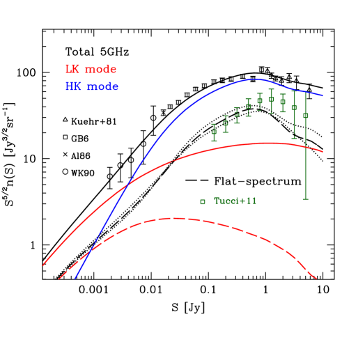
For the model determination we employ number counts at 1.4 and 4.8 GHz. These are mainly based on the NVSS at 1.4 GHz, and on the Northern Green Bank GB6 survey (Gregory et al. 1996) and Kuehr et al. (1981) at 4.8 GHz. We use number counts only for flux densities $S\geq 1$ mJy. At sub-mJy flux densities the relative number of star-forming galaxies and radio-quiet AGN becomes increasingly important (see e.g. Massardi et al. 2010, and references therein). We do not include number counts at frequencies larger than 5 GHz or smaller than 1.4 GHz. The assumption of a single-slope power law spectrum for the core or lobe AGN emission can be considered valid only in a small range of frequencies (see discussion in Sect. 4.5).

Finally, we include in the analysis the estimates of number counts for flat-spectrum sources at 4.8 GHz from Tucci et al. (2011), obtained by combining different surveys between 1.4 and 20 GHz, by extrapolating the spectral energy distribution of flat-spectrum radio sources as discussed in that paper.

As already stated above, for AGN in the LK mode we adopt the FP correlation coefficients provided by Merloni & Heinz (2008): $\xi_{X}=0.62$, $\xi_{M}=0.55$ and $\beta_{R}=8.6$, with an intrinsic scatter of 0.6 dex. We also assume that all LK mode AGN are radio-loud (i.e. $f_{loud}^{LK}=1$). The presence of jets is commonly associated with this class of objects (Merloni & Heinz 2008), in analogy with the low, hard state of black hole X-ray binaries in which radio emission is always detected.

The only free parameters for this AGN population are the coefficients $\xi_{W}$, $\beta_{W}$, and $\sigma_{W}$ of Eqs. 10 and 11 that connect the intrinsic core luminosity to the extended emission from jets and lobes. It is important to keep in mind that these parameters are independent of redshift, and that the time evolution of the LF for LK mode AGN is fully regulated by the evolution of the SMBH mass function and accretion rate (see Sections 2.2 and 2.4).

In order to prevent a too large number of very bright sources, we impose an exponential cut-off in the values of the intrinsic scatter $\sigma_{FP}$ and $\sigma_{W}$ (see Eq. 4 and 11) at high intrinsic core luminosities, with a minimum value of 0.2:

$$\sigma_{FP}=\left\{\begin{array}[]{ll}\sigma_{FP}&\log\mathcal{L}_{c}\leq 34.6\\ \max(\sigma_{FP}\exp(34.6-\log\mathcal{L}_{c}),0.2)&\log\mathcal{L}_{c}>34.6\,.\end{array}\right.$$

$$\sigma_{W}=\left\{\begin{array}[]{ll}\sigma_{W}&\log\mathcal{L}_{c}\leq 31.8\\ \max(\sigma_{W}\exp(31.8-\log\mathcal{L}_{c}),0.2)&\log\mathcal{L}_{c}>31.8\,.\end{array}\right.$$

(24)

The cut-offs on $\sigma_{FP}$ and $\sigma_{W}$ have an impact on luminosity functions only at $L\ga 10^{36}$ and $10^{34}$ erg s^-1 Hz^-1, respectively, and on number counts at the jansky level. We apply the same cut-offs also to HK mode AGN.

We use a Markov chain Monte Carlo (MCMC) method to determine the three model parameters by fitting the BH12-based local LF for low-excitation AGN and the local LF for flat-spectrum sources in the luminosity range dominated by LK mode AGN (i.e. $L\la 10^{30}$ erg s^-1 Hz^-1). We find a very tight linear relation between $\xi_{W}$ and $\beta_{W}$ (see Fig. 4), meaning that only one of them is a real free parameter of the model, with $\xi_{W}$ ranging from 1.3 to 1.45 and $\beta_{W}$ from $-15$ to $-8$. We therefore directly determine $\xi_{w}$ from $\beta_{W}$, using the linear relation displayed in Fig. 4 and Table 3.

The fit is then repeated using $\beta_{W}$ and $\sigma_{W}$ as the only free parameters. In Fig. 5 we show the probability density function (PDF) of the two parameters. We find a significant correlation between the two parameters. The best-fit model is obtained for $\beta_{W}=-12.3$ and $\sigma_{W}=0.94$, while the median values (plus the 68% confidence levels) of the marginalized PDFs are $\beta_{W}=-12.83^{+2.06}_{-1.52}$ and $\sigma_{W}=0.91\pm 0.15$.

As shown in Fig. 5, the model parameters can be in a large range of values, preserving an almost equivalent ability to fit the data. Changing the parameters at the 1$\sigma$ or 2$\sigma$ level around the median has little impact on the LK mode local LF. Differences are more relevant for number counts, as shown in Appendix A. Therefore, we tested the impact of different LK mode models when HK mode AGN are also included and total LFs and number counts are fitted. We consider, in particular, five sets of parameters (shown as large points in Fig. 5): the set that provides the best results will be adopted as our reference model for LK mode AGN in the following analysis. This corresponds to $\{\xi_{w},\,\beta_{w},\,\sigma_{W}\}=\{1.42,\,-13.95,\,0.81\}$ (see Appendix A and the red point in Fig. 5).

As shown in Fig. 6, the model is able to provide a very good fit to the local luminosity function, even for flat-spectrum sources (see also Fig.11). We also compare our predictions with observational estimates of the LK mode LF at $0.5<z<1$ from Best et al. (2014), finding again a good match.

In order to check the hypothesis of $f_{loud}^{LK}=1$, we also included the fraction of radio-loud LK mode AGN among the free parameters. We do not find any significant improvement in the fit and a large fraction of radio-loud AGN ($f_{loud}^{LK}\ga 0.3$) is required from the data.

Using Eq. 12 we can compute the LF associated with the extended jet–lobe AGN emission, starting from the intrinsic core LF (Fig. 7). With respect to the core LF, the peak of the extended jet–lobe LF is shifted to fainter luminosities by around two orders of magnitude. Nevertheless, at high luminosities, the space density for this LF is larger than that associated with the intrinsic core emission and close to the beamed value, as an effect of the large dispersion in the intrinsic core-extended jet–lobe luminosity relation.

The number of free parameters for AGN in the HK mode increases substantially. First of all, the FP relation is not as well established as for LK mode AGN, although there are indications that a correlation is still present for this population of sources. We assume that this relation (Eq. 1) is still valid for HK mode AGN but with unknown coefficients. We impose the continuity condition at $\lambda_{cr}=0.01$ and, as shown in Eq. 3, the only free parameter is $\xi_{X}$. The dispersion in the FP relation is fixed to 0.6, as for LK mode AGN. Other free parameters are the coefficients of the relation between extended and core luminosity (Eq. 10), $\xi_{W}$ and $\beta_{W}$, plus the scatter in the relation, $\sigma_{W}$. Finally, differently from LK mode AGN, the fraction $f_{loud}^{HK}$ of high-accreting SMBHs that are radio-loud (i.e. in the HK mode) is quite uncertain and probably redshift dependent. We parametrize this fraction as a function of redshift as

$$f_{loud}^{HK}(z)=f_{0}(1+z)^{\alpha_{z}}\,,$$

(25)

where $f_{0}$ is the fraction of HK mode AGN at redshift zero. Both $f_{0}$ and $\alpha_{z}$ are free parameters of the model. We impose the condition that $f_{loud}^{HK}(z)\leq 0.3$ at $z=[0,4]$, in agreement with estimates from the literature (Rafter et al. 2009; Kratzer & Richards 2015; Kellermann et al. 2016).

To summarize, we end up with six free parameters ($\xi_{X}$, $\xi_{W}$, $\beta_{W}$, $\sigma_{W}$, $f_{0}$, and $\alpha_{z}$). They can be determined thanks to the wide and composite amount of data to be fitted. Given the LFs and number counts of LK mode AGN, we can compare model predictions with the local LF for the total population of radio-loud AGN and for HK mode AGN⁷⁷7Unless expressly stated otherwise, in the following subsections we are considering the BH12-based data set for the local LFs.; the LF for flat-spectrum sources at $z\simeq 0.3$ and $L\ga 10^{32}$ erg s^-1 Hz^-1; the LF for radio-loud AGN at redshift $z\simeq 0.55$; differential number counts at 1.4 and 5 GHz (at $S\geq 1$ mJy); and differential number counts of flat-spectrum sources at 5 GHz.

Roughly speaking, redshift-independent parameters from FP and core-extended luminosity relations determine the shape of LFs at different redshifts, the shape and the ratio of number counts at 1–5 GHz, while their normalizations are fixed mainly by the fraction of HK mode AGN.

As before, we use a MCMC method to compute the best-fit parameters of the model and to estimate model uncertainties. Some caveats should be taken into account. Firstly, as already seen for LK mode AGN, the parameters show a large degeneracy and correlation with each other. Consequently, the likelihood of the model parameters presents not a single minimum but multiple local minima with comparable values of $\chi^{2}$. Moreover, predicted LFs and number counts are very sensitive to small variations in the model parameters. For example, results are sensitive to variations of $\xi_{W}$ and $\beta_{W}$ lower than 1%, and to variations of $\sigma_{W}$ and $\xi_{X}$ of the order of few per cent. The MCMC inizialization cannot be chosen randomly, but the input parameter set has to be firstly tuned, especially for strongly correlated parameters, otherwise the MCMC algorithm will not be able to converge to a minimum.

As a starting point, we tried to reduce the number of free parameters looking for very tight linear correlations between parameters, as was done for LK mode AGN. We proceeded in the following way. We ran the MCMC algorithm with different input parameter sets, covering a large range of possible values for the input parameters. We find that MCMC chains converge to local minima that depend on the inizialization of parameters. A strong linear relation is found between $\xi_{w}$ and $\beta_{W}$ (see Fig. 8), similarly to LK mode AGN. The correlation is valid over a very large range of values for $\beta_{W}$, from 0 to 10. We decided therefore to fix the parameter $\xi_{w}$ using the linear fit displayed in Fig. 8 and Table 3.

The MCMC method was then run again with the remaining parameters. The results are now less sensitive to the initialization and the algorithm is able to converge to the global minimum starting from any reasonable parameter set. In Fig. 9 we show the marginalized PDFs of the parameters, while in Table 3 we report the best-fit model, the median, and the uncertainties of the parameters, and in Table 4 the $\chi^{2}$ of the fit to the different data sets. We still find a significant correlation among the parameters, and in particular between $\xi_{X}$, $\beta_{W}$, and $f_{0}$. The power-law index $\xi_{W}$ is found between 0.6 and 0.95, very close to the theoretical expectation of 0.8 (see discussion in Sect. 2.4), while the parameter $\beta_{W}$ covers a large range of values, between 2 and 14. This means that the normalization coefficient in the core and extended luminosity relation can vary by more than ten orders of magnitude. It is interesting to compare this result with the range of values for LK mode AGN: [$-8,\,-16$]. AGN in LK and HK mode therefore have quite a different relationship between core and extended luminosity: using the best-fit models, for an intrinsic core luminosity of $\log\mathcal{L}_{c}=27\,(30)\,[33]$ (in erg s^-1 Hz^-1) we get $\log L_{ex}=28.8\,(31.1)\,[33.5]$ for HK mode AGN and $24.4\,(28.6)\,[32.9]$ for LK mode AGN. We conclude therefore that the model typically predicts a much stronger contribution of extended jets and lobes for the former AGN class.

The FP parameter $\xi_{X}$ is found between 1.5 and 1.9, about three times larger than the value used for LK mode AGN, and (unlike LK mode AGN) the intrinsic core luminosity is anti-correlated with the SMBH mass. These results are in good agreement with observational constraints of the FP relation for high-accretion AGN (Dong et al. 2014).

The fraction of HK mode AGN is between 0.5 and 1 per mil at $z\simeq 0$, and it steeply increases with redshift, with $\alpha_{z}$ ranging from 1.8 to 2.4 (increasing $f_{0}$, $\alpha_{z}$ decreases). Models predict therefore a very low fraction of high-accreting AGN in the HK mode, especially in the local Universe, with $f_{loud}^{HK}\ll 1$ per cent at $z=0$–1, between 0.4–1 per cent at $z\simeq 2$ and 1–2.4 per cent at $z\simeq 4$ (see Fig. 10).

Figures 11 and 13 provide a visual check of the model fits to observational data, and in particular to the fits used in the parameters determination (corresponding to the BH12-based data set for the local LFs). In these figures, along with the best-fit model, we also consider lower and upper limit cases that should provide a rough estimate of uncertainties in model predictions. As the upper limit we take a model with $f_{0}\simeq 0.14$%, $\xi_{X}\simeq 1.5$, and $\beta_{W}\simeq 3$, while as the lower limit a model with $f_{0}\simeq 0.03$%, $\xi_{X}\simeq 1.9$, and $\beta_{W}\simeq 16$.

In Fig. 11 we consider the local LF at 1.4 GHz for the total population of radio-loud AGN and for HK mode AGN. The former is quite well reproduced by the model in the whole luminosity range in which data are available.

It is more interesting to focus on HK mode AGN. The best-fit model provides a good fit to the BH12 HK mode space densities at $L\ga 10^{30}$ erg s^-1Hz^-1, whereas it tends to underestimate BH12 estimates at lower luminosities. A better agreement is found for models that predict a relatively large local fraction of HK mode AGN ($f_{0}\approx 0.1$%). Model predictions of the HK mode local LF always show a maximum at $L>10^{29}$ erg s^-1Hz^-1 and a decrease at lower luminosities. On the contrary, BH12 measurements seem to keep increasing while moving to low luminosities (we recall that the first points in the BH12 HK mode LF should be considered as lower limits).

The local LF for flat-spectrum sources is also consistent with observational data (Toffolatti et al. 1987; Padovani et al. 2007) over the seven orders of magnitudes covered by them. It is interesting to note how model predictions for the local LF of flat-spectrum HK mode sources can vary at low to intermediate luminosities according to the parameter set used. At $\approx 10^{29}$ erg s^-1Hz^-1, the upper and lower cases differ by about two orders of magnitude. This is due to the dependence of the extended jet–lobe LF on the $\xi_{W}$ (or $\beta_{W}$) parameter. As shown in Fig. 12, changing the value of $\xi_{W}$ from 0.78 to 1.25, the peak of the LF moves from $10^{30}$ to $10^{27}$ erg s^-1Hz^-1. With low values of $\xi_{W}$, therefore, extended emission from jets and lobes is typically fainter and the number of flat-spectrum sources increases.

Finally, models provide a very good fit to number counts of the AGN population at 1.4 GHz and at 5 GHz, and of the flat-spectrum sources at 5 GHz, as shown in Fig. 13. Number counts are dominated by AGN in HK mode starting from flux densities $\ga 10$ mJy. There are no relevant differences among model predictions using different parameter sets, mainly due to the strong constraints imposed by number counts at 1.4 GHz at $S\la 0.1$ Jy. Some scatter is observed, but only at the jansky level for flat-spectrum sources.

Smolčić et al. (2017a) provided separate estimates of number counts for low- to moderate-luminosity AGN (analogous to LK mode) and moderate- to high-luminosity AGN (mostly analogous to HK mode). Very remarkably, although these data are not considered for the fit, the agreement between these number counts and the predictions of our current models is excellent (as displayed in the left panel of Fig. 13).

Model parameters are also determined using the P16-based data set (see Table 3). With respect to the BH12-based one, the main change is the much higher fraction of HK mode AGN found at low to intermediate luminosities in the local LF. The P16 and BH12 measurements of the LK mode and total local LF are instead consistent with each other, at least for $L\ga 10^{30}$ erg s^-1Hz^-1 (see Fig 3).

For LK mode AGN, the model predicts a quite similar local LF at intermediate to high luminosities, indepedent of the data set, with some differences only at low luminosities ($L<10^{29}$ erg s^-1Hz^-1). In terms of parameters, $\beta_{W}$ from the P16 data set is about 20 per cent smaller with respect to the BH12-based case.

The impact of the different HK mode local LF is quite significant on the model. As expected, the most affected parameter is the local fraction of HK mode AGN, whose best-fit value is now about five times the BH12-based one (i.e. $f_{0}\sim 3$ per mil). The evolution of the HK mode fraction is softer than before, as shown in Fig. 10, and compatible with previous results at high redshifts. The best-fit values for the parameters $\beta_{w}$ and $\xi_{X}$ are smaller than the BH12-based results, especially $\beta_{W}$, but still compatible with them at the 2$\sigma$ level. The predicted number counts are instead very similar to the BH12-based ones due to the strong constraints imposed by observational data. The larger $\chi^{2}$ found for the P16-based best-fit model is mainly due to the poor fit to the HK mode local LF (see Table 4).