Modeling the impact of birth control policies on China’s population and age: effects of delayed births and minimum birth age constraints

Now, in order to introduce a delay between consecutive births, we need to further partition the female population into those who have never had a child and those who have already had a child (and who may need to wait a certain time before having another one). The population densities for each of these classes of females are defined as:

$f_{0}(t,a)$:

the population density of childless females. The quantity $f_{0}(t,a)\textrm{d}a$ is the number of females with age between $a$ and $a+\textrm{d}a$ and who have never had a child up to the current time $t$.

$f(t,a,\tau)$:

the population of females who have had at least one child. The quantity $f(t,a,\tau)\textrm{d}a\textrm{d}\tau$ is the number of females at time $t$ whose age is between $a$ and $a+\textrm{d}a$ and whose youngest child’s age is between $\tau$ and $\tau+\textrm{d}\tau$.

We will assume that these two populations have the same age-dependent death rate $\mu_{\rm f}(a)$ but give birth at different rates $\beta_{0}(a)$ and $\beta(a,\tau)$, respectively. We also define the total female population density as

$$f_{\rm tot}(t,a)=f_{0}(t,a)+\int_{0}^{a}\!f(t,a,\tau)\textrm{d}\tau$$

(2)

and the total number of females at time $t$ as

$$n(t)=\int_{0}^{\infty}\!\!f_{\rm tot}(t,a)\textrm{d}a=\int_{0}^{\infty}\!\!f_{0}(t,a)\textrm{d}a+\int_{0}^{\infty}\!\!\textrm{d}a\int_{0}^{a}\!\!\textrm{d}\tau f(t,a,\tau).$$

(3)

The age-structured McKendrick equations for $f_{0}$ and $f$ are:

	$\displaystyle\frac{\partial}{\partial t}f_{0}(t,a)+\frac{\partial}{\partial a}f_{0}(t,a)$	$\displaystyle={}-\left(\mu_{\rm f}(a)+\beta_{0}(a)\right)f_{0}(t,a)$		(4a)
	$\displaystyle\frac{\partial}{\partial t}f(t,a,\tau)+\frac{\partial}{\partial a}f(t,a,\tau)+\frac{\partial}{\partial\tau}f(t,a,\tau)$	$\displaystyle={}-\left(\mu_{\rm f}(a)+\beta(a,\tau)\right)f(t,a,\tau)$		(4b)
	$\displaystyle f_{0}(t,0)$	$\displaystyle=\eta\left(\int_{0}^{\infty}\!\!\beta_{0}(a)f_{0}(t,a)\textrm{d}a+\int_{0}^{\infty}\!\!\textrm{d}a\int_{0}^{a}\!\!\textrm{d}\tau\,\beta(a,\tau)f(t,a,\tau)\right)$		(4c)
	$\displaystyle f(t,a,0)$	$\displaystyle=\beta_{0}(a)f_{0}(t,a)+\int_{0}^{a}\!\!\beta(a,\tau)f(t,a,\tau)\textrm{d}\tau$		(4d)
	$\displaystyle f_{0}(0,a)$	$\displaystyle=I_{0}(a)\quad\text{and}\quad f(0,a,\tau)=I(a,\tau).$		(4e)

Equation (4a) describes the evolution of $f_{0}$ as in the classical McKendrick equation (cf Eq. (1a)) with birth rate $\beta_{0}(a)$. For $f(t,a,\tau)$, we must introduce the new variable $\tau$ to mark the time since the last birth. This brings in another convection term in Eq. (4b) since $\tau$ increases alongside time $t$ and age $a$. The birth rate $\beta$ for this population can depend on both the age $a$ and the time $\tau$ since the last birth. Eq. (4c) gives the number of girls $f_{0}(t,0)$ born at time $t$, while Eq. (4d) describes $f(t,a,0)$, the density of females at age $a$ at time $t$ who just gave birth. These individuals can arise from the $f_{0}$ population (females who have never had a child) or from the $f$ population itself (females who have already had at least one child). Thus, the boundary conditions  (4c) and  (4d) couple the two populations $f_{0}$ and $f$. Finally, equations (4e) simply describe the initial conditions for $f_{0}$ and $f$.

In Appendix A, we explicitly show that the total female population density $f_{\rm tot}(t,a)$ (Eq. (2)) satisfies the standard age-structured McKendrick equation

$$\begin{split}\frac{\partial}{\partial t}f_{\rm tot}(t,a)+\frac{\partial}{\partial a}f_{\rm tot}(t,a)=-\mu_{\rm f}(a)f_{\rm tot}(t,a).\end{split}$$

(5)

Within a model that explicitly considers the time $\tau$ since the last childbirth, we can easily describe an imposed hypothetical policy that applies a refractory period $\delta$ between births. After having a child and before this refractory period ($0\leq\tau\leq\delta$) expires, the birth rate $\beta(a,\tau)$ can be set to $0$. As a preliminary description, we will consider a policy-modified (truncated) birth rate function

$$\beta(a,\tau)=\beta_{0}(a)\mathds{1}(\tau,\delta)$$

(6)

where the indicator function $\mathds{1}(\tau,\delta)=1$ for $\tau>\delta$ and $\mathds{1}(\tau,\delta)=0$ for $\tau\leq\delta$. This form assumes that once the imposed refractory period has past, the birth rate immediately rises back to a value associated with the persons current age.

We first analyze the asymptotic behavior of our model. An important feature of renewal transport equations such as the McKendrick model is that as $t\to\infty$, the total population $n(t)$ will grow exponentially (in the absence of nonlinear regulation terms (Gurtin and MacCamy, 1974)), while the normalized, age-dependent population density converges to a time-independent stationary distribution (see Perthame (2007, Chapter 3) and Arino (1995)). This property is independent of the initial condition. We will assume that this steady-state asymptotic property arises in our two-component, three-variable model; i.e., the normalized densities $f_{0}(t,a)/n(t)$ and $f(t,a,\tau)/n(t)$ converge to stationary distributions. We denote the stationary limits as

$$\lim_{t\to\infty}\frac{f_{0}(t,a)}{n(t)}\equiv h_{0}(a)\quad\text{and}\quad\lim_{t\to\infty}\frac{f(t,a,\tau)}{n(t)}\equiv h(a,\tau).$$

(7)

We also define the distribution associated with the total female population as

$$\lim_{t\to\infty}\frac{f_{\rm tot}(t,a)}{n(t)}\equiv h_{\rm tot}(a)=h_{0}(a)+\int_{0}^{a}\!h(a,\tau)\textrm{d}\tau,$$

(8)

where $\int_{0}^{\infty}h_{\rm tot}(a)\textrm{d}a=1$. If we assume that $f_{0}(0,a)/n(0)=h_{0}(a)$ and $f(0,a,\tau)/n(0)=h(a,\tau)$ for any $a,\tau$ at some initial time $t=0$, then $f_{0}(t,a)/n(t)=h_{0}(a)$ and $f(t,a,\tau)/n(t)=h(a,\tau)$ hold for any $t\geq 0$.

From Eq. (4a), we have

	$\displaystyle\frac{1}{f_{0}(t,a)}\frac{\partial f_{0}(t,a)}{\partial t}$	$\displaystyle=-\frac{1}{f_{0}(t,a)}\frac{\partial f_{0}(t,a)}{\partial a}-\mu_{\rm f}(a)$		(9)
		$\displaystyle=-\frac{n(t)}{f_{0}(t,a)}\frac{1}{n(t)}\frac{\partial f_{0}(t,a)}{\partial a}-\mu_{\rm f}(a)$
		$\displaystyle=\frac{1}{h_{0}(a)}\frac{\textrm{d}h_{0}(a)}{\textrm{d}a}-\mu_{\rm f}(a).$

Thus, $[\partial f_{0}(t,a)/\partial t]/f_{0}(t,a)$ is independent of $t$. Moreover, for any $a,a^{\prime},\tau$

$$\frac{f_{0}(t,a)}{f(t,a^{\prime},\tau)}=\frac{h_{0}(a)}{n(t)}\frac{n(t)}{h(a^{\prime},\tau)}=\frac{h_{0}(a)}{h(a^{\prime},\tau)}$$

(10)

is also independent of $t$ so that

$$\frac{\partial}{\partial t}\left[\frac{f_{0}(t,a)}{f(t,a^{\prime},\tau)}\right]=\frac{1}{f(t,a^{\prime},\tau)^{2}}\left[f(t,a^{\prime},\tau)\frac{\partial}{\partial t}f_{0}(t,a)-f_{0}(t,a)\frac{\partial}{\partial t}f(t,a^{\prime},\tau)\right]=0.$$

(11)

Thus, for any $a,a^{\prime},\tau$,

$$\frac{1}{f_{0}(t,a)}\frac{\partial f_{0}(t,a)}{\partial t}=\frac{1}{f(t,a^{\prime},\tau)}\frac{\partial f(t,a^{\prime},\tau)}{\partial t}=\frac{1}{f_{0}(t,a^{\prime})}\frac{\partial f_{0}(t,a^{\prime})}{\partial t}.$$

(12)

Eqs. (9) and (12) show that $[\partial f_{0}(t,a)/\partial t]/f_{0}(t,a)$ is independent of both $t$ and $a$, allowing us to define a constant that describes the stationary growth rate

$$\lambda=\frac{1}{f_{0}(t,a)}\frac{\partial f_{0}(t,a)}{\partial t}=\frac{1}{f(t,a,\tau)}\frac{\partial f(t,a,\tau)}{\partial t}=\frac{1}{f_{\rm tot}(t,a)}\frac{\partial f_{\rm tot}(t,a)}{\partial t}.$$

(13)

Thus, we can express solutions for the densities $f_{0}(t,a)$ and $f(t,a,\tau)$ in the form

$$f_{0}(t,a)=Ch_{0}(a)e^{\lambda t}\quad\text{and}\quad f(t,a,\tau)=Ch(a,\tau)e^{\lambda t},$$

(14)

where $C$ is a constant. After using these expressions in Eqs. (4), we find the equations for the stationary distributions

	$\displaystyle\frac{\textrm{d}}{\textrm{d}a}h_{0}(a)$	$\displaystyle=-\left(\mu_{\rm f}(a)+\beta_{0}(a)+\lambda\right)h_{0}(a)$		(15a)
	$\displaystyle\frac{\partial}{\partial a}h(a,\tau)+\frac{\partial}{\partial\tau}h(a,\tau)$	$\displaystyle=-\left(\mu_{\rm f}(a)+\beta(a,\tau)+\lambda\right)h(a,\tau)$		(15b)
	$\displaystyle h_{0}(0)$	$\displaystyle=\eta\left(\int_{0}^{\infty}\beta_{0}(a)h_{0}(a)\textrm{d}a+\int_{0}^{\infty}\!\!\textrm{d}a\int_{0}^{a}\!\textrm{d}\tau\,\beta(a,\tau)h(a,\tau)\right)$		(15c)
	$\displaystyle h(a,0)$	$\displaystyle=\beta_{0}(a)h_{0}(a)+\int_{0}^{a}\!\beta(a,\tau)h(a,\tau)\textrm{d}\tau.$		(15d)

Next, using Eq. (5), we find

$$\frac{\textrm{d}}{\textrm{d}a}h_{\rm tot}(a)=-\left(\mu_{\rm f}(a)+\lambda\right)h_{\rm tot}(a),$$

(16)

which is solved by

$$h_{\rm tot}(a)=h_{\rm tot}(0)\exp\left[-a\lambda-\int_{0}^{a}\!\!\mu_{\rm f}(a^{\prime})\textrm{d}a^{\prime}\right].$$

(17)

We can then define the effective whole-population birth rate function

$$\beta_{\rm eff}(a)=\frac{\beta_{0}(a)h_{0}(a)+\int_{0}^{a}\!\beta(a,\tau)h(a,\tau)\textrm{d}\tau}{h_{\rm tot}(a)},$$

(18)

which describes the overall birthrate weighted over the entire stationary population. This population-averaged birth rate $\beta_{\rm eff}(a)$ corresponds to that used in the basic lumped model (Eq. (1b)) and is the quantity that can be directly extracted from birth data that provide women’s ages at time of birth, but that may not distinguish whether females are first-time mothers. We prove in Appendix B that given $\beta_{\text{eff}}(a)$, the new-mother birth rate function can be calculated from

$$\beta_{0}(a)=\frac{\beta_{\text{eff}}(a)}{1-\int_{0}^{\delta}\beta_{\text{eff}}(a-\tau)\textrm{d}\tau},$$

(19)

which then allows us to reconstruct $\beta(a,\tau)$ from Eq. (6). Using $\beta_{\rm eff}$, the boundary condition for Eq. (16), the counterpart to Eq. (15c), can be written as

$$h_{\rm tot}(0)=\eta\int_{0}^{\infty}\beta_{\rm eff}(a)h_{\rm tot}(a)\textrm{d}a.$$

(20)

Finally, after using the solution in Eq. 17 for $h_{\rm tot}(a)$ in Eq. (20), we find an equation for $\lambda$:

$$z(\lambda)\equiv\eta\int_{0}^{\infty}\beta_{\rm eff}(a)\exp\left[-a\lambda-\int_{0}^{a}\mu_{\rm f}(a^{\prime})\textrm{d}a^{\prime}\right]\textrm{d}a=1.$$

(21)

The function $z(\lambda)$ is monotonically decreasing with $\lambda$ and obeys the limits $\lim_{\lambda\to+\infty}z(\lambda)=0$ and $\lim_{\lambda\to-\infty}z(\lambda)=+\infty$. Thus, Eq. (21) has a unique solution that can easily be found numerically. From Eq. (21), the solution for $\lambda$–the net population growth rate–clearly increases with $\beta_{\rm eff}(a)$ and decreases with $\mu_{\rm f}(a)$.

With $\beta_{0}(a)$ and $\lambda$ determined by Eqs.  (19) and (21), respectively, we can explicitly find $h(a,\tau)$. First, we use the normalization condition $\int_{0}^{\infty}h_{\rm tot}(a)\textrm{d}a=1$ on Eq. (16) to explicitly find $h_{\rm tot}(0)$ in terms of $\lambda$ and $\mu_{\rm f}(a)$. Since $h(0,\tau)=0$, we have $h_{0}(0)=h_{\rm tot}(0)$, which allows us to explicitly express the solution to Eq. (15a):

$$h_{0}(a)=h_{0}(0)\exp\left[-a\lambda-\int_{0}^{a}\big{(}\mu_{\rm f}(a^{\prime})+\beta_{0}(a^{\prime})\big{)}\textrm{d}a^{\prime}\right].$$

(22)

Next, we use Eq. (15d) and Eq. (18) to eliminate $\beta(a,\tau)$ and find $h(a,0)=h_{\rm tot}(a)\beta_{\text{eff}}(a)$, which is known. Thus, we can explicitly calculate $h(a,\tau)$ by solving Eq. (15b) using the method of characteristics:

$$h(a,\tau)=h(a-\tau,0)\exp\left[-\tau\lambda-\int_{a-\tau}^{a}\big{(}\mu_{\rm f}(a^{\prime})+\beta(a^{\prime},a^{\prime}-a+\tau)\big{)}\textrm{d}a^{\prime}\right].$$

(23)

To summarize, starting from $\beta_{\text{eff}}(a),\mu_{\rm f}(a),\eta$ (measured, say), and $\delta$, we can compute the growth rate $\lambda$ numerically, then analytically reconstruct $\beta_{0}(a),\beta(a,\tau),h_{0}(a)$ and $h(a,\tau)$.

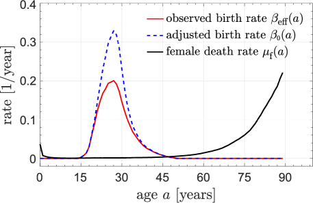
We now use the Chinese national census data recorded in 1982 (Population Census Office under the State Council, 1985) to infer the overall birth rate $\beta_{\rm eff}(a)$ and the female death rate $\mu_{\rm f}(a)$ functions in China in 1981. Although gestation imposes a hard refractory period of $\delta\approx 9$ months, some time is needed to recover from childbirth and the birth rate should more gradually recover. Specifically, in 1981 China, extended breastfeeding was common, which prevents the next pregnancy (Xu et al., 2009). Thus, we will assume the birth rate returns to normal approximately only after about two years. Therefore, when there is no policy that controls the interval between births, we set $\delta=2$ years such that $\beta(a,\tau)=0$ for $\tau<2$ years and $\beta(a,\tau)=\beta_{0}(a)$ for $\tau>2$ years. For other societies, this natural refractory period might be shorter. Using $\delta=2$ and Eq. (19), we calculate $\beta_{0}(a)$ from $\beta_{\text{eff}}(a)$ derived from data. These rates are illustrated in Fig. 1. Note that $\beta_{0}(a)$ for 1981 has already been mildly affected by the incipient birth-control policies in China.

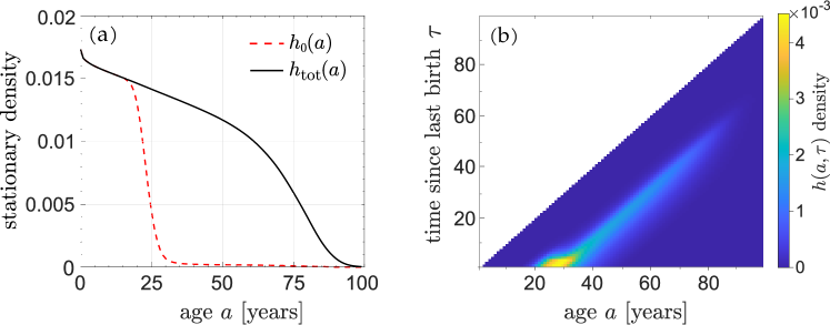
Using the birth rate $\beta_{\rm eff}(a)$ and death rate $\mu_{\rm f}(a)$ shown in Fig.  1, we solve Eqs. (15) to find $h_{0}(a)$ and $h(a,\tau)$, and plot them with $h_{\rm tot}(a)$ given by Eq. (17) in Fig. 2(a,b).

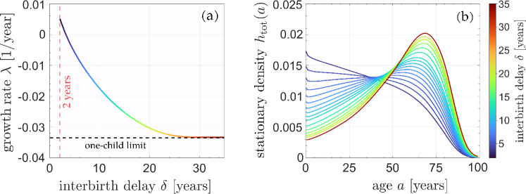
To explore the effects of an imposed refractory period, we first set $\delta=2$ years, apply the newborn sex ratio of China in 1981, $\eta=0.48$, and solve Eq. (21). We find $\lambda\simeq 0.005>0$, indicating an exponentially growing total population. This stationary growth rate is much smaller than the actual growth rate of China in 1981, which is 0.0146. One reason is that in 1981, the proportion of younger females is much higher than that in the stationary distribution $h_{\rm tot}$. The shape of $h_{\rm tot}(a)$ is consistent with this growth as it is monotonically decreasing, indicating that every new generation has a larger population than the previous one. In Fig. 3, we see how increases in the refractory period $\delta$ decrease the asymptotic growth rate $\lambda$ and affect the distribution $h_{\rm tot}(a)$. A negative overall birth rate $\lambda<0$ (i.e., an asymptotically decaying population) arises when $\delta\gtrsim 3.22$ years $\approx 39$ months. As soon as $\lambda<0$, the distribution $h_{\rm tot}(a)$ becomes nonmonotonic, and a peak in the female population distribution arises at a finite age $a>0$.

If $\delta$ is set sufficiently large, a female cannot have a second child, and the outcome is equivalent to a strict one-child policy. We use the terminology “strict one-child policy” for the scenario in which each female can have strictly no more than one child, while we use “one-child policy” to refer to the actual policy realized in practice. From 1980 to 1990, the one-child policy contained many exceptions, allowing one to bear more than one child (Nie, 1999).

Our formulation is valid only in the asymptotic case with a fixed delay $\delta$ that remains unchanged for a long period of time. For practical modeling of policies in which delays $\delta$ are used as a time-dependent control variable, such as China’s 1980 one-child policy and its subsequent modification in 2015, it is necessary to analyze the full model that delineates the two female populations.

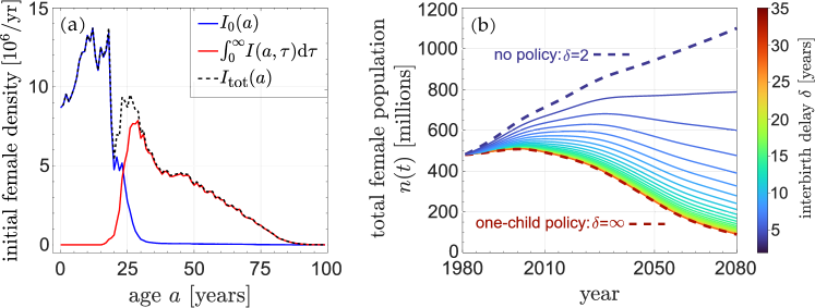
As was used to predict the effects of the one-child policy, we use China’s female age distribution in 1981 (Population Census Office under the State Council, 1985) as a starting point to explore how the total population evolves under different values of the imposed delay $\delta$. Since the data only contain total female numbers $I_{\rm tot}(a)$ and not $I_{0}(a)$ and $I(a,\tau)$ individually, we use $I_{0}(a)=I_{\rm tot}(a)h_{0}(a)/h_{\rm tot}(a)$ and $I(a,\tau)=I_{\rm tot}(a)h(a,\tau)/h_{\rm tot}(a)$ to reconstruct these initial age distributions. These initial distributions are plotted in Fig. 4(a). With these initial conditions, we can solve Eq. (4a) and Eq. (4b) with the method of characteristics to find the full age and time dependence of the female populations

	$\displaystyle f_{0}(t,a)$	$\displaystyle=f_{0}(t-a,0)\exp\left[-\int_{0}^{a}\!\big{(}\mu_{\rm f}(a^{\prime})+\beta_{0}(a^{\prime})\big{)}\textrm{d}a^{\prime}\right]\ \text{if }t>a$		(24a)
	$\displaystyle f_{0}(t,a)$	$\displaystyle=I_{0}(a-t)\exp\left[-\int_{a-t}^{a}\!\big{(}\mu_{\rm f}(a^{\prime})+\beta_{0}(a^{\prime})\big{)}\textrm{d}a^{\prime}\right]\ \ \ \text{if }t\leq a,$		(24b)

	$\displaystyle f(t,a,\tau)$	$\displaystyle=f(t-\tau,a-\tau,0)\exp\left[-\int_{a-\tau}^{a}\!\big{(}\mu_{\rm f}(a^{\prime})+\beta\left(a^{\prime},a^{\prime}-(a-\tau)\right)\big{)}\textrm{d}a^{\prime}\right]\ \text{if }t>\tau$		(25a)
	$\displaystyle f(t,a,\tau)$	$\displaystyle=I(a-t,\tau-t)\exp\left[-\int_{a-t}^{a}\!\big{(}\mu_{\rm f}(a^{\prime})+\beta\left(a^{\prime},a^{\prime}-(a-\tau)\right)\big{)}\textrm{d}a^{\prime}\right]\ \ \ \ \ \ \text{if }t\leq\tau.$		(25b)

Females are fertile only between sexual maturity and menopause. Thus, we set $a_{\min}$ ($\sim 12$ years) and $a_{\max}$ ($\sim 50$ years), so that $\beta_{0}(a)=\beta(a,\tau)=0$ for $a<a_{\min}$ or $a>a_{\max}$. Recall that an imposed policy delayed-birth policy is manifested by $\beta(a,\tau)=0$ for $\tau<\delta$. Eq. (4c) becomes

$$f_{0}(t,0)=\eta\left(\int_{a_{\min}}^{a_{\max}}\!\!\beta_{0}(a)f_{0}(t,a)\textrm{d}a+\int_{a_{\min}}^{a_{\max}}\!\!\!\textrm{d}a\int_{\delta}^{a}\!\!\textrm{d}\tau\,\beta(a,\tau)f(t,a,\tau)\right).$$

(26)

For $t\leq\gamma\equiv\min\{a_{\min},\delta\}$, the $f_{0}(t,a)$ and $f(t,a,\tau)$ terms in the integrands in Eq. (26) can be solved by Eq. (24b) and Eq. (25b). Thus, we can express $f_{0}(t,0)$ in terms of $I_{0}(a),I(a,\tau),\beta_{0}(a),\beta(a,\tau)$, and $\mu_{\rm f}(a)$. Using Eqs. (24), we can calculate $f_{0}(t,a)$ for any $a$ and $t\leq\gamma$. Under the imposed refractory period, Eq. (4d) becomes

$$f(t,a,0)=f_{0}(t,a)\beta_{0}(a)+\int_{\delta}^{a}\!\!\beta(a,\tau)f(t,a,\tau)\textrm{d}\tau.$$

(27)

If $t\leq\gamma$, we can also use Eq. (25b) for $f(t,a,\tau)$ in the integrand of Eq. (27), and then use the solved $f_{0}(t,a)$ to express $f(t,a,0)$ in terms of $I_{0}(a),I(a,\tau),\beta_{0}(a),\beta(a,\tau)$, and $\mu_{\rm f}(a)$. Using Eqs. (25), we can calculate $f(t,a,\tau)$ for any $a,\tau$ and $t\leq\gamma$. Finally, using $f_{0}(\gamma,a),f(\gamma,a,\tau)$ as the initial conditions, we can solve $f_{0}(t,a),f(t,a,\tau)$ for $t\leq 2\gamma$. Repeating this procedure, we can use $I_{0}(a),I(a,\tau),\beta_{0}(a),\beta(a,\tau)$, and $\mu_{\rm f}(a)$ to calculate $f_{0}(t,a)$ and $f(t,a,\tau)$ for any $t,a,\tau$.

Using the fundamental rates $\beta_{0}(a)$, $\mu_{\rm f}(a)$ and $\beta(a,\tau)$ as those used in the previous subsection for the full model (see Fig. 1 and Eq. (6)), we use the above procedure to construct the total female population $n(t)$ (see Eq. 3). The evolution of $n(t)$ over one century, under different interbirth delays, are plotted in Fig. 4(b). At long times, the total population exhibits the asymptotic behavior predicted by the eigenvalues shown in Fig. 3(a). For $\delta\gtrsim 3.22$ years, the total population will decrease exponentially. Because the total population growth rate is most sensitive to small values of imposed delay $\delta$, even a delay of $\delta\sim 4$ years is sufficient to dramatically reduce population over the next $100$ year, compared to the $\delta=2$ case of no refractory period.

The formal results and analyses above can be generalized to include time dependent parameters $\mu_{\rm f}(t,a)$, $\beta_{0}(t,a)$, $\beta(t,a,\tau)$, and even $\delta(t)$ to reflect social and policy changes. In this case, am imposed refractory period would be defined by the time-dependent birth rate function $\beta(t,a,\tau)=\beta_{0}(t,a)\mathds{1}(\tau>\delta(t))$ and the population densities will need to be evaluated numerically.

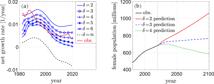
First, we use parameters inferred from 1981 Chinese data in our model to predict population growth for different values of $\delta$. When we compare predicted net growth rates with those derived from 1981-2020 data, shown in Fig. 5(a), we see that (i) during 1981-1990, the observed growth rate is close to that when $\delta=2$¹¹1This means that there was effectively no interbirth period policy and that the the adjusted birth rate $\beta_{0}(a)$ was not changed much during the lax birth-control policies during this period (Li and Wong, 2020).; (ii) from 1991 to 2010, the observed growth rate was close to that predicted from a model with $\delta=5$, possibly due to harsher policies like coerced abortion (Nie, 1999); (iii) after 2011, the observed growth rate rose to a level close to that of a model with $\delta=3\sim 4$, indicating a de facto relaxation of the one-child policy. Indeed, after 2011, policies that encouraged births were initiated. Starting in 2011, a couple was allowed to have up to two children if both parents never had siblings. Then, starting in 2014, a couple can have up to two children if at least one of the parents never had a sibling. Finally, starting in 2016, couples could bear up to two children regardless of their sibling status (Kane and Li, 2021). These policies might explain the flattening and subsequent increase in the net growth rate starting about 2011. However, the effects of these policies might be temporary. After the two-child policy in 2016, the net growth rate increased to the level consistent with a $\delta=3$ model but soon returned to the level closer a $\delta=4$ model. The actual growth rate is higher than in the $\delta=\infty$, strict one-child policy model. This indicates that many couples had, legally or illegally, more than one child.

Starting in 2021, a new policy allows any couple to have up to three children without penalty. We make different predictions for the effect of this three-child policy. The optimistic prediction is that the policy can fully stimulate childbearing to the point that the net growth rate can reach the level predicted by a $\delta=2$ model, but this could be realized only if behavior and cultural-economic changes have not affected an intrinsic propensity for childbearing. Another possibility is that the policy has no significant effect so that the net growth rate will only increase modestly and transiently before effectively reducing back to that consistent with a $\delta=4$ model. See Fig. 5(b) for different predictions of population over the 2021-2100 time frame.

Besides mandating a refractory period between births, another method of population control is to impose a minimum childbearing age. The minimum age $a_{\rm min}$ is thus set by policy rather than by physiology. For example, starting in 1985, in Yicheng county, Shanxi province, a couple could bear two children, but the first child was allowed only after the mother turned 24, and the second child was allowed only after the mother turned 30 (Qin and Wang, 2017).²²2In China, the legal marriage age for females is 20 implying an existing soft constraint of $a_{\rm min}\approx 21$.

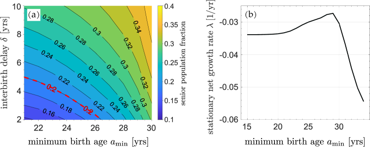
One side-effect of population control is a distribution shifted toward older ages. In China, the percentage of seniors (65+) increased from $5\%$ in 1981 to $13\%$ in 2020 (Man et al., 2021). Policies such as imposing interbirth delays $\delta$ and minimum childbearing ages $a_{\min}$ can both affect the long term senior (65+) population. Fig. 6(a) shows a contour plot of the percentage of seniors as a function of imposed $\delta$ and $a_{\min}$. In order to maintain the senior population under $20\%$ (the red dashed line), the overall policy must not be too drastic. Nonetheless, with two strategies, a balanced combination can be used. For example, one can set $a_{\min}=26,\delta=2$, or $a_{\min}=24,\delta=4$, or $a_{\min}=21,\delta=5$ and still prevent the senior population from exceeding $20\%$ far in the future.

Although increasing the minimum childbearing age $a_{\min}$ should reduce the rate of childbirth, we observe a counter-intuitive scenario in which the net growth rate is nonmonotonic in $a_{\min}$. Under the strict one-child policy (i.e., $\delta=\infty$), increasing $a_{\min}$ will first increase the stationary net growth rate $\lambda$ before decreasing it, as shown in Fig. 6(b). Under a perpetual strict one-child policy, the population in each successive generation is roughly halved and the total number of future newborns is roughly the current population. Although decreasing $a_{\min}$ can temporarily increase the total population, it accelerates the “halving process” in the long run since the interval between successive generations is shorter. When $a_{\min}$ is not large, almost every woman can have one child anyway. Further increasing $a_{\min}$ will decrease $\lambda$ as more women start to be pushed past their childbearing years without giving birth; thus, a maximum in the growth rate $\lambda$ arises at $a_{\min}\approx 29$.

We used $\eta=0.48$, the fraction of female births 1981 China, to generate the results presented in Section 2. Due to subsequent sex-selective abortions biased towards males, the value of $\eta$ dropped to $0.45$ in 2005 before gradually increasing (Zeng et al., 1992; Goodkind, 2011; Li and Meng, 2014).

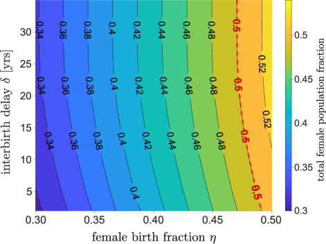
We can alter the value of $\eta$ and calculate the stationary female fraction of total population, which is also affected by the interbirth delay $\delta$. Fig. 7 illustrates the stationary female percentage as a function of $\eta$ and $\delta$. When $\delta=2$, the stationary female percentage is approximately 1% higher than the female percentage $\eta$ at birth. When we fix $\eta$ and increase $\delta$, the stationary female fraction also increases. When $\delta=\infty$, the stationary female population is approximately 3% higher than $\eta$. For larger $\delta$, the stationary age distribution is shifted to larger ages. Since the female death rate $\mu_{\rm f}(a)$ is lower than the male death rate $\mu_{\rm m}(a)$ at larger ages $a$, the female percentage increases with age (in 1981 China, newborns were 48% female while 65+ seniors were 56% female).

We have discussed the policy of applying a refractory period between births and predicted its effects. We assume that the birth rate returns to normal after the refractory period, meaning that people obey this policy and do not respond with compensatory behaviors. In reality, people who want to have more children might mitigate the effects of control policies by, for example, giving birth again immediately after the end of the refractory period following the previous birth. In addition to this “catch up” strategy to recover from the “missed opportunity,” people might also prefer to have the first child earlier, so that the refractory period finishes at an younger age.

We propose a model that considers possible behavioral responses and compare it with a no-response model. (1) For females of age $a$ who have just finished their refractory period, the birth rate for the following year (only) will be set to $\beta_{0}(a)c_{1}$ instead of simply $\beta_{0}(a)$. We can model the compensatory increase of birth rate after the refractory period by $c_{1}=1+0.1\times\min\{\delta-2,10\}>1$. When the refractory period $\delta$ is longer, people are more likely to more quickly make up for the lost opportunity. (2) For females of age $a$ who have not had children, if $a+\delta\leq 40$, the birth rate, instead of simply being $\beta_{0}(a)$, will be set to $\beta_{0}(a)c_{2}$, where $c_{2}=1+0.05\times\min\{\delta-2,10\}$. This means that females prefer to have the first child earlier, if they know that they are young enough to have another child after the refractory period (the age will be $a+\delta$ at that future time).

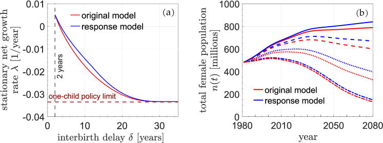
Fig. 8 compares predictions from the standard no-response model (red) to those from a behavioral response model (blue). As expected, behavioral responses blunt the policy-induced decreases in the stationary growth rate (Fig. 8(a)) and the total population (Fig. 8(b)), resulting in higher-than-expected growth and populations. For an imposed $\delta$, a compensatory behavioral response model leads to a higher stationary growth rate. In other words, if the behavioral responses of this example are included, the imposed delay $\delta$ would have to be about 1-2 years longer than in the absence of behavioral response in order to achieve the same overall growth rate (for intermediate delays $\delta\approx 5-15$ years). However, if the refractory period is set very long ($\delta\gtrsim 20$ years), our proposed behavioral responses are futile since females are irreversibly moved past their fertility window.

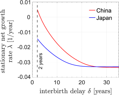
We have examined the effect of applying a refractory period policy in China, which has implemented various birth-control policies over past four decades. To better study this interbirth delay, we apply our model to Japan, which does not have enforced polices on population control. We use Japan’s 2000 population data as a starting point (Statistics Bureau of Japan, 2001). For Japan, we use its 2000 birth rate, which was much lower than that of 1981 China.

Fig. 9 compares the stationary growth rates between China and Japan, imposing different refractory periods $\delta$. Since Japan has a much lower growth rate $\beta_{0}$, with the same $\delta$, the stationary growth rate of Japan is lower than that of China. When $\delta$ is sufficiently large, since each female can have at most one child, the difference between China and Japan diminishes. In fact, the limiting high-$\delta$ stationary growth rate of Japan is slightly higher than that of China. Since the childbearing age is older in Japan, the gap between two successive generations is longer. As observed in Fig. 6(b), under large-$\delta$, sub-replacement conditions, a moderately longer gap between generations can increase the stationary (very long term) growth rate.

References

- Arino [1995] Ovide Arino. A survey of structured cell population dynamics. Acta Biotheoretica, 43(1-2):3–25, jun 1995.
- Bacaër [2011] Nicolas Bacaër. A Short History of Mathematical Population Dynamics. Springer Science & Business Media, 2011.
- Bongaarts and Greenhalgh [1985] John Bongaarts and Susan Greenhalgh. An alternative to the one-child policy in china. Population and Development Review, 11:585–617, 1985.
- Chou and Greenman [2016] Tom Chou and Chris D. Greenman. A hierarchical kinetic theory of birth, death andfission in age-structured interacting populations. Journal of Statistical Physics, 164:49–76, 2016.
- Falkenburg [1973] Donald R. Falkenburg. Optimal control in age dependent populations, pages 112–117. IEEE, New York, NY, 1973.
- Feeney and Yu [1987] Griffith Feeney and Jingyuan Yu. Period parity progression measures of fertility in China. Population Studies, 41(1):77–102, 1987.
- Goodkind [2011] Daniel Goodkind. Child underreporting, fertility, and sex ratio imbalance in China. Demography, 48(1):291–316, 2011.
- Greenhalgh [2004] Susan Greenhalgh. Science, Modernity, and the Making of China’s One-Child Policy. Population and Development Review, 29(2):163–196, jan 2004. ISSN 0098-7921. doi: 10.1111/j.1728-4457.2003.00163.x.
- Greenman [2017] Chris D. Greenman. A path integral approach to age dependent branching processes. Journal of Statistical Mechanics: Theory and Experiment, 2017(3):033101, 2017.
- Greenman and Chou [2016] Chris D. Greenman and Tom Chou. A kinetic theory for age-structured stochastic birth-death processes. Physical Review E, 93(1), jan 2016.
- Gurtin and MacCamy [1974] M. Gurtin and R. C. MacCamy. Non-linear age-dependent population dynamics. Arch. Ration. Mech. Anal., 54:281–300, 1974.
- He et al. [2019] Dan He, Xuying Zhang, Ya’er Zhuang, Zhili Wang, and Yu Jiang. China fertility report, 2006–2016. China Popul. Dev. Stud., 2(4):430–439, 2019.
- Hritonenko and Yatsenko [2010] Natali Hritonenko and Yuri Yatsenko. Age-Structured PDEs in Economics, Ecology, and Demography: Optimal Control and Sustainability. Mathematical Population Studies, 17(4):191–214, 2010.
- Jiang et al. [2017] Da-Quan Jiang, Yue Wang, and Da Zhou. Phenotypic equilibrium as probabilistic convergence in multi-phenotype cell population dynamics. PLoS One, 12(2):e0170916, 2017.
- Kane and Li [2021] Danielle Kane and Ke Li. Fertility cultures and childbearing desire after the two-child policy: evidence from southwest China. Journal of Family Studies, pages 1–19, 2021.
- Kang and Ruan [2021] H. Kang and S. Ruan. Mathematical analysis on an age-structured SIS epidemic model with nonlocal diffusion. J. Math. Biol., 83:5, 2021.
- Kermack and McKendrick [1927] W. O. Kermack and A. G. McKendrick. Contributions to the mathematical theory of epidemics. I. Proceedingsof the Royal Society, 115A:700–721, 1927. ISSN 0092-8240. doi: 10.1016/S0092-8240(05)80040-0.
- Keyfitz and Keyfitz [1997] B. L. Keyfitz and N. Keyfitz. The McKendrick partial differential equation and its uses in epidemiology and population study. Mathl. Comput. Modelling, 26:1–9, 1997.
- Lan and Kuang [2016] Manyu Lan and Yaoqiu Kuang. The impact of women’s education, workforce experience, and the one child policy on fertility in China: a census study in Guangdong, China. Springerplus, 5(1):1–12, 2016.
- Langhaar [1972] H. L. Langhaar. General Population Theory in the Age-Time Continuum. Journal of the Franklin Institute, 293:199–214, 1972.
- Li and Meng [2014] Hongbin Li and Lingsheng Meng. High sex ratio in china: Causes and consequences. In Shenggen Fan, Ravi Kanbur, Shang-Jin Wei, and Xiaobo Zhang, editors, The Oxford Companion to the Economics of China, chapter 81. Oxford Scholarship Online, 2014.
- Li and Wong [2020] Wei Li and Wilson Wong. Advocacy coalitions, policy stability, and policy change in China: The case of birth control policy, 1980–2015. Policy Studies Journal, 48(3):645–671, 2020.
- Man et al. [2021] Wang Man, Shaobin Wang, and Hao Yang. Exploring the spatial-temporal distribution and evolution of population aging and social-economic indicators in China. BMC Public Health, 21(1):1–13, 2021.
- McKendrick [1926] A. G. McKendrick. Applications of mathematics to medical problems. Proc. Edinburgh Math. Soc., 44:98–130, 1926.
- Nie [1999] Jing-Bao Nie. The problem of coerced abortion in China and related ethical issues. Cambridge Quarterly of Healthcare Ethics, 8(4):463–475, 1999.
- Perthame [2007] Benoît Perthame. Transport Equations in Biology. Birkhäuser Basel, Basel, 2007. ISBN 978-3-7643-7841-7.
- Pollard [1973] J.H. Pollard. Mathematical Models for the Growth of Human Population. Cambridge University Press, 1973.
- Population Census Office under the State Council [1985] Population Census Office under the State Council, editor. 1982 Population Census of China (in Chinese). China Statistics Press, 1985.
- Qin and Wang [2017] Yu Qin and Fei Wang. Too early or too late: What have we learned from the 30-year two-child policy experiment in Yicheng, China? Demographic Research, 37:929–956, 2017.
- Song [1980] Jian Song. Bilinear optimal control with constraints in population systems (in Chinese). Zidonghua Xuebao, 6:241–249, 1980.
- Song [1982] Jian Song. Some developments in mathematical demography and their application to the People’s Republic of China. Theoretical Population Biology, 22(3):382–391, 1982. ISSN 0040-5809. doi: 10.1016/0040-5809(82)90051-X.
- Song et al. [1988] Jian Song, Deyong Kong, and Jingyuan Yu. Population System Control. Mathematical and Computational Modelling, 11:11–16, 1988.
- Statistics Bureau of Japan [2001] Statistics Bureau of Japan, editor. 2000 Population Census of Japan (in Japanese). Japan Statistical Society, 2001.
- Tacutu et al. [2018] Robi Tacutu, Daniel Thornton, Emily Johnson, Arie Budovsky, Diogo Barardo, Thomas Craig, Eugene Diana, Gilad Lehmann, Dmitri Toren, Jingwei Wang, Vadim E. Fraifeld, and João P. de Magalhães. Human Ageing Genomic Resources: New and updated databases. Nucleic Acids Research, 46(D1):D1083–D1090, jan 2018. ISSN 1362-4962. doi: 10.1093/nar/gkx1042.
- Tuljapurkar [1983] Shripad Tuljapurkar. Transient dynamics of yeast populations. Mathematical biosciences, 64(2):157–167, 1983.
- von Foerster [1959] H. von Foerster. Some remarks on changing populations in The Kinetics of Cell Proliferation. Springer, 1959.
- Woods and Kilpatrick [2005] C. A. Woods and C. W. Kilpatrick. Infraorder hystricognathi. In D. E. Wilson and D. M. Reeder, editors, Mammal species of the world: A taxonomic and geographic reference, 3rd ed., page 1538. Johns Hopkins University Press, 2005.
- Xia and Chou [2021] Mingtao Xia and Tom Chou. Kinetic theory for structured populations:application to stochastic sizer-timer models of cell proliferation. Journal of Physics A: Mathematical and Theoretical, 54:385601, 2021.
- Xia et al. [2020] Mingtao Xia, Chris D. Greenman, and Tom Chou. PDE models of adder mechanisms in cellular proliferation. SIAM Journal on Applied Mathematics, 80(3):1307–1335, 2020.
- Xu et al. [2009] Fenglian Xu, Liqian Qiu, Colin W Binns, and Xiaoxian Liu. Breastfeeding in China: a review. Int. Breastfeed. J., 4(1):1–15, 2009.
- Zeng et al. [1992] Y. Zeng, P. Tu, B. Gu, Y. Xu, B. Li, and Y. Li. Sex ratio of china’s population deserves attention. China Population Today, 9(6):3–5, 1992.