Modeling the Beam of Gravitational Radiation from a Cosmic String Loop
Abstract
We investigate exact and approximate techniques to calculate the emission of gravitational radiation from cosmic string loops in order to generate beam models covering the entire celestial sphere for a wide range of modes . One approach entails summing over contributions of stationary and nearly-stationary points of individual, factorized, left- and right-moving modes. This “multipoint method” generalizes traditional methods that rely on expansions around exact stationary points of mode products. A second complementary approach extends the method of steepest descent to generate an asymptotic description of the beam as . We present example calculations of the emission of power from cusp-containing loops and compare the results with those obtained by numerically exact techniques as well as by previous approaches. The multipoint method achieves its best results at an intermediate range of modes, improving over previous methods in terms of accuracy. It handles the emission from all regions of the loop not just those near cusps. We demonstrate this capability by making a detailed study of the “pseudocusp” phenomenon.
I Introduction
In certain well-studied cosmological models in string theory [1, 2, 3, 4], a period of inflation may stretch microscopic theory constituents such as F-strings (fundamental strings) or D-branes (branes wrapped on small dimensions) to macroscopic size. Some of these entities span the horizon of the visible universe once inflation ceases, hereafter denoted as “superstrings”111Similar effectively one-dimensional objects arise from symmetry breaking phase transitions in the early universe in Grand Unified Theories (GUTs). The tension of such strings is set by the GUT energy scale. We will denote these strings as “cosmic strings.” Many comments apply equally well to superstrings and cosmic strings. GUT cosmic strings are disfavored by a variety of upper limits on the string tension and by detailed observations of the cosmic microwave background (consistent with adiabatic fluctuations, [84, 83]). Superstrings in braneworld scenarios may possess low tensions that satisfy the known constraints. The stability of different types of superstrings is model dependent.. The horizon-crossing superstrings are the progenitors to a network composed of long strings and smaller closed loops. Minimally coupled strings behave in a relatively simple fashion: a statistical description of the network converges to an attractor solution that is realized when the universe experiences power law expansion as it does during the Big Bang’s conventional radiation and matter eras [6, 7, 8, 9, 10, 11]. The attractor is a scaling solution: long strings collide and form sub-horizon closed loops, the loops oscillate and emit gravitational radiation and decay. All properties measured relative to the horizon are fixed, e.g. the density parameter 222 where is the energy density of the component. for each individual component (long strings, loops and emitted gravitational radiation) remains constant. The statistical properties of the scaling solution are fixed by a few parameters such as the string tension , the number of species or types of different string and the propensity for string intersections to break and rejoin (intercommutation) string elements. The indirect detection of network elements relies on string generated gravitational perturbations that affect Standard model components. One possible scenario is measuring lensing of light-emitting background sources. Direct detection, on the other hand, might involve observing the characteristic gravitational radiation emitted by evaporating strings. The unresolved emission produced by all the network elements in the visible Universe contributes to the stochastic gravitational wave background (SGWB).
Each string loop emits at its fundamental frequency and all higher harmonics. Given a loop’s motion it is straightforward to compute the gravitational radiation emitted mode by mode in different directions on the sky [13]. Low frequency emission from parsec-sized loops might match the bandpass of pulsar detectors whereas high frequency emission from the same loop might fall in the band of frequency sensitivity of a space-based gravitational wave instrument. Low frequency emission is generally directed over a wide angle on the sky, high frequency emission tends to be more narrowly collimated. The goal of this paper is to develop useful approximate tools for determining the gravitational wave emission beamed to the sky by string loops over the entire plausible frequency range of interest. We unite efficient existing methods of calculation at low frequencies with new, more accurate techniques at higher frequencies.
This paper focuses on calculations for loops with cusps and without kinks. It is known that smooth string loops that do not self-intersect generically possess cusps [14], small bits of the string loop that move at ultra-relativistic speeds and beam high frequency gravitational wave emission [15, 16, 17]. If cusps are present on string loops then their emission is expected to dominate the SGWB at high frequencies. The SGWB is an especially important and promising target for space-based gravitational wave detectors like LISA [18]. Nonetheless, the methodology introduced in this paper is potentially applicable to a wider variety of loops such as those that possess kinks [19, 20]. In fact, cosmic string simulations produce mostly kink-filled loops [8, 11] and it will be important to return to apply the new methods to loops with kinks.
The exact calculation of gravitational wave emission must generally be done numerically. However, approximate descriptions [21, 22] are well-developed, especially for the power emitted by high modes. These formalisms consider the emission from a small region on the worldsheet near cusps which is expected to dominate at asymptotically high frequencies. More extensive regions of the worldsheet are important at low frequencies. The methods outlined here build upon and extend existing formalisms to systematically include multiple regions of the loop worldsheet in addition to those near the cusps.
Section II reviews the analytic description of string loop motion, the conditions for cusp formation and the rate at which energy, momentum and angular momentum are carried off by the emission of gravitational radiation. The rates depend upon one-dimensional integrals obtained by factorization of the loop dynamics into the left- and right-moving modes [21, 23, 24]. Finding effective approaches, both analytic and numerical, to evaluate these integrals is the key purpose of this paper. In Section III, we describe two exact methods (real direct, complex direct) and two approximate ones (real multipoint, complex asymptotic) for studying the integrals of interest. In this paper we concentrate on the real multipoint method, providing a detailed analytic exposition. The formalism reproduces existing expressions for emission in the vicinity of a cusp when one is present but applies to a much broader set of physical conditions. We examine necessary criteria for validity. We show that the multipoint method works best in conjunction with other approaches, especially the direct numerical and complex asymptotic methods. In Section IV we examine the application of the multipoint method to a representative set of string loops [25] for a range of emission directions to highlight the loop features that impact accuracy. We show which parts of the mode spectrum and which parts of the celestial sphere are best covered by the various techniques we study. Section V applies the multipoint method to investigate pseudocusp emission by both analytic and numerical means. Section VI compares three approaches (exact numerical integration; cusp-centered calculation – hereafter, “single-point” method; and the new multipoint method) by quantifying accuracy and performance. Section VII gives a general discussion and the applications of the methods and Section VIII summarizes our conclusions.
Conventions used: Throughout the paper, we have assumed . The Greek letters denote spacetime indices of 4-vectors (running from 0 to 3), raised and lowered using the metric with signature (-,+,+,+). In this paper we work to lowest order in the string tension and the required form of the metric is just the Minkowski metric . The 3-vectors are written in bold (eg: is the 3-vector ). The Roman letters denote spatial indices running from 1 to 3 while run from 2 to 3. The letters and are conformal coordinates which parameterize the cosmic string worldsheet.
II Gravitational Wave Emission from a Cosmic String Loop
Cosmic string loops are effectively one-dimensional objects when the curvature scale of the strings is much larger than their thickness. The unperturbed dynamics is described by the Nambu-Goto equation of motion in flat spacetime. The string worldsheet is parameterized by two conformal coordinates and , and represented by . In the conformal gauge, the Nambu-Goto equation of motion is the two-dimensional wave equation,
| (1) |
with constraints set by the Virasoro conditions,
| (2a) | ||||
| (2b) | ||||
For a loop of “invariant” length (defined as , where is the energy of the loop in the center-of-mass frame and is the tension of the loop) the motion is periodic in with a period of and periodic in with a period of . The fundamental domain may be taken to be and .
The general solution to the Nambu-Goto equation of motion is a superposition of left-moving and right-moving modes where
| (3) |
where . Here, are periodic with a period , i.e.
| (4) |
In the center-of-mass frame, we choose the worldsheet coordinate to coincide with the coordinate time i.e. , yields . In this gauge, the Virasoro conditions Eq. (2) become
| (5) |
where the overdot denotes derivative with respect to the corresponding variable. The spacetime vectors obey the relation
| (6) |
Differentiating the above equation leads to the conditions
| (7a) | ||||
| (7b) | ||||
which will be used in Section III.3.
II.1 Cusps
The space of the tangent vectors is the surface of a unit sphere and trace out two separate curves on this unit sphere. If two tangent curves intersect they give rise to a cusp. When that happens a part of the string loop momentarily doubles back on itself in spacetime. Suppose the two tangent curves intersect at
| (8) |
Without loss of generality, define and . It follows from Eq. (3) that
| (9) |
where . The above result implies that the string moves at the speed of light at the cusps in the tangent vector direction. The high Lorentz boost in the regions near the cusp leads to beamed gravitational radiation and quite possibly emission of other particles for non-minimally coupled strings [26, 27, 28, 29].
II.2 Energy, Momentum and Angular Momentum Emitted
A cosmic string loop of length has fundamental frequency where is the oscillation period of the loop. The undamped loop motion is periodic in the center of mass frame and all relevant functions may be expanded in terms of sinusoidal modes with frequencies where . Since we work to lowest non-vanishing order in the string tension the waveform is a linear sum over the sinusoidal modes.
One way to characterize the gravitational wave emission is in terms of the power emitted. The time-averaged power emitted is quadratic in the wave contributions mode-by-mode since all cross terms between different modes average to zero. We write the time-averaged differential power emitted at mode per solid angle as which is a function of , the direction of emission. Figure 1 illustrates the celestial sphere for emission direction overlaying the tangent sphere for tangent curves . Usually we will use spherical polar coordinates and write . The power emitted in a single mode, , is the integral of this differential power over the celestial sphere
| (10) |

The details of the calculation of power emitted have been laid out in [30, 31, 32, 33]. For a cosmic string loop of length , define the one-dimensional integrals,
| (11) |
where and for a given mode number . The vectors and
| (12) | ||||
| (13) |
form a right-handed orthonormal basis with . We will label the 3 elements by below.
The Fourier Transform of the energy-momentum tensor 333For the energy-momentum tensor of the string , the Fourier Transform is obtained as where denotes the spacetime point. of the string loop is
| (14) |
where
| (15) |
The power emitted per unit solid angle in mode along direction is [31]
| (16) |
where each of and take the values 2 and 3 (repeated indices are summed over). In terms of , the differential power is
| (17) |
Generic oscillating string loops radiate not only energy but also momentum and angular momentum. The radiation of net momentum results in a gravitational rocket effect on the string loops which may play an important role in their dynamical motions [35, 36]. The differential rate of radiation of momentum from a cosmic string loop is
| (18) |
Note that the momentum density follows directly from the flux of energy.
The calculation of the rate of radiation of angular momentum from a cosmic string loop is more complicated and has been discussed in detail in [31]. Introducing the integrals
| (19) |
and defining
| (20) |
the Fourier Transform of the first moment of the string energy-momentum tensor is
| (21) |
The radiated angular momentum is orthogonal to . The differential rate of radiated angular momentum per unit solid angle of mode number is
| (22) |
where
| (23) | ||||
| (24) |
Finally, the total radiated energy, momentum and angular momentum are
| (25) | |||||
| (26) | |||||
| (27) |
All three conserved quantities depends upon one dimensional integrals Eq. (11) and Eq. (19). Our focus is on the calculation of these basic quantities. It is important to recognize that the one-dimensional integrals are gauge-dependent but that the combinations giving the physical quantities above are gauge-independent.
II.3 Example Calculations for the Vachaspati-Vilenkin Loop
To sketch the larger context, we examine the power emitted , the rate of emission of momentum and the rate of emission of angular momentum as a function of the mode number for an example cosmic string loop.
For the calculations we select a particular family of loops (which we will refer to as “Vachaspati-Vilenkin loops” to distinguish from other, more symmetric classes of loops introduced in the later sections) with three frequencies and characterized by two parameters and , introduced in [36],
| (28a) | ||||
| (28b) | ||||
For the purposes of demonstration, let us select and . The integrals Eq. (11) and Eq. (19) are performed numerically and combined to calculate and . The differential quantities are integrated over the celestial sphere numerically to give , and according to Eqs. (25), (26) and (27). The left hand panel of Fig. 2 shows the radiated power and the rate of radiated momentum and angular momentum per mode number for this loop up to . The calculated power, rate of radiation of momentum and rate of radiation of angular momentum from the first modes are , and , respectively, in general agreement with [31]. The right hand panel shows the cumulative quantities up to and including mode . Evidently, most of the total radiated power, momentum and angular momentum originates from the lower modes. These will be responsible for the dominant secular change in the loop’s invariant length, center of mass acceleration and spin changes. This particular loop has zero x-components of both and .
We used numerical results to estimate the total power, momentum and angular momentum emitted by the loop from all the modes. We performed quadratures using a regular grid on the celestial sphere for all modes with and using Monte Carlo sampling on the celestial sphere for modes and , , , , , , , and (successive values increase by ). We used linear interpolation of the Monte Carlo results to infer the quadratures for . We extrapolated the results for based on the asymptotic scaling of the integrals for a dominant cusp (large quadratures ). We observed and verified the power law scaling for the numerically calculated quadratures with . Summing these three contributions (explicit, interpolated and extrapolated quadratures) allowed us to estimate the loop’s total power, total rate of radiation of momentum and total rate of radiation of angular momentum: , and , respectively. The quoted range is derived by comparing regular versus Monte Carlo quadrature estimates in the overlap region . Approximately 80% of the total power, momentum magnitude and angular momentum magnitude radiated is sourced by modes with , and , respectively, for this particular loop (the range is as above). Although the upper limits for may appear variable they can be understood in terms of 3 qualitative factors: the intrinsic magnitude of radiated quantities, the possibility of sign cancellations in radiated quantities and the onset of asymptotic variation. Details are quantitatively discussed in Appendix A.
We find at least a factor of 2 variation among different Turok and Vachaspati-Vilenkin loops in terms of the total rates of emission but the qualitative conclusion that lower modes contribute the most remains true.


III Techniques to evaluate
The fundamental step in the calculation of energy, momentum and angular momentum radiated from a cosmic string loop is the estimation of the integrals Eq. (11) and Eq. (19). These are oscillatory integrals with phase . Here we describe two exact and two approximate methods of calculation.
III.1 Direct Evaluation of the Real integral
In general, the integrals cannot be reduced to an explicit closed form (except for a few special cases [36, 31, 30]). At low it is straightforward to use a direct numerical evaluation to derive an “exact” numerical result. The simple trapezoidal rule is exponentially convergent [37] for smooth periodic functions but there are two practical difficulties as grows large. First, the integrand oscillates more and more rapidly and the number of function evaluations needed scales . Second, the cancellation of signed quantities of order unity in the sum accumulates errors that may exceed the exact, small final result. Eventually, higher precision arithmetic must be used in the direct evaluation because the residual answer is so small. Numerical schemes exist that can integrate rapidly oscillating functions [38, 39] but in the next section we will take advantage of the special features of the integrand and develop a customized approach.
Direct numerical schemes related to the Fast Fourier Transform (FFT) were explored in [24, 22]. The methodology may be succinctly summarized as follows: Assume that the integrand, a periodic function in , is represented by discrete samples. A transformation of the original independent variable to a new form absorbs part of the periodic function leaving a pure harmonic (dependent on ) times a weight at the expense of introducing a new grid with uneven spacing. Adopt an interpolation scheme for the weight. Let the new uniform grid have dimension with (values were typical in [24]). Finally, use an FFT of length to perform the quadrature sum. FFT-related methods have the great advantage of computational speed for evaluating a range of mode numbers but suffer from aliasing effects because power at high frequencies is redistributed to low frequencies. As a practical matter, the contamination at low is small because the true power at high frequencies is small compared to the true power at low frequencies, i.e. the induced relative error is small at low frequencies; on the other hand, large results are significantly impacted in terms of relative error. We will see by direct calculation that the accuracy degrades as increases and, in general, the largest mode at which good accuracy can be achieved will satisfy .
III.2 Direct Evaluation by Deformed Complex Contour
Let us focus on the complex analytic properties of the integration of . We simplify the notation and consider one spacetime component and one harmonic of the fundamental frequency. Let , , and . The integral has the form
| (29) |
where and are periodic functions of . For convenience, let so that the exponential above is .
If we were interested in finding an asymptotic approximation to the integral at large we might follow the method of steepest descent [40]. The integrand is a smooth complex function without poles and with various critical points in the complex plane where . The method of steepest descent proceeds by deforming the integration contour to pass through critical point(s) and also requiring that the imaginary part of be constant over the deformed contour. The latter condition suppresses the oscillations of the integrand. Laplace’s method may be used to provide an approximation for the integral along a path for which the integrand is a maximum at the critical point. The technique is commonly used to generate asymptotic approximations (e.g. [40, 41]).
We apply the same ideas here to deform the integration path in the complex plane. A numerical calculation of along the new path will exactly match the direct real calculation along the old path. The new path also provides an asymptotic approximation to by way of the contributions at each of the critical points visited.
Figure 3 illustrates part of the complex plane for an example 444The particulars are not crucial at this point. This example is discussed in greater detail in a following section. It is Case 1 of the mode of a Turok loop with and with direction implied by and .. The original integration path over real is the light gray line that extends from one gray dot at to the other gray dot at . The dashed black, blue and green lines are contours for different fixed . The red dots are critical points with , a subset of all the critical points in the plane for this particular example. The original path is deformed to a connected set of 4 particular segments. The first segment starts at , proceeds to large imaginary (near vertical), then links to colored paths that begin and end at and the last segment returns to the real axis at . The first segment (dashed) has , ascending in the direction with large positive (the integrand is zero). The last segment (also dashed) descends from infinite and large positive to along the contour with . These two segments are identical except for a shift in by . Since and are periodic in the two integrations, one up and one down, exactly cancel each other. The remaining two segments form two looping jumps, from and to with large positive at each end; each segment passes through a critical point at finite with and .

Carrying out an exact evaluation in the complex plane involves three tasks: locating the critical points, finding the complete closed path with piecewise-constant and integrating along the path. The deformed contour need not be found exactly (in the sense that is precisely constant) because any closed contour gives the same integrated result. The advantage of locating a contour with constant is most significant when is large. We have compared numerical results for complex integration along the deformed path to the real integration along the original contour for and achieved agreement at the level of machine precision 555We used the simple trapezoidal rule and also NIntegrate (the generic Mathematica integration recipes) for the real direct method. We used NIntegrate along a numerically determined path for the complex direct integration..
It is worth pointing out a few practical aspects of the numerical integration over the deformed path. The path is independent of so once the path is determined then large batches of can be done efficiently. The integration itself is relatively easy to carry out because, by design, the phase of doesn’t oscillate (the prefactor varies slowly). The maximum of the integrand for each segment occurs near the associated critical point . The concentration of the integrand about the peak is related to – large, positive values imply sharper peaks near the critical point. The peak size sets the scale for additive arithmetic for any integration scheme. If the relative error is (stemming from the truncation error of the integration scheme) then the inferred absolute error . Other than its dependence on the minimum absolute error that can be achieved numerically is constrained by the smallest number that can be represented 666For IEEE-754 double precision normalized floating point we estimate the absolute error .. This is quite different than the residual errors seen in the direct real calculations which involves cancellation of signed quantities of order unity.
III.3 Approximate Real Multipoint Method
The direct numerical schemes for real integration are suitable at small . Here we describe a new method, which turns out to be appropriate for intermediate mode numbers where intermediate means larger than those needing direct methods and smaller than those most accurately evaluated by asymptotic means.
All previous approximations [36, 21, 22] to high mode number integrals exploit the existence of small neighborhoods where the integral builds up because the complex phase doesn’t oscillate too rapidly. These methods are ideal for describing the emission from cusps where the derivatives of both the left and right-moving oscillatory phases vanish. Write the mode conformal coordinates at the cusp as . At the cusp the two tangent vectors are identical. These pick out a special direction which becomes the center of expansion for the approximation. At large the emission is strongest along and falls rapidly away from this special direction on the celestial sphere.
This approach can be modified to yield an improved description in two senses: it will treat emission even when the special direction associated with a cusp does not exist or is irrelevant and it will improve the fidelity of the beam shape. As we will see the improvements also will enable us to extend the description to somewhat lower mode frequencies than previous methods.
For each mode the integral Eq. (11) gets its maximum contribution if aligns with some . But this situation does not hold for either mode for most emission directions. In general, will point away from ,
| (30) |
where corresponds to the deviation for each mode. With our definitions and for unit vectors and so that . For any , there is a corresponding , which is fixed by the choice of , and . Previous authors have generally worked in the limit of small , but we will retain exactly for the moment. The four-vectors and can be Taylor-expanded in a small region around . The largest contribution to the variation of the phase comes from the first three powers of . At the cusp, the leading contribution comes from the cubic term while the linear and quadratic terms are zero. So, for the description of the phase, we shall retain terms up to cubic order in whereas for the prefactor , we will retain the linear term only. With these assumptions, the Taylor expansion of and are
| (31) | ||||
| (32) | ||||
| (33) |
where the terms in the expansion of the phase, Eq. (32), have been rewritten using Eq. (7). We define the coefficients,
| (34) | ||||
| (35) | ||||
| (36) | ||||
| (37) |
and make a change of variables,
| (38) | ||||
| (39) | ||||
| (40) |
Substituting for these quantities in the integral Eq. (11), shifting the origin and extending the integration limits to yields
| (41) |
The integrals
| (42a) | ||||
| (42b) | ||||
can be evaluated analytically. See Appendix B for the explicit expressions.
If aligns exactly with one of the tangent vectors then and the results for that mode simplify as follows:
| (43) | ||||
| (44) | ||||
| (45) | ||||
| (46) | ||||
| (47) | ||||
| (48) | ||||
| (49) | ||||
| (50) | ||||
| (51) | ||||
| (52) |
In this case and .
In the case that the two tangent vectors coincide forming a cusp write . Exact alignment of viewing direction is . Now dropping constants for clarity . From above contain terms and . The stress energy tensor involves symmetrized products like and such expressions involve powers , and . Now [21] showed that all but the last were gauge dependent and could be removed from the stress tensor by a suitable coordinate transformation. In our treatment we do not make any explicit gauge transformations but rely on the fact that we are calculating physical observables even though they are written in terms of gauge dependent quantities. Such observables depend on the appropriate symmetrized combination of the one-dimensional integrals, e.g. the differential power in Eq. (17). Using the Virasoro conditions in Section II we find all the gauge-dependent terms identified by [21] explicitly vanish when we substitute . The final differential cusp power is .
For the cases where aligns with only one of or neither of the tangent vectors the cross terms do not cancel out. Then includes contributions from the lower powers of . The gauge argument in [21] is valid only for the case of a cusp and in the direction of the cusp. It cannot be applied to the more general case. It is important to recognize that the asymptotic behavior as will involve both exponentials and powers of , i.e. one should not conclude that the drop off with is necessarily slower than . We will see, however, that at intermediate the emission in the exact cusp direction need not be dominant.
A similar procedure can be employed to estimate , with the prefactor expanded to linear order and the phase expanded to cubic order.
The cubic expansion Eq. (32) obviously ignores higher order terms. Consider the expansion of the phase up to the 5 order, i.e.,
| (53) |
where are defined in Eq. (34) - Eq. (37) and
| (54) | ||||
| (55) |
Assume that the main contribution for the cubic phase occurs over width . Then the cubic term is dominant if both
| (56) |
The above condition sets an approximate lower bound on given by,
| (57) | ||||
| (58) |
Whenever any of the aforementioned conditions is violated there is no good reason to assume the cubic expansion will provide reliable results. More generally any Taylor series expansion may have a limited radius of convergence so that even if one wanted to extend the method beyond cubic order it might not yield more accurate results.
There are other considerations as well. The Taylor expansion of the prefactor, at linear order must be a good approximation over the contributing width . A necessary condition is
| (59) |
In addition, the width of the peak should be small compared to the size of the fundamental domain () and small compared to the distance to nearby peaks.
Collectively, these inequalities imply the existence of a lower mode for which Eq. (41) is a good approximation. We summarize this by .
We will work exclusively at cubic order for the phase and at linear order for the prefactor and quantify the errors of that approach with respect to exactly known answers.
III.3.1 Finding
For any direction, each value of identifies one center that is responsible for one contribution to the full integral in Eq. (11). In general there can be several distinct centers, i.e. several values of . The principle is to identify all the distinct stationary or nearly-stationary points of the phase responsible for making localized contributions to Eq. (11) and sum these contributions.
The centers of expansion are points where most closely aligns with , i.e. where the derivative of the phase is closest to zero. The quantity of interest has the form
| (60) |
Both and are unit vectors implying . For the case of a cusp, the propagation direction aligns exactly with i.e. . If (no exact alignment) then has to be as close to zero as possible, i.e. should be an isolated point with and a local maximum i.e. . This is what we mean by a near-stationary point. Note that the integral contribution will not be localized at third order if the requirement of a local maximum is dropped. This can be seen heuristically from the third order fit (with ) about a putative center – the cubic fit inevitably gives rise to a distant and distinct stationary point with . All such stationary points are supposed to be found as separate expansion centers. To avoid confusion with the negative signs, we will use as the quantity of interest and so the condition for maxima of translates to condition for minima of . In the following discussions, “minimum (minima)” refers to the minimum (minima) of . In summary, we find all the local minima of for each and sum the individual contributions to approximate the full integral given by Eq. (11). The same recipe may be used to approximate in Eq. (19).
Given a loop and propagation direction the contributions to the functions are calculated according to the following general procedure:
-
•
Select associated with the direction by finding the minima of .
-
•
Expand the phase to cubic order and the prefactor to linear order in about .
- •
-
•
Add up the separate contributions from all the distinct stationary or near-stationary points.
Once the integrals are estimated, they can be combined using Eq. (17) to give for that direction on the celestial sphere.
The key difference between the multipoint method and previous approaches [21, 22] is in the treatment of different points on the string loop. The existing approaches start with the assumption that the cusps dominate the emission at high modes, since they correspond to stationary points in both the phases . To find the emission in regions surrounding the cusp, one expands the phase around the cusp up to a cutoff angle set by the mode number . Beyond this cutoff angle, the emission is exponentially small [21] or calculated using numerical methods [22]. These approaches give accurate results for the emission from a cusp as . In contrast, for each left-moving and right-moving mode the multipoint method finds the expansion point(s) on the loop which contribute the most for a chosen direction on the sphere. These points are not fixed. They need not correspond to a cusp direction and, in addition, a cusp may not even be present. For power calculations the method works separately at the level of the individual one-dimensional integrals and , not the products that define . It handles contributions from both first order (cusps) and second order (non-cusps) stationary points of the phase.
III.4 Asymptotic Complex Integration: Steepest Descent
We make use of the techniques of asymptotic expansion [45] to construct a simple algebraic expression for for the asymptotic limit . Consider the integral in Eq. (29). The first step in the steepest descent method is to determine the critical points on the deformed integration path. At the -th critical point where , and Laplace’s method gives
| (61) |
Here, is the angle that the constant path makes at . It is straightforward to derive higher order approximations as an inverse expansion in powers of :
| (62) | |||||
| (63) |
where , , etc. are functions of , and higher derivatives at the -th critical point. Explicit expressions for , , etc. are given in Appendix C. The numerical evaluation of the asymptotic values is very fast.
III.5 Alignment Limit for the Approximate Methods

Let’s examine the limiting behavior of the real and complex approximations in a particular example in which the beam direction approaches the locus of a tangent vector that traces a great circle on the tangent sphere. Assume the tangent vector lies in the plane . This example is simple enough that we can straightforwardly find the location of the critical points , the integration path and . Let the beam direction be parameterized by spherical polar angles and . Beam directions corresponding to for small imply near alignment.
The critical points of are given by the complex such that and the constant curves that pass through the critical point satisfy for . These are illustrated in Fig. 4.
For slight misalignment there are two distinct critical points, one above and one below the real axis. Note that the solutions are invariant under the change of sign of . The critical points and constant curves above and below the real axis are different solutions, they do not represent positive and negative . As exact alignment of the tangent vector and occurs. Now, the two separate critical points merge on the real axis.
The second derivative of along the path of constant controls whether the critical point is maximum or minimum. implies a peak and implies a bowl. In the figure the critical points with positive imaginary part are peaks, those with negative imaginary parts are bowls. When exact alignment occurs, and the Laplace treatment which relies on the integrand being peaked near the critical point fails. A numerical integration along the constant path will still yield the exact answer but the approximation that the bulk of the integral is contributed near the critical point is incorrect.
Roughly speaking the argument of the exponential that is being integrated has the form and the maximum range of integration is . We would anticipate that must exceed to use the complex asymptotic approach.
Figure 5 depicts the relative errors (with respect to the exact answer) as a function of the mode number for the real multipoint (red) and complex asymptotic (green, brown and pink corresponding to three separate orders , , ) methods. The different panels show different misalignments between the tangent vector and . From top to bottom varies from to in increments of ( in all cases) – exact alignment is . We empirically determine the crossover (hereafter ) such that the real multipoint method yields lower relative errors for and, conversely, that complex asymptotic method yield lower relative errors for .
We can infer from the figure that the size of increases as the angle between the beam direction and the tangent vector decreases and that the crossover point is roughly independent of the order of the complex asymptotic method.
The practical consequences are that for we should adopt a direct or multipoint method while for it will always be advantageous to use the asymptotic methods. In the latter case one would adopt the highest order asymptotic scheme available.
In summary, to calculate the beam shape on the full celestial sphere for we will need two approximate methods, one for near alignment and/or small , the other for misalignment and/or large . This need for multiple methods, somewhat reminiscent of Stokes phenomena, might have been formally anticipated from the qualitatively different mathematical forms that the real multipoint and complex asymptotic methods generate. The real method gives a power law for exact alignment whereas the complex asymptotic method produces a leading, exponential . Consider a sequence of misaligned beams that approach alignment. Evidently one would need many correction terms beyond those of , , etc. multiplying the exponential to reproduce the exact, aligned results.

IV Turok Loop – Multipoint Examples
In this section we will systematically explore the qualitatively different cases that emerge in a practical application of the multipoint calculation. We choose a set of loops introduced by Kibble and Turok in [25]. These loops (which we shall refer to as “Turok loops”) are distinguished from the Vachaspati-Vilenkin loops (Eq. (28)) introduced earlier in their description of . Turok loops involve two frequencies and are characterized by two parameters and ,
| (64a) | ||||
| (64b) | ||||
Both and satisfy the Virasoro condition Eq. (5), and are periodic with a period of . The loop described by Eq. (64) can have two, four or six cusps depending on the values of and as shown in Fig. 6.

IV.1 Calculation of
The integral is calculated in closed form for a given in Appendix E whereas cannot be done in an equivalent manner. We compute numerically exact values of with direct methods and approximate values using the multipoint and asymptotic methods. We focus on the approximate methods here.
IV.1.1 Multipoint Method
Here, we provide a framework for the calculation of using the multipoint method and discuss different scenarios which might arise.
For each direction on the celestial sphere, the first step is determining the value(s) of . Depending on the value of and , the quantity can have either one minimum or three local minima as a function of . For each minimum the value and the mode number determine the local contribution to . In general, we sum over the individual contributions
| (65) |
where denotes the -th minimum. Each individual contribution is based on a cubic fit to the phase derivative in which the integration has been formally extended to . We heuristically refer to the phase derivative as a function of as the “phase curve”. The phase curves are independent of the mode while the integrated quantity which involves the exponential of the phase does depend upon .
We will compare the results of an exact calculation of to the approximate multipoint method for selected values of , and . These choices indirectly control the number of minima, the relative depths and spacings of the minima, the relative size of the cubic and higher order terms near the minima, etc. We present a set of phase curves that covers several qualitatively different situations that arise.
Table IV.1.1 gives a list of six different cases of phase curves which are discussed in more detail below. For this survey we calculate at fixed mode . In all cases the contribution to the (cubic) integral about each peak is narrow in the sense is small compared to the available extent of and the multipoint method is favored over the complex asymptotic method (). We briefly describe the cases:
-
•
Case 1: There is one minimum (see phase curve in Fig. 7), the cubic expansion is good (see the orange dashed line in the plot; set by the 5th order term). Since is close to zero this is a nearly-stationary point. The relative error is %. This case is most similar to situations covered by traditional single point expansion techniques.

Figure 7: Case 1: plot of estimated for at , with a single minimum (). The blue curve is the exact derivative of the phase and the orange dashed curve is the cubic fit to the derivative of the phase about the minimum. -
•
Case 2: Like the previous case there is one minimum (see Fig. 8) with small , however, the phase curve is not well fit by a cubic in the vicinity of the minimum (note that the orange dashed line in the plot misses the shape of the peak; set by 5th order term). The relative error is %, larger than the previous case.

Figure 8: Case 2: plot of estimated for at with a single minimum (). The blue curve is the exact derivative of the phase and the orange dashed curve is the cubic fit about the minimum. The derivative of the phase varies very slowly in the neighborhood of the minimum. -
•
Case 3: Now there are three minima (see Fig. 9). Two have similar magnitudes close to zero and are expected to dominate the sum. They are difficult to distinguish and the cubic fit is not good ( set by the 4th order term near the dominant peaks). The relative error is .

Figure 9: Case 3: plot of estimated for at with three minima (). Two of the minima are similar in magnitude and the derivative of the phase varies very slowly in between them. -
•
Case 4: Like the previous case there are three minima (see Fig. 10) and two have similar magnitudes close to zero. Here, however, the cubic fits to the phase and the linear fit to the prefactor are good (, set by the prefactor), the peaks are better separated and the two dominate the sum. The relative error is %.

Figure 10: Case 4: plot of estimated for at with three minima (). Two minima are similar in magnitude but the derivative of the phase in between them is not flat. -
•
Case 5: Again there are three minima (see Fig. 11) but only one has close to zero, well fit by the cubic and is well separated from the others. The linear fit to the prefactor gives . The relative error is %.

Figure 11: Case 5: plot of estimated for at with three minima (). There is a global minimum which is more prominent than the other two local minima. -
•
Case 6: Figure 12 shows an ideal case for the multipoint method. There are three minima, all with close to zero. The cubic fit is good for each peak. All are well separated. The relative error % and each peak improves the answer. The linear fit to the prefactor is also good ().

Figure 12: Case 6: plot of estimated for at with three minima (). The three minima are of comparable magnitude and all contribute, especially at low .
These cases cover most of the qualitatively different phase curves encountered. The trend of relative errors largely traces the adequacy of the polynomial fits and the independence (degree of separation) of the peaks. The method achieves relative errors when the fit is good and the peaks are not too close to each other.

IV.1.2 Errors as functions of
It is useful to compare the errors of the real multipoint treatment to those of the complex asymptotic treatment. Figure 13 presents results for a selected set of modes for the six cases. Each solution is compared to the exact solution in terms of norm difference divided by norm of exact result. The trends are clear: the relative error for the multipoint method is roughly constant with whereas the relative error of the asymptotic methods decreases with . The multipoint method is superior at small while the asymptotic methods are better at large . The relative error of the highest order asymptotic approximation decreases most rapidly.
In all the illustrated cases the relative error of the multipoint results does not systematically decrease as increases. Nonetheless, the magnitude of the exact, multipoint and asymptotic results all decrease together. In other words, the multipoint answer falls as rapidly as the numerical answer and for many purposes a fixed relative error in an exponentially shrinking quantity is adequate.
IV.1.3 Errors on the celestial sphere
In Section III.5 we showed that for directions on the celestial sphere aligning (or nearly aligning) with tangent curves, the multipoint method must be used. Let’s consider a Turok loop with (same as Case 3) and harmonic and quantify the errors in as a function of position on the celestial sphere. The logarithmic relative errors with respect to an exact numerical answer are shown in a contour representation in Fig. 14. The figure axes are the angles and . Each point represents a direction of . The graph on the left displays contours of the minimum relative error selected from two different approximations: the multipoint and asymptotic () methods. The red dots show where the multipoint treatment is selected, the blue dots are where the asymptotic treatment is. The graph on the right is similar (it contours the logarithmic relative with respect to an exact numerical answer) but takes the multipoint results for and the asymptotic results for . The color coding is identical. Here, we assumed to be the approximate value of where the three asymptotic terms were comparable.
Both plots show that the peak errors lie along the direction of the tangent vector sweep. The asymptotic errors smoothly decrease on both sides away from the peak. The beam is described to roughly 1-10% near the peak (red areas) and with increasing relative (and absolute) accuracy in the asymptotic regime (blue areas).
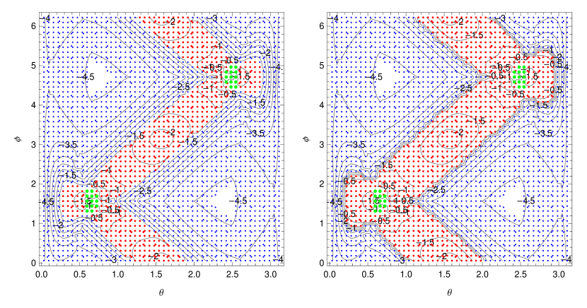
The source of the error near the tangent vector sweep can be traced back to the fit to the phase. Figure 14 shows with green dots the regions of the celestial sphere where the multipoint approximation was used for (i.e. points that violate Eq. 57 because 4th or 5th order terms are important). Note that these points coincide with the largest errors.
IV.1.4 A Schematic Methodological Partition
Finally we want to describe schematically how one might select amongst the different methods mentioned so far. Choice of methodology revolves around considerations of error size and computational timing. Quadrature methods that use increasingly dense point spacing can potentially achieve arbitrarily small errors. Quadratures can be done for individual with adjustable tolerances. In general, point-by-point quadratures are the most flexible in terms of accuracy and also the most time consuming per point. Sets of values can be evaluated en masse by quadrature (e.g. FFT method) for efficiency but then the inaccuracies are linked together and group timings must be considered.
On the other hand, the multipoint and complex asymptotic methodologies provide approximate answers. Mathematically, both are asymptotic expansions. The multipoint method utilizes polynomials to describe the region of the phase function that contributes to the integral; the complex asymptotic analysis approximates the complex phase function by Taylor series expansion of given order. In a practical sense both methods are limited by the finite expansion orders utilized and, in a more fundamental sense, by radius of convergence issues. The methods are not very flexible in terms of accuracy but both are quite fast.
So an elementary consideration is what sort of accuracy is required for a particular application? If very high accuracy is needed then numerical quadrature must be done. Otherwise, multipoint and complex asymptotic may suffice.
A related consideration is whether small absolute errors or small relative errors are needed for the particular application. Note that away from a tangent vector curve the magnitude of the integral answer decreases exponentially as increases. The multipoint method generally achieves constant relative errors as increases whereas the complex asymptotic method gives decreasing relative errors in that limit. One or the other may be sufficient for practical purposes since the magnitude of the answer in that limit is so small.
To illustrate we now pick a point on the celestial sphere for the beam direction and fix the loop parameters. We have selected a direction close to the location of a tangent vector. Figure 15 displays the relative errors of as a function of mode for three methods – the direct evaluation of the real integral using FFT, the multipoint method and the asymptotic method (all with respect to a numerically exact treatment). Two vertical lines and partition the mode space into three ranges. For the case depicted, (due to the accuracy of the linear prefactor) and (inferred by comparing and ). The multipoint method is applicable for and the complex asymptotic method for . The FFT method is not apriori restricted. The mode-by-mode errors are displayed. As increases the lowest errors are provided first by the FFT, then the multipoint and finally the asymptotic method. For the specific numerical choices made the FFT relative errors equal those of the multipoint method at when both are .
We now consider adjustments that might be made. As the figure demonstrates, the accuracy of the FFT method with a transform of fixed length degrades as increases, an aliasing effect related to evaluation of the integrand at unequally spaced points. The FFT may be oversampled by the factor (see Section III.1) whence errors at fixed decrease exponentially as increases. So, by increasing the relative errors for a fixed range of modes may be arbitrarily lowered. If one is satisfied with the typical multipoint error at a given (implicitly in the range ) then the simplest ansatz is to increase until the FFT errors for are less than or equal to that error. Since the FFT relative errors typically increase with while the multipoint errors decrease with the point serves to stitch the two methods together. The FFT method is used for , the multipoint method for and the complex asymptotic method for . (In the figure which is less than . Increasing decreases the error at all and increases.) In patching together the coverage of the three methods we are implicitly assuming that the multipoint method is more efficient per point than the FFT method (see Appendix G for details on timing and other efficiency considerations) and that the complex asymptotic method is as efficient as the multipoint method and also more accurate for . As increases (error level decreases) eventually one transitions directly from the FFT to the asymptotic treatment at .
The case shown in Fig. 15 depicts a well-behaved and consistent decrease in the relative errors for the multipoint and the asymptotic methods as increases. We observe this smooth variation when the beam direction is close to one and only one point on the tangent vector curve. It is not difficult to choose directions that have close encounters with multiple points on the tangent vector curve. This is a common occurrence for directions in the vicinity of self-intersecting points of the tangent vector curve. Interference between multiple individual contributions may induce oscillating relative errors in plots like Fig. 15. Nonetheless, we observe that the envelope of the oscillatory relative errors behaves in a manner similar to those shown. In such cases the partitioning values for should be based on the envelope’s variation.

V A Particular Pseudocusp Example in the Turok loop
Up to now we have concentrated on methods for calculating individual one dimensional integrals like . Now we turn our attention to using the methodology to analyze the pseudocusp phenomena and the energy flux radiated.
V.1 The Phenomena
Consider a Turok loop with parameters . Figure 16 shows the tangent curves for this loop on the unit sphere. There are two cusps with cusp velocities along and ( and for , respectively). In addition to the intersection that creates the cusp itself the tangent curves come close to each other in the plane where the curve has a “nub”.
Figure 17 displays as a function of for calculated by a direct numerical method. The black arrows mark these cusp directions of emission, i.e. such that both . Note that the peaks of the emission don’t align with the cusp directions. The peaks are the “pseudocusps” discussed in [46].


V.2 Qualitative Considerations
Qualitatively, the regions of maximum emission for low mode numbers correspond to points on the unit sphere where the tangent curves come close to each other but do not intersect. The multipoint method approximates and by separately selecting expansion centers from each tangent vector for a given direction . The Euclidean separation between the tangent vectors provides a suggestive means for locating two nearby centers and a strip between them. At true cusps, the tangent vectors intersect and . If is small the two tangent vectors are close to each other and if is a local minimum we may expect, roughly speaking, that the two specific points (one on each tangent vector) might serve as expansion centers for the points along the chord that connects them.
Note, it is merely a matter of convenience whether we specify that expansion center in terms of the values of and for each mode or by means of the vector directions and to the tangent curves or in terms of angular directions on the celestial sphere and . We will use all of these.
In the example, there are two minimal distance solutions: . The corresponding directions are antipodal on the celestial sphere. The first solution has expansion center and for and , respectively; the second solution is and . Now, let us mark the directions and with blue and red arrows respectively for both solutions. The key observation is that the maximum emission occurs in the vicinity of the blue and red arrows.
V.3 Small Angle, Analytic Treatment
We now present a more quantitative approach to this case based on the multipoint method. On the tangent sphere the tangent vectors are symmetric about the surface (the x-plane). In Fig. 16 the “nubs” of the blue curve lies in the x-plane. Construct a small arc in the x-plane that stretches from the to tangent curves (blue to orange along the short segment of a great circle). Consider directions that lie along the arc. Equivalently, in Fig. 17 the arc is a constant slice through the peak. On account of the planar symmetry the centers of the multipoint expansion for and are fixed at for direction along a part of the arc, including the segment that lies between the two tangent curves. This simplifies the application of the multipoint method.
We calculate , and by direct real and multipoint methods. We then provide a simplified analytic and approximate version of the multipoint result to demonstrate the scalings.


Figure 18 shows calculated exactly (solid lines) and by multipoint (dotted) for , and . The abscissa specifies direction along the arc ( is and is ; is the simple interpolated quantity normalized to give a unit vector). The two treatments are in rough agreement bearing in mind that the multipoint is not expected to be applicable at small and its relative accuracy asymptotes to % at large . Note that the peak of shifts from near the tangent lines to a point midway along the arc with increasing .
Since the differential power depends upon products of bilinears in we first examine individual norms like (exact versus multipoint methods) in Fig. 19 and Fig. 20. Both show steep dropoffs away from the expansion directions.
To understand this behavior simplify the analytic multipoint forms by expanding to lowest non-vanishing order all angle-dependent terms in small angle displacements from the tangent directions while leaving the Bessel functions intact. The details are presented in Section H.
The absolute value of the mode functions summarizes a lot of the information of the variation along the arc. We have
| (66) |
for (the angle with respect to the tangent vector which has in this case) and
| (67) |
for (the angle with respect to the tangent vector which has in this case). The analytic and full numerical expressions for the multipoint results are essentially indistinguishable in this example (see plots in Section H).
Terms like scale with the product of the Bessel functions, each having its own centers of expansion. When both terms are exponentially small and the maximum of the product lies between the two tangent lines. Likewise, a local maximum of appears between closely separated tangent lines. This flux must decrease exponentially with . Even if the emission from a pseudocusp exceeds that of a true cusp at given, finite , the emission (between the tangent lines) becomes subdominant as .
V.4 Numerical Investigation
The numerical from the full multipoint are combined using Eq. (17) to give . Figure 21 shows the plot of for the Turok loop with at calculated using the multipoint method. The method qualitatively 777The size of the discrepancy at the peak is consistent with the relative errors seen in the transition from low to intermediate where we would switch from direct to multipoint methods; it reflects the marginal nature of the cubic fit as in Case 3. reproduces the pseudocusps which appear in the profile of calculated by an exact numerical method in Fig. 17.

V.5 Implications
Any method that expands only around a single point like the cusp will be insufficient for this example in which cusp and pseudocusp emit in very different directions. In [22], the authors calculate an analytic expression to approximate for points on the celestial sphere close to the cusps making use of the small-angle approximation. To make comparisons between the various treatments, we extend this single-point method to cover all of the celestial sphere. Discrepancies arising from extending the small-angle approximation to regions away from the cusps are expected but, since the contribution from a cusp falls rapidly as the distance from the cusp increases, these are very small as far as the single-point method is concerned. Figure 22 shows the profile of calculated using the single-point method (extending to angles that cover the whole celestial sphere) for the Turok loop with at . Notice the absence of pseudocusp compared with Fig. 17 and Fig. 21. Local expansion are insufficient to describe distant parts of the string. [22] overcomes the limitation of the single-point method by utilizing it only within a small angle of the cusp and relying on numerical methods outside it. This is feasible when there is an apriori known center. The multipoint method finds expansion points as needed for any direction of emission.
We have shown analytically how pseudocusps vary with and the results are in qualitative agreement with previous works [21, 22, 46]. In Appendix F, we show that the argument for a typical mode varies like . A combination of large , large angle of deviation, and small mode acceleration leads to large Bessel function arguments that give exponentially small results 888We have not given results outside the pair of lines because the expansion points aren’t necessarily fixed and the type of Bessel function can vary when crossing the tangent curve. Nonetheless, we expect similar behavior.. Conversely, when is small, when the two tangent curves come close to each other, move slowly and have large acceleration then the results need not be small. This is qualitatively in accordance with [46].

VI A Survey of Using Numerical, Multipoint and Single-Point Methods
We now seek to quantify the accuracy of the multipoint method in a systematic, albeit empirical manner. This is necessary because of the difficulty setting forth apriori requirements for accuracy (e.g. discussion of linear and cubic expansions in Section III.3). We will compute over the entire celestial sphere for a few example sets of parameters for the Turok loop described by Eq. (64), using an numerically exact method, the multipoint method and the single-point method. The following procedure defines the evaluation metric:
-
•
For each set of parameters and each mode number , the maximum value of power emitted per solid angle, , over the entire celestial sphere is calculated by a numerically exact procedure.
-
•
For the same loop and mode number, we find the maximum difference over the entire celestial sphere between the values of computed by numerically exact and by the approximate methods: where stands for the multipoint method or the single-point method and exact is the numerical evaluation.
-
•
We summarize method fidelity in terms of the maximum absolute difference (MAD) (expressed in terms of per steradian) and the maximum relative difference (MRD) where is the method.
We plot MAD and MRD vs. in log-log scale for the two methods and compare the trends for four different illustrative cases involving two or six cusps. Cases with two and six cusps occupy finite areas in Fig. 6 while those with four cusps only occur on boundaries 999To be precise, for most and the two tangent curves intersect at two or six points. Consider the separation along the plane. For each value of , there is a specific value of for which the curves intersect in the plane and form a cusp. These solutions yield loops with four cusps.. We shall not discuss these boundary cases separately – the conclusions drawn from them are similar.
VI.1 Two Cusps, Well-Separated Tangent Curves
Consider the Turok loop with . For this loop, the tangent curves and intersect at two points on the unit sphere, forming two cusps, as shown in Fig. 23. The velocities point along the and axes respectively i.e. along . The tangent curves are elsewhere well-separated. We don’t expect pseudocusps so the single-point and multipoint method should be equally effective.


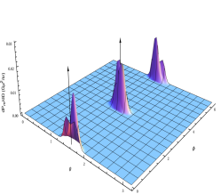

Figure 24 shows plots of calculated numerically for three different mode numbers . Most emission comes from a small region near the direction . The beam shape is more complicated than a filled cone with solid opening angle [21]. In fact, there are two prominent subpeaks. These scale down as mode number increases in the sense that the separation of the subpeaks and the width of the subpeaks all shrink together. The beam is asymptotically self-similar. All qualitative features of the plots seen in the numerical calculation are reproduced by both the multipoint method and the single-point method but there are quantitative differences. Figure 25 shows MAD and MRD vs. mode number. While both the multipoint method and the single-point method are in good agreement with each other and with the numerical calculation, the former performs marginally better than the latter. The multipoint method reaches a MRD of 0.5% by mode number while the single-point method reaches the same by mode number . Both methods yield more accurate results for higher modes.

VI.2 Two Cusps with Pseudocusp Effect
As parameters vary many different “close encounters” between the two tangent curves may occur. In some cases the tangent curves approach at a few specific points (like the “nub” in our previous example that corresponds to a local minimum in the distance of separation and gives rise to a localized pseudocusp) while in others the curves may be roughly parallel over some range of . If the angle between the two curves that cross to give a true cusp is small then the possibility arises for an extended emission region in the vicinity of the cusp itself.
As an example consider the Turok loop with , shown in Fig. 26. This loop has two cusps with velocities pointing along . For asymptotically large , the maximum emission is expected to be along these directions on the celestial sphere. Unlike the previous example, in the plane the two tangent vectors are at maximum distance from each other (the “nub” on is far from ) and they approach closely for an extended range near the cusp only because they form an acute angle at the point of intersection.


Figures 27, 28 and 29 show the plots of computed using the numerical, the multipoint and the single-point method for this loop at modes . The emission is maximum at , appearing at near the nub. That region migrates towards the cusps on either side as increases. Higher requires smaller angles of separation between the tangent curves.
The multipoint method, depicted in Fig. 28, reproduces the trends. For the maximum value of near the nub computed using this method is off from the value computed numerically by (the size of the discrepancy is consistent with the relative errors seen in the transition from low to intermediate where we would switch from direct to multipoint methods). As increases the differences shrink. The single-point method, with center of expansion at the cusp itself, misses the most prominent and distant pseudocusp near the nub but the size of the error decreases as increases once the cusp becomes prominent.

Figure 30 shows the MAD and MRD for both methods as a function of the mode number. The multipoint method reaches a MRD of 6% by mode number while the single-point method reaches the same by mode number, . The dip in the MAD and MRD for both methods at has a simple explanation. For , the maximum differences between each of the approximate methods and the numerical method occur near the nub. Because the multipoint method better reproduces the pseudocusp there, the errors are smaller compared with those of the single-point method. For the maximum differences occur closer to the cusps which are picked up by both the methods. Both methods get more accurate near the cusps and the differences decrease. But the multipoint method still fares better overall for this case.
VI.3 Six Cusps with Pseudocusp Effect
For the Turok loops with six cusps, there exists a range of parameters where the two tangent vectors are close to each other (see Fig. 6). Consider the Turok loop described by . The tangent curves intersect each other at six points on the unit sphere giving rise to six cusps, as shown in Fig. 31. In addition to the cusps, the two tangent curves also approach each other along the plane (). These generate extended emission. We omit detailed renditions of the emission and simply use MAD and MRD to quantify the accuracy.

Figure 32 shows the MAD and MRD for the two analytic methods. The MAD decreases more or less consistently with . The MRD also decreases over a large range of , but since it involves scaling the MAD by the maximum value of , there are minor variations when the decrease in MAD is not proportional to the decrease in . The MRD reaches % by for the multipoint method but it is an order of magnitude bigger for the single-point method. The maximum differences in both cases are found near the pseudocusps for . In summary, the multipoint method yields more accurate results as it takes into account the pseudocusps which the single-point method does not describe.

VI.4 Six Well-Separated Cusps
For larger values of , the tangent curve becomes more wiggly and the separation between the cusps increases. Compared to the previous case, larger create larger separation between the tangent curves in between the cusps. As an example, consider the Turok loop described by . Figure 33 shows the two tangent curves for this loop. The six cusps are well-separated on the unit sphere and the distance between the two curves at is also larger than in the previous case.


We expect that pseudocusps will not play as big a role as in the previous cases (Section VI.2 and Section VI.3). The MRDs are still smaller for the multipoint method, as shown in Fig. 34. The MRD for the multipoint method reaches % by whereas for the single-point method, it reaches the same range only by .
VI.5 Implications
For all four cases described, the multipoint method fares better than the single-point methods in the calculation of . These four cases cover the main situations observed for Turok loops. The multipoint method yields lower MRDs than the single-point method overall, but the difference is marked for cases involving pseudocusps. The advantage of the multipoint method is that it takes into account regions of the loop away from the cusps, which play an important role in the low to intermediate mode number range. In addition, it improves the accuracy of the beam shape even when only cusps are present.
VII Discussion
We have considered the gravitational wave emission from a cosmic string loop. All calculations reduce to evaluating one-dimensional integrals over the left- and right-moving modes of the string. Our goal was to develop a network of techniques to handle the emission over the entire range of harmonics and over the whole celestial sphere. The techniques are directly relevant to the calculation of waveforms of the outgoing gravitational waves and the evaluation of fluxes of radiated conserved quantities.
Here, we have concentrated on applying the techniques to calculating the frequency-dependent emission of energy, momentum and angular momentum. The SGWB generated by cosmic strings at a range of redshifts is one of the principal applications. If that signal is experimentally detected it will probe various cosmological features such as the radiation-to-matter transition, the number of relativistic degrees of freedom at different redshifts and other interesting questions related to the properties of the strings themselves [18]. There are a wide range of experiments that can potentially probe the SGWB for frequencies between and Hz. These include pulsar timing arrays (NANOGRAV [50], EPTA [51], IPTA [52], InPTA [53], PPTA [54], CPTA [55] and MeerKAT PTA [56]) and interferometric ground-based detector networks [57] including various individual interferometers (LIGO and Advanced LIGO [58, 59], VIRGO [60], KAGRA [61], IndIGO [62]) and co-located interferometers (Holometer [63]). Proposed space-based experiments (LISA [64], ASTROD-GW [65], BBO [66], DECIGO [67], TianGO [68] and TianQind [69]) and proposed ground-based detectors (ET [70, 71, 72], Cosmic Explorer [73, 74]) should extend the sensitivity and frequency coverage.
To give an example when the beam modeling of a source becomes directly relevant to observations we will consider the possibility that a relatively nearby string loop radiates and is detected in the face of the confusion of a cosmologically produced SGWB [75, 76, 77]. This will illustrate how each of the separate analytic regimes describing the beam may play a role in a full analysis of the loop’s putative signal.
Today, local string loops have a characteristic size pc for tension . (This size corresponds to a loop that radiates its entire mass by emission of gravitational radiation in a period of time equal to the age of the Universe). In the network scaling solution a fixed number of loops with size equal to a fraction of the horizon form at each epoch. The oldest, surviving loops in the Universe have the highest number density today. For loop size the most numerous and typical loops have of order 1. Given an instrument sensitive to frequency we infer the harmonic of interest . The characteristic harmonic of the emission of a nearby (not cosmologically distant) loop is where is the age of the Universe and , a dimensionless constant characterizing the efficacy of the loop’s emission of gravitational waves. Quantitatively, . We have calculated the expected number of observable, nearby loops in a homogeneous Universe as a function of , and according to two different detection criteria: (1) the energy flux in the loop exceeds that of the SGWB flux and (2) an experiment of fixed total duration yields a high S/N result in a template search for a harmonic source (a particular mode of the string emission) where the background noise is the SGWB. In these idealized analyses neither instrumental effects nor other astrophysical sources impede the detection of the nearby loop and the results are “best case” scenarios. The inhomogeneity of the distribution of loop sources in the Universe is ignored. We will present details elsewhere but simply summarize that the characteristic range of harmonics of the detections agree with the estimate above. An experiment like LISA with Hz is potentially sensitive to harmonics emitted by a single loop up to . It is important to emphasize that the numbers of detections forecast differ markedly for the two criteria and are strong functions of the observing frequency. In addition, all numbers are sensitive to other factors including local clustering of string loops (see differing estimates in [78, 79]) and the degree of enhancement of superstring numbers over that of normal strings [80, 81]. The important point is simply that one expects loops to emit in a large range of .
To handle the integrals over a range of we have discussed three types of techniques: direct calculation (simple numerical quadrature, FFT-mediated quadratures and deformed complex contour methods), stationary point and near-stationary point approximations (multipoint method) and asymptotic approximations (Laplace’s method).
These methods are naturally suitable for covering complementary ranges of mode numbers as depicted in Fig. 15. Direct numerical quadrature is appropriate at low modes where the relevant integrals are mildly oscillatory. The FFT-mediated approach has the efficiency of handling multiple modes together but the accuracy is limited by aliasing effects as increases.101010We have also validated the capability of the method of steepest descent to produce exact calculations, equivalent to direct numerical integration, but not included it in the set of comparisons and will report the details elsewhere.
All direct techniques suffer from increasing calculational complexity as increases. We have introduced two approximate methods well suited to larger : the multipoint method and the asymptotic method. The multipoint method builds upon the existing techniques [21, 22] but is not restricted to cusps and, in particular, is ideal for analyzing the emission away from cusps such as that associated with pseudocusps.
Our multipoint exploration of the pseudocusp phenomena demonstrates that pseudocusps can dominate cusps at intermediate but are subdominant at large . This is in agreement with the previous works [21, 22, 46]. The strength of the pseudocusp emission is influenced by multiple factors – the angle of separation between the tangent curves on the celestial sphere and the velocity and acceleration of the tangent vectors. These set the magnitude and the variation of (refer to Appendix H for details) which is the key element of the multipoint approximation.
We have investigated the behavior of the multipoint method over a wide range of and assessed its accuracy. The absolute scale of the beam emission decreases as increases but the relative errors plateau at values of for large . Depending upon the application, it may be sufficient to utilize the results without further worry – they have small absolute errors but large relative errors. In any case, the multipoint method compares favorably with all other existing techniques not only away from cusps but also in the direction of cusps. For example, it provides more accurate cusp beam shapes than existing methods.
We also introduced an asymptotic analysis based on locating the steepest descent contours in the complex plane and treating the one-dimensional integral by means of Laplace’s method. This was particularly effective at large and yielded decreasing relative errors. The most accurate treatment of the beam should switch from the multipoint (or direct) methods to the asymptotic method at large . The transition is not simple. It depends not only upon but also upon the alignment of the viewing angle and the tangent directions. The closer the direction is to exact alignment the larger the mode number must be for the asymptotic analysis to become accurate. We have provided an empirical method to determine the transition by examining the results that are generated by successive orders of the asymptotic method.
Elsewhere we will return to the problem of constructing time-dependent waveforms.
VIII Conclusion
We have introduced two new methods to approximate the emission of gravitational radiation from a cosmic string loop. The asymptotic method makes use of the method of steepest descent to approximate the values of the integrals and matches the exact answer as . The multipoint method performs best for an intermediate range of modes . It generally gives better results than other approximate methods. It improves upon single-point methods (which focus mainly on the cusps formed on the loop) by including new regions of the loop which contribute to the emission at lower modes. It extends the range of mode numbers for which the emission can be reliably calculated.
A combination of direct numerical methods at low modes, the multipoint method at intermediate modes and the asymptotic method at high modes has the potential to provide a complete, calculable model for gravitational wave emission from a single cosmic string loop.
IX Acknowledgements
DC thanks Soumyajit Bose, Liam McAllister and Barry Wardell for useful conversations. NS thanks the Cornell Department of Astronomy for summer graduate fellowship over June 2023.
References
- Jones et al. [2002] N. Jones, H. Stoica, and S.-H. Tye, Brane interaction as the origin of inflation, Journal of High Energy Physics 2002, 051 (2002).
- Sarangi and Tye [2002] S. Sarangi and S.-H. Tye, Cosmic string production towards the end of brane inflation, Physics Letters B 536, 185 (2002).
- Kachru et al. [2003] S. Kachru, R. Kallosh, A. Linde, J. Maldacena, L. McAllister, and S. P. Trivedi, Towards inflation in string theory, Journal of Cosmology and Astroparticle Physics 2003 (10), 013.
- Copeland et al. [2004] E. J. Copeland, R. C. Myers, and J. Polchinski, Cosmic f- and d-strings, Journal of High Energy Physics 2004, 013 (2004).
- Note [1] Similar effectively one-dimensional objects arise from symmetry breaking phase transitions in the early universe in Grand Unified Theories (GUTs). The tension of such strings is set by the GUT energy scale. We will denote these strings as “cosmic strings.” Many comments apply equally well to superstrings and cosmic strings. GUT cosmic strings are disfavored by a variety of upper limits on the string tension and by detailed observations of the cosmic microwave background (consistent with adiabatic fluctuations, [84, 83]). Superstrings in braneworld scenarios may possess low tensions that satisfy the known constraints. The stability of different types of superstrings is model dependent.
- Vachaspati and Vilenkin [1984] T. Vachaspati and A. Vilenkin, Formation and evolution of cosmic strings, Phys. Rev. D 30, 2036 (1984).
- Albrecht and Turok [1985] A. Albrecht and N. Turok, Evolution of cosmic strings, Phys. Rev. Lett. 54, 1868 (1985).
- Bennett and Bouchet [1988] D. P. Bennett and F. m. c. R. Bouchet, Evidence for a scaling solution in cosmic-string evolution, Phys. Rev. Lett. 60, 257 (1988).
- Sakellariadou [2005] M. Sakellariadou, A note on the evolution of cosmic string/superstring networks, Journal of Cosmology and Astroparticle Physics 2005 (04), 003.
- Urrestilla and Vilenkin [2008] J. Urrestilla and A. Vilenkin, Evolution of cosmic superstring networks: a numerical simulation, Journal of High Energy Physics 2008, 037 (2008).
- Blanco-Pillado et al. [2011] J. J. Blanco-Pillado, K. D. Olum, and B. Shlaer, Large parallel cosmic string simulations: New results on loop production, Physical Review D 83, 10.1103/physrevd.83.083514 (2011).
- Note [2] where is the energy density of the component.
- Weinberg [1972] S. Weinberg, Gravitation and Cosmology: Principles and Applications of the General Theory of Relativity (John Wiley and Sons, New York, 1972).
- Thompson [1988] C. Thompson, Dynamics of cosmic string, Phys. Rev. D 37, 283 (1988).
- Turok [1984] N. Turok, Grand unified strings and galaxy formation, Nuclear Physics B 242, 520 (1984).
- Vachaspati [1987] T. Vachaspati, Gravity of Cosmic Loops, Phys. Rev. D 35, 1767 (1987).
- Damour and Vilenkin [2000] T. Damour and A. Vilenkin, Gravitational wave bursts from cosmic strings, Phys. Rev. Lett. 85, 3761 (2000).
- Auclair et al. [2020] P. Auclair, J. J. Blanco-Pillado, D. G. Figueroa, A. C. Jenkins, M. Lewicki, M. Sakellariadou, S. Sanidas, L. Sousa, D. A. Steer, J. M. Wachter, and S. Kuroyanagi, Probing the gravitational wave background from cosmic strings with LISA, Journal of Cosmology and Astroparticle Physics 2020 (04), 034.
- Garfinkle and Vachaspati [1988] D. Garfinkle and T. Vachaspati, Fields due to kinky, cuspless, cosmic loops, Phys. Rev. D 37, 257 (1988).
- Allen and Ottewill [2001a] B. Allen and A. C. Ottewill, Waveforms for gravitational radiation from cosmic string loops, Phys. Rev. D 63, 063507 (2001a).
- Damour and Vilenkin [2001] T. Damour and A. Vilenkin, Gravitational wave bursts from cusps and kinks on cosmic strings, Physical Review D 64, 10.1103/physrevd.64.064008 (2001).
- Blanco-Pillado and Olum [2017] J. J. Blanco-Pillado and K. D. Olum, Stochastic gravitational wave background from smoothed cosmic string loops, Physical Review D 96, 10.1103/physrevd.96.104046 (2017).
- Garfinkle and Vachaspati [1987] D. Garfinkle and T. Vachaspati, Radiation from kinky, cuspless cosmic loops, Phys. Rev. D 36, 2229 (1987).
- Allen and Shellard [1992] B. Allen and E. P. S. Shellard, Gravitational radiation from cosmic strings, Phys. Rev. D 45, 1898 (1992).
- Kibble and Turok [1982] T. Kibble and N. Turok, Self-intersection of cosmic strings, Physics Letters B 116, 141 (1982).
- Vilenkin and Vachaspati [1987] A. Vilenkin and T. Vachaspati, Electromagnetic radiation from superconducting cosmic strings, Phys. Rev. Lett. 58, 1041 (1987).
- Blanco-Pillado and Olum [2001] J. Blanco-Pillado and K. D. Olum, Electromagnetic radiation from superconducting string cusps, Nuclear Physics B 599, 435 (2001).
- Peloso and Sorbo [2003] M. Peloso and L. Sorbo, Moduli from cosmic strings, Nuclear Physics B 649, 88 (2003).
- Long et al. [2014] A. J. Long, J. M. Hyde, and T. Vachaspati, Cosmic strings in hidden sectors: 1. radiation of standard model particles, Journal of Cosmology and Astroparticle Physics 2014 (09), 030.
- Burden [1985] C. Burden, Gravitational radiation from a particular class of cosmic strings, Physics Letters B 164, 277 (1985).
- Durrer [1989] R. Durrer, Gravitational angular momentum radiation of cosmic strings, Nuclear Physics B 328, 238 (1989).
- Vilenkin and Shellard [2000] A. Vilenkin and E. P. S. Shellard, Cosmic Strings and Other Topological Defects (Cambridge University Press, 2000).
- Allen and Ottewill [2001b] B. Allen and A. C. Ottewill, Waveforms for gravitational radiation from cosmic string loops, Physical Review D 63, 10.1103/physrevd.63.063507 (2001b).
- Note [3] For the energy-momentum tensor of the string , the Fourier Transform is obtained as where denotes the spacetime point.
- Hogan and Rees [1984] C. J. Hogan and M. J. Rees, Gravitational interactions of cosmic strings, Nature 311, 109 (1984).
- Vachaspati and Vilenkin [1985] T. Vachaspati and A. Vilenkin, Gravitational radiation from cosmic strings, Phys. Rev. D 31, 3052 (1985).
- Trefethen and Weideman [2014] L. N. Trefethen and J. A. Weideman, The exponentially convergent trapezoidal rule, SIAM Rev. 56, 385 (2014).
- Levin [1996] D. Levin, Fast integration of rapidly oscillatory functions, Journal of Computational and Applied Mathematics 67, 95 (1996).
- Levin [1997] D. Levin, Analysis of a collocation method for integrating rapidly oscillatory functions, Journal of Computational and Applied Mathematics 78, 131 (1997).
- Stein and Shakarchi [2010] E. Stein and R. Shakarchi, Complex Analysis, Princeton lectures in analysis (Princeton University Press, 2010).
- de Bruijn [1981] N. de Bruijn, Asymptotic Methods in Analysis, Bibliotheca mathematica (Dover Publications, 1981).
- Note [4] The particulars are not crucial at this point. This example is discussed in greater detail in a following section. It is Case 1 of the mode of a Turok loop with and with direction implied by and .
- Note [5] We used the simple trapezoidal rule and also NIntegrate (the generic Mathematica integration recipes) for the real direct method. We used NIntegrate along a numerically determined path for the complex direct integration.
- Note [6] For IEEE-754 double precision normalized floating point we estimate the absolute error .
- Erdélyi [1956] A. Erdélyi, Asymptotic Expansions, Dover Books on Mathematics (Dover Publications, 1956).
- Stott et al. [2017] M. J. Stott, T. Elghozi, and M. Sakellariadou, Gravitational wave bursts from cosmic string cusps and pseudocusps, Physical Review D 96, 10.1103/physrevd.96.023533 (2017).
- Note [7] The size of the discrepancy at the peak is consistent with the relative errors seen in the transition from low to intermediate where we would switch from direct to multipoint methods; it reflects the marginal nature of the cubic fit as in Case 3.
- Note [8] We have not given results outside the pair of lines because the expansion points aren’t necessarily fixed and the type of Bessel function can vary when crossing the tangent curve. Nonetheless, we expect similar behavior.
- Note [9] To be precise, for most and the two tangent curves intersect at two or six points. Consider the separation along the plane. For each value of , there is a specific value of for which the curves intersect in the plane and form a cusp. These solutions yield loops with four cusps.
- Brazier et al. [2019] A. Brazier et al., The NANOGrav Program for Gravitational Waves and Fundamental Physics, (2019), arXiv:1908.05356 [astro-ph.IM] .
- Desvignes et al. [2016] G. Desvignes et al. (EPTA), High-precision timing of 42 millisecond pulsars with the European Pulsar Timing Array, Mon. Not. Roy. Astron. Soc. 458, 3341 (2016), arXiv:1602.08511 [astro-ph.HE] .
- Verbiest et al. [2016] J. P. W. Verbiest et al., The International Pulsar Timing Array: First Data Release, Mon. Not. Roy. Astron. Soc. 458, 1267 (2016), arXiv:1602.03640 [astro-ph.IM] .
- Joshi et al. [2018] B. C. Joshi et al., Precision pulsar timing with the ORT and the GMRT and its applications in pulsar astrophysics 10.1007/s12036-018-9549-y (2018).
- Manchester et al. [2013] R. N. Manchester et al., The Parkes Pulsar Timing Array Project, Publ. Astron. Soc. Austral. 30, 17 (2013), arXiv:1210.6130 [astro-ph.IM] .
- Xu et al. [2023] H. Xu et al., Searching for the Nano-Hertz Stochastic Gravitational Wave Background with the Chinese Pulsar Timing Array Data Release I, Res. Astron. Astrophys. 23, 075024 (2023), arXiv:2306.16216 [astro-ph.HE] .
- Miles et al. [2023] M. T. Miles et al., The MeerKAT Pulsar Timing Array: first data release, Mon. Not. Roy. Astron. Soc. 519, 3976 (2023), arXiv:2212.04648 [astro-ph.HE] .
- Abbott et al. [2018] B. P. Abbott et al. (KAGRA, LIGO Scientific, Virgo, VIRGO), Prospects for observing and localizing gravitational-wave transients with Advanced LIGO, Advanced Virgo and KAGRA, Living Rev. Rel. 21, 3 (2018), arXiv:1304.0670 [gr-qc] .
- Aasi et al. [2015] J. Aasi et al. (LIGO Scientific), Advanced LIGO, Class. Quant. Grav. 32, 074001 (2015), arXiv:1411.4547 [gr-qc] .
- Abbott et al. [2017] B. P. Abbott et al. (LIGO Scientific), Exploring the Sensitivity of Next Generation Gravitational Wave Detectors, Class. Quant. Grav. 34, 044001 (2017), arXiv:1607.08697 [astro-ph.IM] .
- Acernese et al. [2015] F. Acernese et al. (VIRGO), Advanced Virgo: a second-generation interferometric gravitational wave detector, Class. Quant. Grav. 32, 024001 (2015), arXiv:1408.3978 [gr-qc] .
- Akutsu et al. [2021] T. Akutsu et al. (KAGRA), Overview of KAGRA: Detector design and construction history, PTEP 2021, 05A101 (2021), arXiv:2005.05574 [physics.ins-det] .
- Unnikrishnan [2023] C. S. Unnikrishnan, LIGO-India: A Decadal Assessment on Its Scope, Relevance, Progress, and Future, (2023), arXiv:2301.07522 [astro-ph.IM] .
- Chou et al. [2017] A. Chou et al. (Holometer), The Holometer: An Instrument to Probe Planckian Quantum Geometry, Class. Quant. Grav. 34, 065005 (2017), arXiv:1611.08265 [physics.ins-det] .
- Babak et al. [2021] S. Babak, A. Petiteau, and M. Hewitson, LISA Sensitivity and SNR Calculations, (2021), arXiv:2108.01167 [astro-ph.IM] .
- Ni [2013] W.-T. Ni, ASTROD-GW: Overview and Progress, Int. J. Mod. Phys. D 22, 1341004 (2013), arXiv:1212.2816 [astro-ph.IM] .
- Crowder and Cornish [2005] J. Crowder and N. J. Cornish, Beyond LISA: Exploring future gravitational wave missions, Phys. Rev. D 72, 083005 (2005), arXiv:gr-qc/0506015 .
- Kawamura et al. [2021] S. Kawamura et al., Current status of space gravitational wave antenna DECIGO and B-DECIGO, PTEP 2021, 05A105 (2021), arXiv:2006.13545 [gr-qc] .
- Kuns et al. [2020] K. A. Kuns, H. Yu, Y. Chen, and R. X. Adhikari, Astrophysics and cosmology with a decihertz gravitational-wave detector: TianGO, Phys. Rev. D 102, 043001 (2020), arXiv:1908.06004 [gr-qc] .
- Torres-Orjuela et al. [2023] A. Torres-Orjuela, S.-J. Huang, Z.-C. Liang, S. Liu, H.-T. Wang, C.-Q. Ye, Y.-M. Hu, and J. Mei, Detection of astrophysical gravitational wave sources by TianQin and LISA, (2023), arXiv:2307.16628 [gr-qc] .
- Punturo et al. [2010a] M. Punturo et al., The third generation of gravitational wave observatories and their science reach, Class. Quant. Grav. 27, 084007 (2010a).
- Punturo et al. [2010b] M. Punturo et al., The Einstein Telescope: A third-generation gravitational wave observatory, Class. Quant. Grav. 27, 194002 (2010b).
- Hild et al. [2011] S. Hild et al., Sensitivity Studies for Third-Generation Gravitational Wave Observatories, Class. Quant. Grav. 28, 094013 (2011), arXiv:1012.0908 [gr-qc] .
- Evans et al. [2021] M. Evans et al., A Horizon Study for Cosmic Explorer: Science, Observatories, and Community, (2021), arXiv:2109.09882 [astro-ph.IM] .
- Reitze et al. [2019] D. Reitze, R. X. Adhikari, S. Ballmer, B. Barish, L. Barsotti, G. Billingsley, D. A. Brown, Y. Chen, D. Coyne, R. Eisenstein, M. Evans, P. Fritschel, E. D. Hall, A. Lazzarini, G. Lovelace, J. Read, B. S. Sathyaprakash, D. Shoemaker, J. Smith, C. Torrie, S. Vitale, R. Weiss, C. Wipf, and M. Zucker, Cosmic explorer: The u.s. contribution to gravitational-wave astronomy beyond ligo (2019), arXiv:1907.04833 [astro-ph.IM] .
- DePies and Hogan [2009] M. R. DePies and C. J. Hogan, Harmonic gravitational wave spectra of cosmic string loops in the galaxy (2009), arXiv:0904.1052 [astro-ph.CO] .
- Khakhaleva-Li and Hogan [2020] Z. Khakhaleva-Li and C. J. Hogan, Will lisa detect harmonic gravitational waves from galactic cosmic string loops? (2020), arXiv:2006.00438 [astro-ph.CO] .
- Martinez and Kamai [2020] J. G. C. Martinez and B. Kamai, Searching for MHz gravitational waves from harmonic sources, Class. Quant. Grav. 37, 205006 (2020), arXiv:2010.06118 [astro-ph.IM] .
- Chernoff [2009] D. F. Chernoff, Clustering of Superstring Loops, (2009), arXiv:0908.4077 [astro-ph.CO] .
- Jain and Vilenkin [2020] M. Jain and A. Vilenkin, Clustering of cosmic string loops, JCAP 09, 043, arXiv:2006.15358 [astro-ph.CO] .
- Chernoff and Tye [2015] D. F. Chernoff and S. H. H. Tye, Inflation, string theory and cosmic strings, Int. J. Mod. Phys. D 24, 1530010 (2015), arXiv:1412.0579 [astro-ph.CO] .
- Chernoff and Tye [2018] D. F. Chernoff and S. H. H. Tye, Detection of Low Tension Cosmic Superstrings, JCAP 05, 002, arXiv:1712.05060 [astro-ph.CO] .
- Note [10] We have also validated the capability of the method of steepest descent to produce exact calculations, equivalent to direct numerical integration, but not included it in the set of comparisons and will report the details elsewhere.
- Bevis et al. [2007] N. Bevis, M. Hindmarsh, M. Kunz, and J. Urrestilla, CMB power spectrum contribution from cosmic strings using field-evolution simulations of the abelian higgs model, Physical Review D 75, 10.1103/physrevd.75.065015 (2007).
- Bouchet et al. [2001] F. R. Bouchet, P. Peter, A. Riazuelo, and M. Sakellariadou, Evidence against or for topological defects in the boomerang data?, Phys. Rev. D 65, 021301 (2001).
Appendix A Details on the emission of energy, momentum and angular momentum of the Vachaspati-Vilenkin loop
It is of interest to explore how the different ranges of modes for energy, momentum and angular momentum emerge. Qualitatively, there are three factors that influence these results.
-
•
The intrinsic magnitudes of the emitted energy, momentum and angular momentum radiated differ.
-
•
The power emitted mode by mode is non-negative in all directions but the momentum and angular momentum emitted are signed quantities. Integrations of the latter over the sphere involve cancellations.
-
•
The low order modes do not have any simple power law scaling with while high order modes do.
We quantitatively describe these effects by comparing the emission of momenta to the power radiated (take for notational simplicity). Define the ratio of with respect to by .
Consider the y-component of momentum radiated at harmonic compared to the power radiated at the same harmonic. Write and so that . The first term provides an indication of the magnitude of with respect to , the second is sensitive to the effect of sign cancellations for during the integration over the sphere at fixed . For large harmonics () we find and . The net effect is . For the numbers are essentially the same.
Repeating the analysis for the y and z components of angular momentum we find and , respectively; ; the net effect on radiated angular momentum is and . Sign cancellations for angular momentum are negligible whereas the magnitude of the angular momentum radiated is much smaller than that of the momentum and both are small compared to the energy radiated.
These results show that the mode-by-mode asymptotics for energy, momentum and angular momentum differ on account of the intrinsic magnitudes of the radiated quantities and the degree to which sign cancellations occur. Next we join results for low and high order modes. Let be an approximate dividing point between low and high order modes such that is well-described by the asymptotics. Denote the spherical quadrature of quantity by for mode . The cumulative sum up to mode is (implicitly assuming ) is where accounts for low order modes, is a constant determined by the asymptotic transition and . The incomplete Riemann zeta function is . The total sum () is .
Note that incorporates the cancellations that accrue for a signed quantity integrated over the sphere and variation from one harmonic to another and must be found numerically; accounts for the magnitude of the emission and for the cancellation effects in signed quantities and is independent of . accounts for the variation with for .
Write the following approximations for the cumulative quadratures for the 5 individual non-zero components for 5-vectors and . The net contributions at fixed large are proportional to . Consistent with our discussion above and . The new information is which is proportional to the low order over high order contributions.
To estimate the mode number to reach a fraction of the total we set and solve for . For component we find . Note the sensitivity of to as , to and to the selection of . As an illustration, for and we estimate for the 5 components . This agrees with a numerical evaluation for each component carried out using the explicit, interpolated and extrapolated contributions described above. The treatment of the magnitude of momentum and of angular momentum follows in a similar fashion.
Appendix B Analytic Integrals
The integrals Eq. (42) were done using Mathematica:
| (68) | ||||
| (69) |
where and are Bessel function of the first kind and modified Bessel function of the second kind respectively.
Appendix C Asymptotics
The methodology for a systematic expansion is given in https://www2.ph.ed.ac.uk/~mevans/amm/lecture04.pdf. Writing as the -th derivative of at the critical point and as the -th derivative of we find the following expressions:
Appendix D Symmetry of Vachaspati-Vilenkin and Turok Loops
The modes of the Turok and Vachaspati-Vilenkin loops have definite parity under for the forms given in the paper.
Turok: Both modes have parity in the x-component and in the y- and z-components, i.e. , and . We abbreviate this as .
Vachaspati-Vilenkin: The mode has the same form and hence the same parity as its Turok counter part . The mode has parity .
The fact that both modes of the Turok loop share the same parity has direct implications for the emission process. The symmetry of the Turok loops guarantees that no vector momentum is radiated. This can be verified by considering the radiated components with respect to antipodal directions of emission and ; this is equivalent to and for the spherical polar system. Recall we defined , and as the right-handed orthonormal basis for analyzing emission by the string loop. Write the the spatial part of as and of as . We must examine how the one dimensional integrals transform when changes direction. We start with
| (72) | |||||
| (73) | |||||
| (74) |
and infer for harmonic mode number
| (75) | |||||
| (76) | |||||
| (77) | |||||
| (78) |
These results imply that the each of the component parts of in Eq. (17) is invariant, i.e. , and are fixed for . Equivalently, we can observe that for indices equal to , , , and are invariant whereas for indices , , and change the sign. Inserting in Eq. (14) the sums and are invariant for and ranging over values and . This implies unchanged by the flip in .
Next observe that switches signs since it is . No net momentum is radiated.
By similar reasoning, for we find . Now reverses sign (both and reverse sign summed over and ). By similar reasoning, is invariant (both and are invariant).
For the emission along we have where and . For the emission along we have shown , , and . The conclusion is that is the same for and directions.
The generic Turok loop radiates energy and angular momentum.
By similar arguments in which we can show that the Vachaspati-Vilenkin loop does not radiate the x-component of momentum or the x-component of angular momentum. The generic loop radiates energy and y- and z-components of momentum and angular momentum.
Appendix E Calculation of
For the Turok loop presented in Section IV, we know exactly and outline its evaluation. Following [36, 31], we evaluate for the Turok loop as follows. From Eq. (11),
| (79) |
where
| (80) |
Making the change of variables and defining
| (81) | ||||
| (82) |
we can rewrite Eq. (79),
| (83) |
where
| (84) | ||||
| (85) | ||||
| (86) |
The integrals and can be expressed analytically in terms of Bessel functions. Defining ,
| (87) | ||||
| (88) | ||||
| (89) |
In summary for any , and , Eq. (83) gives the exact value of .
Appendix F Small angle expansion at special point
We analyze the behavior of for directions that lie in the symmetry plane of tangent vectors . The arc of are in the plane in the example discussed in the text. In this section we suppress all subscripts since the results are valid equally to each mode.
The center of expansion satisfies when points directly to the tangent curve in question; it satisfies and elsewhere along the arc.
We consider situations in which the expansion point on each tangent curve is fixed as varies. Depending upon the local geometry there may be one local expansion point on one side of the tangent vector and two on the other side. The expansions below apply when there is a single local point that does not vary as varies. We will suppress writing out explicitly or including the superscript in terms like .
We work to lowest non-vanishing order in . This is effectively a small angle approximation for about the tangent curve direction. The arc lies in the plane, the varying angle is .
For the generic case with non-vanishing, the coefficients of the multipoint method reduce to
| (90) | ||||
| (91) | ||||
| (92) | ||||
| (93) | ||||
| (94) | ||||
| (95) |
There are two terms that must be calculated .
For the calculations for the first term with , define
| (96) | ||||
| (97) |
It will be useful to introduce the abbreviation
| (98) |
and, since can have both signs, the -dependent function
| (99) |
where the first entry is for and the second for .
The result is
| (100) |
For the second term with letting
| (101) |
we have
| (102) |
and .
Appendix G Details on the efficiency of FFT, multipoint and the asymptotic methods
An FFT of length has a Nyquist frequency ; harmonics with can be represented for an evenly sampled time series. Using the FFT as a quadrature technique, however, requires uneven sampling of the waveform (as explained in [24, 22] and reviewed in Section III.1). A transform of length is utilized where is typically . Aliasing effects degrade the accuracy of the quadratures as increases at fixed . Increasing yields exponential convergence at fixed .
Consider a loop of given configuration and the task of calculating for a given direction of emission. There are two pieces: (1) root-finding to generate unevenly spaced points corresponding to a set of evenly spaced points and (2) performing the FFT itself. The root-finding for must be done times with cost . FFT cost is . In our implementation and at the we have studied the time of root-finding dominates that of the highly optimized FFT and all other mathematical calculations of . The cost for the studied scales with and the cost per mode is constant, dominated by the root-finding cost (with implicit multiplier ).
Now consider the costs for the same loop configuration and direction of emission in the context of the approximate methods. The multipoint method requires estimating the expansion points. The expansion points are independent of so this need be done only once. The rest of the cost of finding is evaluation of special functions. Finding a large range of implies the cost per mode is constant, dominated by evaluation of the special functions which are typically very fast.
The situation for the complex asymptotic method is similar. One finds the critical points and the corresponding values of the coefficients etc. once. The cost per mode is constant, dominated by evaluation of the special functions.
Assume we intend to find for a large range of modes.
If we are interested in minimizing total time independent of error considerations, we should minimize the number of modes treated by the FFT to . The rest should be done with the approximate techniques.
If multipoint provides an acceptable level of error then we should divide the FFT, multipoint and complex asymptotic regimes as discussed in the text. Typically, FFT , multipoint and complex asymptotic .
If we are interested in driving errors below that which can be provided by multipoint then we should extend the FFT until it’s maximum error intersects that of the complex asymptotic method as discussed in the text. Typically, FFT and complex asymptotic where .
Appendix H Expansion of and
The expansion point for implies and . To lowest order we have for the important parameters for the multipoint expansion of
| (103) | ||||
| (104) | ||||
| (105) | ||||
| (106) |
At , we have
| (107) | ||||
| (108) |
Thus the integral becomes,
| (109) | ||||
| (110) | ||||
| (111) |
where
| (112) | ||||
| (113) |
for . The expansion point for implies and . To lowest order we have
| (114) | ||||
| (115) | ||||
| (116) | ||||
| (117) |
and
| (118) | ||||
| (119) |
for . Thus we get
| (120) | ||||
| (121) | ||||
| (122) |
where
| (123) | ||||
| (124) |
for . Figure 35 and Fig. 36 show the approximations are essentially indistinguishable from the full multipoint calculations.

