Modeling protoplanetary disk heating by planet-induced spiral shocks

We consider a 2D gas disk surrounding a central star of mass $M_{\ast}$ and a planet of mass $M_{\mathrm{p}}$ in a circular orbit with an orbital radius of $r_{\mathrm{p}}$. We adopt a frame centered at the position of the central star and co-rotating with the planet. The angular velocity of the planet in the inertial frame is $\Omega_{\mathrm{p}}=\sqrt{GM_{\ast}/r_{\mathrm{p}}^{3}}$, where $G$ is the gravitational constant. In the co-rotating frame, the planet is located at $(r,\phi)=(r_{\mathrm{p}},0)$, where $r$ and $\phi$ represent the distance from the central star and the azimuth, respectively.

The equations of continuity and motion in the co-rotating frame are given by

$$\frac{\mathrm{d}\Sigma}{\mathrm{d}t}=-\Sigma\nabla\cdot{\bm{v}},$$

(1)

$$\Sigma\frac{\mathrm{d}{\bm{v}}}{\mathrm{d}t}=-\nabla p+{\nabla\cdot\Pi}-\Sigma\nabla{\Phi}+\Sigma(\Omega_{\mathrm{p}}^{2}{\bm{r}}-2\Omega_{\mathrm{p}}{\bm{n}}_{z}\times{\bm{v}}),$$

(2)

where $\Sigma$ is the surface density, ${\bm{v}}=(v_{r},v_{\phi})$ is the gas velocity, $\mathrm{d}/\mathrm{d}t=\partial/\partial t+{\bm{v}}\cdot{\nabla}$ is the Lagrangian time derivative, $p$ is the vertically integrated pressure, $\Phi$ is the gravitational potential, ${\bm{r}}$ is the position vector, and ${\bm{n}}_{z}$ is the unit vector perpendicular to the disk plane. The components of the viscous stress tensor $\Pi$ are given by

$$\Pi_{ij}=\Sigma\nu\left(\frac{\partial v_{i}}{\partial x_{j}}+\frac{\partial v_{j}}{\partial x_{i}}-\frac{2}{3}\delta_{ij}{\nabla\cdot\bm{v}}\right),$$

(3)

where $\nu$ is the kinematic viscosity. We employ the $\alpha$-viscosity model of Shakura & Sunyaev (1973) and give $\nu$ as $\nu=\alpha c_{\rm s}H$, where $\alpha$ is the viscosity parameter, $c_{\rm s}$ is the isothermal sound speed, $H=c_{\rm s}/\Omega_{\rm K}$ is the disk scale-height, and $\Omega_{\mathrm{K}}(r)=\sqrt{GM_{\ast}/r^{3}}$ is the Kepler angular velocity. We assume $10^{-4}\leq\alpha\leq 10^{-3}$ (see section 2.4 for the complete parameter sets). The vertically integrated pressure $p$ can be expressed as

$$p=c_{\mathrm{s}}^{2}\Sigma.$$

(4)

The equation of energy is given by

	$\displaystyle\frac{\mathrm{d}\Sigma e}{\mathrm{d}t}=$	$\displaystyle-\gamma\Sigma e{\nabla\cdot{\bm{v}}}+\frac{1}{2\nu\Sigma}\left(\Pi_{rr}^{2}+2\Pi_{r\phi}^{2}+\Pi_{\phi\phi}^{2}\right)$
		$\displaystyle+\frac{2\nu\Sigma}{9}({\nabla\cdot{\bm{v}}})^{2}+Q_{\mathrm{relax}},$		(5)

where $e=p/[\Sigma(\gamma-1)]$ is the specific internal energy (i.e., internal energy per unit mass), $\gamma$ is the adiabatic index (fixed to be 1.4 in this study), and $Q_{\mathrm{relax}}$ is the thermal relaxation term. We model $Q_{\mathrm{relax}}$ using the $\beta$-relaxation (also known as the $\beta$-cooling) prescription (e.g., Gammie, 2001), which enforces $e$ to relax to a reference value on timescale $t_{\rm relax}$ (for details, see section 2.2). On the right-hand side of Equation (5), the first term represents compressional heating and cooling, while the second and third terms account for viscous heating. Due to the disk’s differential rotation, the term $\Pi_{r\phi}^{2}/(\nu\Sigma)$ can, in principle, generate heat even in the absence of a planet. Since our focus is on heating from planet-induced spiral shocks, we subtract the local Keplerian velocity from ${\bm{v}}$ in the viscous heating terms to exclude heating due to Keplerian shear.

The net gravitational acceleration ${\bm{g}}_{\mathrm{grav}}\equiv-\nabla{\Phi}$ is given by

	$\displaystyle{\bm{g}}_{\mathrm{grav}}$	$\displaystyle={\bm{g}}_{\star}+{\bm{g}}_{\mathrm{p}}+{\bm{g}}_{\mathrm{in}}$
		$\displaystyle=-\frac{GM_{*}}{r^{3}}{\bm{r}}-\frac{GM_{\mathrm{p}}}{(r_{\rm e}^{2}+\epsilon^{2})^{3/2}}{\bm{r}}_{\rm e}-\frac{GM_{\mathrm{p}}}{r_{\mathrm{p}}^{3}}{\bm{r}}_{\mathrm{p}},$		(6)
	$\displaystyle{\bm{r}}_{\rm e}$	$\displaystyle={\bm{r}}-{\bm{r}}_{\mathrm{p}},\quad r_{\rm e}=|{\bm{r}}_{\rm e}|$

where ${\bm{g}}_{\star}$, ${\bm{g}}_{\mathrm{p}}$, and ${\bm{g}}_{\mathrm{in}}$ represent the gravitational acceleration by the star, planet, and the indirect term, respectively, and ${\bm{r}}_{\rm p}$ is the position vector of the planet. To avoid infinitely large acceleration in the vicinity of the planet, we adopt a smoothing length of $\epsilon=0.6r_{\mathrm{H}}$, where $r_{\mathrm{H}}=(M_{\mathrm{p}}/3M_{\ast})^{1/3}r_{\mathrm{p}}$ is the planet’s Hill radius. Our choice of the smoothing length corresponds to $\approx 0.8H$ for $q=10^{-3}$. Müller et al. (2012) show that choosing $\epsilon=(0.6\textrm{--}0.7)H$ best reproduces the vertically averaged gravitational force from the planet in a three-dimensional (3D) disk in the case of low-mass planets. More recently, the vertical averaging of the 3D planet potential is discussed by Brown & Ogilvie (2024), who present the form of 2D gravitational potential of a planet that matches 3D hydrodynamic calculations in the context of Type I migration.

We numerically solve equations (1), (2), and (5) using the Athena++ code (Stone et al., 2020). We employ the Harten–Lax–van Leer–Contact approximate Riemann solver, the second-order piecewise linear method for spatial reconstruction, and the second-order Runge–Kutta method for time integration. We also adopt the orbital advection algorithm of Masset (2000).

The computational domain covers $[r_{\mathrm{in}},r_{\mathrm{out}}]=[0.4r_{\mathrm{p}},9.88r_{\mathrm{p}}]$ in the radial direction and the full $2\pi$ in the azimuthal direction. Our fiducial runs use 896 and 1584 cells in the radial and azimuthal directions, respectively. We adopt equal spacing in the azimuthal direction and logarithmic spacing in the radial direction, ensuring that each cell has an aspect ratio of approximately unity. We also perform a supplementary, low-resolution simulation using $448\times 792$ cells to assess whether the finite resolution of our simulations impacts the entropy jumps at shocks (see section 3.1).

The initial surface density and sound speed, $\Sigma_{\rm i}$ and $c_{\rm i}$, are given by

$$\Sigma_{\mathrm{i}}(r)=\Sigma_{0}\left(\frac{r}{r_{\mathrm{p}}}\right)^{\xi},$$

(7)

and

$$c_{\mathrm{i}}(r)=c_{0}\left(\frac{r}{r_{\mathrm{p}}}\right)^{-\xi/2-3/4},$$

(8)

where $\Sigma_{0}$ and $c_{0}$ are the initial surface density and sound speed at $r=r_{\mathrm{p}}$, respectively. For a given initial surface density slope $\xi$, the slope of the initial sound speed profile $-\xi/2-3/4$ is determined to ensure that the viscous disk is initially in a steady state with a radially uniform mass accretion rate of $\dot{M}=3\pi\nu\Sigma$ (Lynden-Bell & Pringle, 1974). We adopt $c_{\mathrm{0}}=0.05v_{\mathrm{K}}(r_{\mathrm{p}})$, where $v_{\rm K}(r)$ is the local Keplerian velocity. Our grid resolves the local disk scale height with at least 12 cells for $r\geq 0.55r_{\mathrm{p}}$.

The initial gas velocity ${\bm{v}}_{\rm i}=(v_{r\mathrm{i}},v_{\phi\mathrm{i}})$ is given by

$$v_{r\mathrm{i}}=-\frac{3\alpha c_{\mathrm{i}}^{2}}{2r\Omega_{\mathrm{K}}},$$

(9)

$$v_{\phi\mathrm{i}}(r)=r\Omega_{\mathrm{i}}(r)=\sqrt{v_{\mathrm{K}}^{2}(r)-c_{\mathrm{i}}^{2}(r)},$$

(10)

where $\Omega_{\mathrm{i}}$ is the initial angular velocity of the disk. The initial radial velocity is consistent with steady accretion with $v_{r}=-{3\nu}/(2r)$ (Lynden-Bell & Pringle, 1974). The initial azimuthal velocity $v_{\phi\mathrm{i}}$ ensures the balance among the central star’s gravity, the centrifugal force, and the pressure gradient force.

The relaxation term $Q_{\mathrm{relax}}$ is given by

$$Q_{\mathrm{relax}}=-\frac{\Sigma(e-e_{\mathrm{i}})\Omega_{\mathrm{i}}}{\beta},$$

(11)

where $\beta$ is a parameter related to the thermal relaxation timescale $t_{\rm relax}$ by $t_{\rm relax}=\beta\Omega_{\mathrm{i}}^{-1}$ and $e_{\mathrm{i}}(r)=c_{\mathrm{i}}^{2}(r)/(\gamma-1)$ is the initial internal energy per unit mass. The case with $\beta=0$ represents locally isothermal disks, while the case with $\beta=\infty$ represents adiabatic disks. In this study, we take $\beta$ to be constant throughout the disk.

The inner and outer boundaries of the computational domain are fixed to their initial values, while a periodic boundary condition is imposed on the azimuthal boundaries. To reduce wave reflection at the radial boundaries, we introduce wave-damping zones at $r_{\mathrm{in}}<r<1.25r_{\mathrm{in}}$ and $0.8r_{\mathrm{out}}<r<r_{\mathrm{out}}$, following Val-Borro et al. (2006). In these zones, the gas velocity is enforced to return to the initial velocity ${\bm{v}}_{i}$ on a timescale of $1/\eta$, according to

$$\frac{\partial{\bm{v}}}{\partial t}=-\eta({\bm{v}}-{\bm{v}}_{\mathrm{i}}),$$

(12)

where

$$\eta=\mathrm{min}(x,1)\Omega_{\mathrm{K}}\\$$

(13)

with

$$x=\begin{cases}(1.25r_{\mathrm{in}}-r)/r_{\mathrm{p}},&r_{\mathrm{in}}<r<1.25r_{\mathrm{in}},\\ 2.5(r-0.8r_{\mathrm{out}})/r_{\mathrm{p}},&0.8r_{\mathrm{out}}<r<r_{\mathrm{out}}.\end{cases}\\$$

(14)

At the beginning of each simulation, the planet mass is gradually increased from zero to the final value $M_{\rm p}$ according to

$$\tilde{M}_{\mathrm{p}}(t)=\begin{cases}M_{\mathrm{p}}\sin^{2}{\left[\frac{1}{2}\pi\left(\frac{t}{\tau_{\mathrm{ins}}}\right)\right]},&t<\tau_{\mathrm{ins}},\\ M_{\mathrm{p}},&t\geq\tau_{\mathrm{ins}},\end{cases}\\$$

(15)

where $\tilde{M}_{\mathrm{p}}(t)$ is the planetary mass at time $t$. We set $\tau_{\mathrm{ins}}=50\times 2\pi/\Omega_{\mathrm{K}}(r_{\mathrm{p}})$.

Our simulations adopt code units such that $r_{\rm p}=\Omega_{\rm p}=\Sigma_{\rm 0}=1$, where $\Omega_{\rm p}\equiv\Omega_{\mathrm{K}}(r_{\mathrm{p}})$ is the orbital frequency of the planet. Since we take $Q_{\rm relax}$ to be proportional to $\Sigma$, equations (1), (2), and (5) are invariant under scaling $\Sigma\to C\Sigma$, where $C$ is an arbitrary constant. Therefore, the scaling factor $\Sigma_{0}$ in equation (7) can be chosen arbitrarily in our simulations.

A planet embedded in a disk excites spiral density waves that travel through the disk away from the planet and eventually shock (Goodman & Rafikov, 2001; Rafikov, 2002). Because these waves rotate at the planet’s orbital frequency, while the disk gas rotates differentially, they sweep through the disk gas at a given orbital radius $r$ with a frequency of $|\Omega_{\rm K}(r)-\Omega_{\rm p}|$. In this study, we quantify the shock wave heating rate by measuring the jump in the disk gas entropy across the planet-induced spiral waves.

The entropy change is a key physical quantity that characterizes the magnitude of gas heating at a shock. We denote the pre-shock gas density by $\Sigma_{1}$, pressure by $p_{1}$, and specific entropy by $s_{1}=p_{1}/\Sigma_{1}^{\gamma}$, and the post-shock values by $\Sigma_{2}(>\Sigma_{1})$, $p_{2}(>p_{1})$, and $s_{2}=p_{2}/\Sigma_{2}^{\gamma}(>s_{1})$, respectively. We define the dimensionless specific entropy jump $\delta$ as

$$\delta\equiv\frac{s_{2}}{s_{1}}-1=\frac{p_{2}/\Sigma_{2}^{\gamma}}{p_{1}/\Sigma_{1}^{\gamma}}-1.$$

(16)

The specific entropy jump is directly measurable from numerical simulations by tracing the motion of gas fluid elements. We take a snapshot of a simulation after the system reaches a quasi-steady state, which occurs after 1000 orbits of the planet for models with $\alpha=10^{-3}$ and 3000 orbits for those with $\alpha=10^{-3.5}$ or $10^{-4}$. On the snapshot, we draw gas streamlines originating from different orbital distances (see the right panel of figure 2 in section 3 for an example of such streamlines) and measure the entropy along each of them. The entropy along the streamlines is calculated using bilinear interpolation of the 2D grid data. Shocks manifest as jumps in the entropy profile. We calculate the $\delta$ value of each shock from the minimum and maximum entropy values immediately before and after the shock. By compiling the specific entropy jumps from different streamlines, we obtain $\delta$ as a function of $r$. We discard small entropy jumps where $\delta$ is less than 20% of the largest shock’s value.

Our analysis excludes the region in the vicinity of the planet, specifically $0.8r_{\mathrm{p}}<r<1.2r_{\mathrm{p}}$, where a deep planet-induced gap prevents reliable measurements of entropy changes associated with shocks. In practice, shock-induced heating is not significant in a deep planet-induced gap where the optical depth is small and radiative cooling is rapid (see Ziampras et al., 2020).

The specific entropy jump can be translated into the heating rate $Q_{\mathrm{sh}}$ of the gas per unit area by (see Rafikov, 2016)

$$Q_{\mathrm{sh}}=\frac{p_{1}}{\Delta t(\gamma-1)}\delta,$$

(17)

where $\Delta t=2\pi/|\Omega_{\mathrm{K}}(r)-\Omega_{\mathrm{p}}|$ is the time interval between two consecutive shock crossings for a gas particle orbiting at radius $r$. As we show in the following section, the planet in our simulations induces multiple spirals both inside and outside of its orbit, with each spiral forming a shock. When multiple spiral arms exist along a single streamline, the net heating rate is proportional to the sum of the $\delta$ values at all these arms. Using equation (4), the shock heating rate can also be written as

$$Q_{\rm sh}=\frac{\Sigma c_{\rm s}^{2}}{\Delta t(\gamma-1)}\delta=\frac{\Sigma e}{2\pi}|\Omega_{\rm K}-\Omega_{\rm p}|\delta,$$

(18)

where we have omitted the subscript 1 for the preshock quantities. When there are multiple planet-induced shocks, $\delta$ in equation (18) should be regarded as the sum of the specific entropy jumps at the individual shocks. In section 3.1, we numerically confirm that equation (18) accurately describes the azimuthally averaged rate of heat generation by the spiral shocks.

We present 11 runs with different values of $(q,\xi,\alpha,\beta)$ as listed in table 1, where $q={M}_{\rm p}/M_{\ast}$ is the planet-to-star mass ratio. We refer to RUN 1 as the fiducial model. For all runs except RUN 6, the planet mass mass is larger than the thermal mass $q_{\rm th}=(c_{0}/v_{\rm K}(r_{\rm p}))^{3}\approx 10^{-4}$, which is the minimum planet mass required for planet-induced waves to be strongly nonlinear and form a shock immediately after launching (Lin & Papaloizou, 1993; Rafikov, 2002). Our simulations represent moderately adiabatic cases with $10\leq\beta\leq 10^{2.5}$. For $\beta=1$, we cannot accurately measure the $\delta$ values at the shocks because the strong cooling largely erases the entropy jumps. However, this is not a significant issue, as shock heating would have little effect on the disk temperature in such rapidly cooling disks (see also Ziampras et al., 2020). In more adiabatic cases with $\beta>10^{2}$, the disk’s specific internal energy (or temperature) can significantly exceed the initial value, leading to numerical instability at the inner boundary, where the specific internal energy is fixed to the initial value. Our simulation is unstable with $\alpha=10^{-3}$ and $\beta\geq 10^{2.5}$, but is barely stable with $\alpha=10^{-3.5}$ and $\beta=10^{2.5}$ (RUN 11).

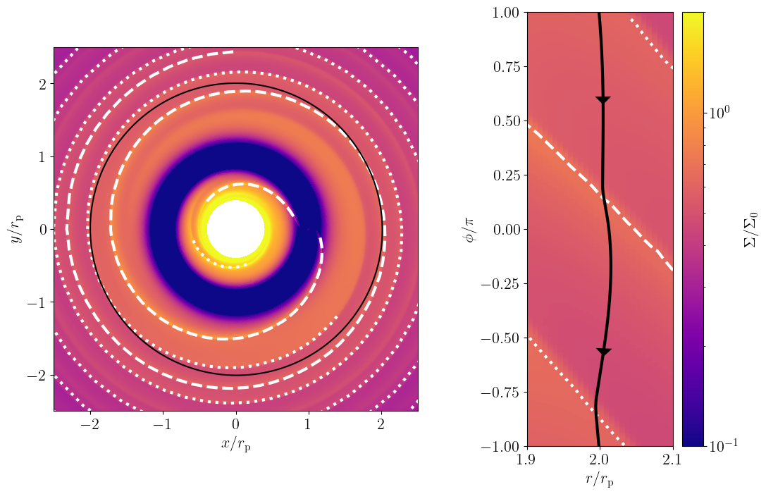
We begin by presenting the results from the fiducial run (RUN 1) to illustrate our shock wave analysis. The left panel of figure 1 shows a snapshot of the 2D gas surface density profile in the quasi-steady state ($t=1000$ planetary orbits) from RUN 1. The planet creates a deep disk gap in its vicinity ($r\sim 0.8$–$1.2r_{\rm p}$). The planet also excites spiral waves both interior to and exterior to its orbit. As discussed in previous studies (Zhu et al., 2015; Fung & Dong, 2015; Bae et al., 2017; Bae & Zhu, 2018), a planet excites more than one spiral arm in both the inner and outer disks. Following the previous studies, we refer to the arms directly attached to the planet as the primary arms and to the strongest arms that do not connect to the planet as the secondary arms. In the left panel of figure 1, the primary and secondary arms are marked by the dashed and dotted lines, respectively.

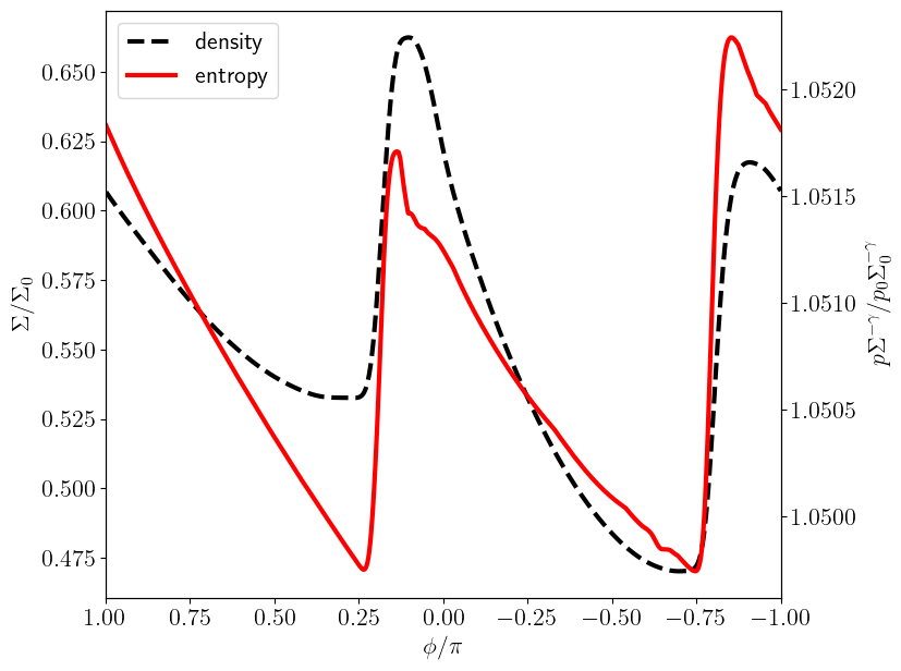
As described in section 2.3, we draw streamlines at different orbits and measure the entropy jumps across the arms. The black line in the left panel of figure 1 shows the streamline passing through the point $(r,\phi)=(2r_{\mathrm{p}},0)$ in this snapshot (see also the zoom-in of the vicinity of the streamline in the right panel of figure 1). Because the system has already reached a quasi-steady state, the streamlines on this snapshot approximately follow the trajectories of gas fluid elements. Figure 2 shows how the gas surface density and entropy of a fluid element along this streamline vary in the direction of the flow in the planet’s rest frame (negative $\phi$). The surface density of the element abruptly increases at the shock due to shock compression and then returns to the background value due to expansion. The entropy also increases at the shocks due to shock dissipation and then decreases due to cooling relaxation (the $Q_{\rm relax}$ term in equation (5)). After shock crossing, the change in entropy of the moving parcel decays on the timescale of $\sim t_{c}$, which is approximately 100 times the local Keplerian time. A close inspection of figure 2 shows that the measured entropy profile exhibits a small bump at $\phi\sim 0.1\pi$. This is a numerical artifact that arises when the streamline crosses a radial cell boundary and enters an adjacent outer cell with slightly higher entropy. However, this artificial bump does not affect our measurement of the entropy jump at the primary arm’s shock, located at $\phi/\pi\sim 0.2$.

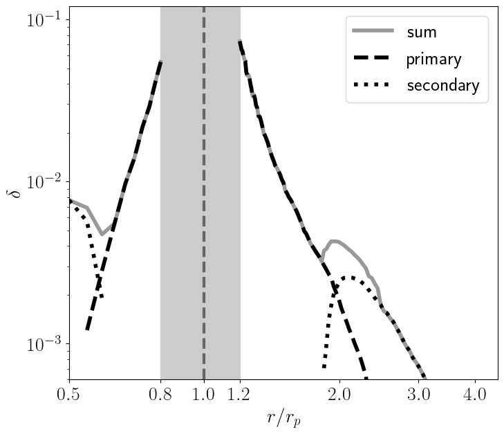
The streamline analysis illustrated above provides the dimensionless specific entropy jumps $\delta$ (equation (16)) at the primary and secondary shocks at different $r$, except in the gapped region $0.8<r/r_{\rm p}<1.2$, which is excluded from the analysis. These values are plotted in figure 3 as a function of $r$. The primary inner and outer arms yield a non-zero $\delta$ at $r/r_{\rm p}=0.8$ and 1.2, respectively, implying that both have already developed into shocks before propagating out of the gapped region. In contrast, the secondary inner and outer arms exhibit detectable entropy jumps at $r/r_{\rm p}\lesssim 0.7$ and $\gtrsim 2.0$, respectively, indicating that the secondary arms form shocks only after traveling considerable distances away from the planet. Interestingly, at large $|r-r_{\rm p}|$, the $\delta$ values of the secondary shocks surpass those of the primary shocks, meaning that disk heating by the secondary arms dominates over that by the primary ones. This is because the secondary arms have not experienced dissipation until they form shocks. The potential significance of the secondary shocks in disk heating is further discussed in section 4.1.

In the log–log plot of $\delta$ versus $r$ (figure 3), the radial profiles of $\delta$ for the inner and outer primary shocks appear as straight lines. This indicates that both approximately follow power laws. The same holds true for the fully developed secondary outer shock at $r/r_{\rm p}>2$. We cannot confirm such a trend for the secondary inner shock because the inner computational domain is too narrow for the secondary shock to fully develop. We provide empirical formulas for the entropy jumps in section 3.3.

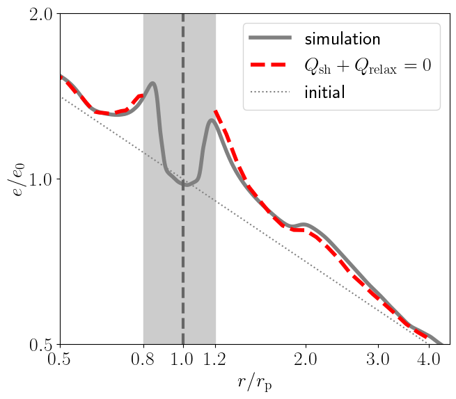
Before proceeding to a parameter study, we verify that the entropy jumps produced by the spiral shocks indeed cause disk heating, as predicted by equation (18). Figure 4 shows the radial profile of the azimuthally averaged specific internal energy from RUN 1 in the quasi-steady state. We expect that this internal energy profile is determined by the balance between shock heating and $\beta$ thermal relaxation (note that our simulations do not include viscous heating from Keplerian shear). Solving the thermal equilibrium equation $Q_{\rm sh}+Q_{\rm relax}=0$ for $e$, the internal energy profile in the steady state is predicted as

$$e_{\rm equil}=e_{\rm i}\left(1-\frac{\beta|1-\Omega_{\rm p}/\Omega(r)|}{2\pi}\delta\right)^{-1}.$$

(19)

We calculate $e_{\rm equil}$ using the radial $\delta$ profile obtained from the streamline analysis presented above. The result is overplotted in figure 4. We find that $e_{\rm equil}$ reproduces the azimuthally averaged $e$ in the steady state to within an accuracy of $\approx 5$%.

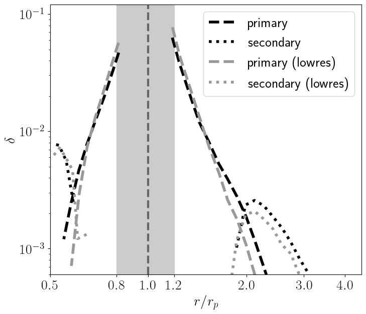
We also briefly examine the impact of numerical resolution on our measurements of entropy jumps. Here, we use a low-resolution version of RUN 1, with $448\times 792$ cells, resulting in half the resolution in both the radial and azimuthal directions. Figure 5 compares the radial profiles of $\delta$ for the primary and secondary arms from the low-resolution simulation with those from RUN 1 at standard resolution ($896\times 1584$ cells). We find that the low-resolution run reproduces the $\delta$ values for relatively large jumps ($\delta\gtrsim 0.005$) within 20% accuracy. The low-resolution run underestimates the smaller entropy jump at the secondary outer arm, but the error remains within $\approx$ 30%. Based on these comparisons, we expect that the simulations presented in this study produce $\delta$ values with a resolution-related error of less than 20–30%.

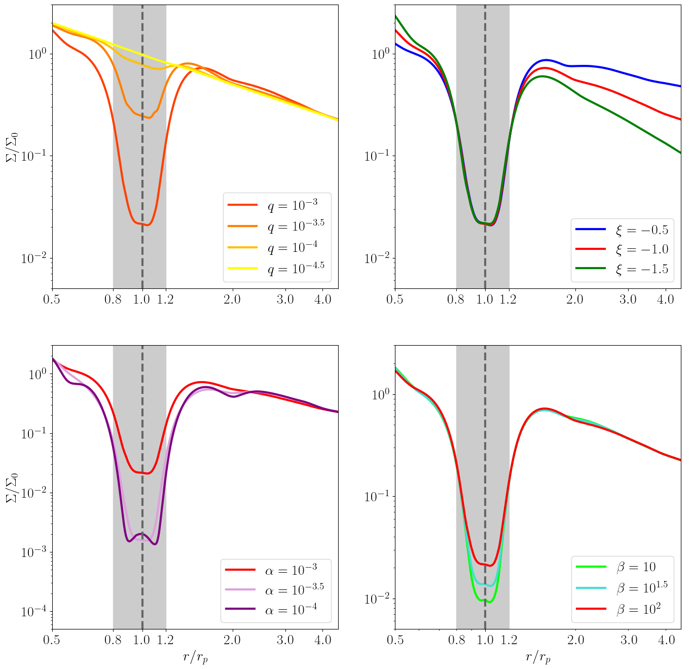
We now explore how our simulation results depend on the model parameters. Figure 6 shows the radial profiles of the azimuthally averaged surface density in the quasi-steady state from RUNs 1–10. It can be seen that different values of the planet mass $q$, surface density slope $\xi$, viscosity parameter $\alpha$, and thermal relaxation rate $\beta$ result in varying surface density profiles. However, as we will see below, the radial profiles of the entropy jumps at the spiral shocks are surprisingly similar among the models when scaled properly.

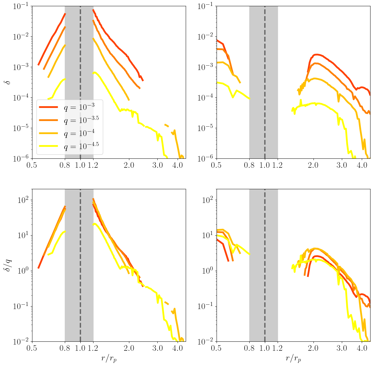
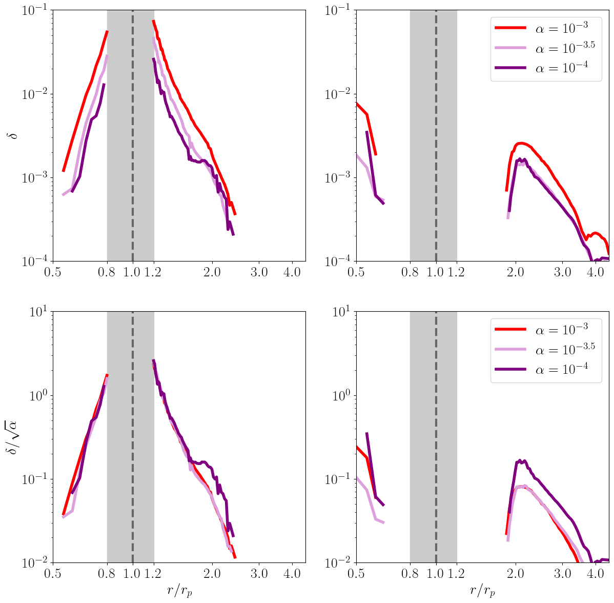
The upper left and right panels of figure 7 show the radial profiles of $\delta$ for the primary and secondary arms, respectively, from runs with different planet masses (RUNs 1 and 4–6). Their behavior is qualitatively similar to that observed in RUN 1 (see the previous subsection). Specifically, regardless of the planet’s mass, the $\delta$ values of the primary arms outside the gap region decreases monotonically with increasing $|r-r_{\rm p}|$, while the $\delta$ values of the secondary arms peak after traveling some distance from the planet. Once the secondary shock fully develops, its $\delta$ value exceeds that of the primary shock at the same location. The only significant difference is that the magnitude of $\delta$ scales approximately linearly with $q$. To see this, in the lower panels of figure 7, we plot the entropy jumps normalized by the planetary mass, $\delta/q$, as a function of $r$ from the four runs. We observe that the radial profiles of the normalized entropy jump almost coincide, particularly in the cases of $q=10^{-4}$–$10^{-3}$. The trend shifts slightly in the lowest-mass case of $q=10^{-4.5}$, potentially because the shocks for this case are too weak to resolve accurately.

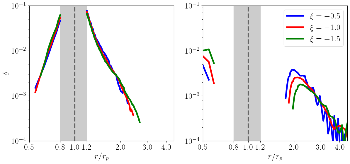
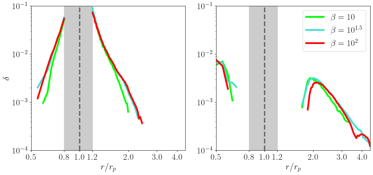
Figure 8 shows the radial profiles of $\delta$ for the primary and secondary arms from runs with different values of $\xi$ (RUNs 1–3). The $\delta$ profile for the primary arms is nearly independent of $\xi$, despite the background surface density profile depending on $\xi$. The same applies to the $\delta$ profile for the secondary arms. The only notable trend is that the location where the secondary arms form a shock (i.e., where $\delta$ becomes detectable) depends slightly on $\xi$. Specifically, as $\xi$ decreases, the shock formation position for the inner secondary arm shifts closer to the planet, while for the outer arm, it shifts farther. This dependence on $\xi$ likely reflects the initial radial sound velocity profile, $c_{i}\propto r^{-\xi-3/4}$ (see equation (8)). As $\xi$ decreases, the sound speed at $r<r_{\rm p}$ ($r>r_{\rm p}$) decreases (increases), causing the secondary arm to form a shock after traveling a shorter (longer) distance from the planet.

The upper panels of figure 9 show the same as figure 8 but from runs with different values of $\alpha$ (RUNs 1, 7, and 8). In most cases, $\delta$ crudely scales as $\sqrt{\alpha}$, as demonstrated in the lower panels of figure 9. This indicates that $\delta$ from our simulations depends weakly on the assumed viscosity. A notable exception is the secondary shock for $\alpha=10^{-4}$, whose $\delta$ profile approximately follows that of the secondary shock for $\alpha=10^{-3.5}$.

Figure 10 shows that varying $\beta$ over $10\leq\beta\leq 10^{2}$ has little effect on $\delta$. We note only that the peak of the $\delta$ distribution for the secondary outer arm shifts slightly outward as we vary $\beta$ from $10^{1.5}$ to $10^{2}$. This shift occurs because a higher $\beta$ results in an overall hotter disk with a higher sound speed, causing the secondary arm to form a shock farther from the planet.

In the previous subsection, we have observed that $\delta$ for the primary and secondary arms follows universal relations that only depend on $q$, $\alpha$, and $r/r_{\rm p}$. Here, we provide empirical formulas for the universal relations.

For the primary arms, we assume that $\delta$ takes the power-law form

$$\delta=10^{f_{0}}q\sqrt{\alpha}\cdot|r/r_{\mathrm{p}}|^{f_{1}},$$

(20)

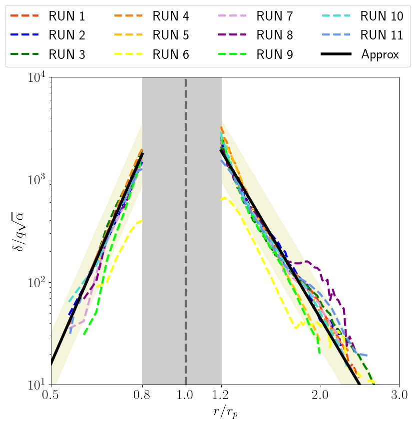
where $f_{0}$ and $f_{1}$ are fitting parameters. We searched for the set of $(f_{0},f_{1})$ that best reproduces the $\delta$ profiles for each of the primary inner and outer arms, using the data from all runs except for the lowest planet mass case (RUN 6; $q=10^{-4.5}$) and the low viscosity case (RUN 8; $\alpha=10^{-4}$), which appear to be slightly out of trend. The obtained best-fit parameters for the primary inner and outer arms are $(f_{0},f_{1})=(4.22,10.02)$ and $(f_{0},f_{1})=(3.87,-7.37)$, respectively. Figure 11 demonstrates that the best-fit formulas reproduce the results form all runs except RUNs 6 and 8 to within a factor of 2. Assuming radiative equilibrium where $Q_{\rm sh}\propto\sigma T^{4}$, with $\sigma$ being the Stefan–Boltzmann constant, a factor of 2 error in $\delta$ translates into an approximately 20% error in the disk interior temperature $T$. For RUNs 6 and 8, our empirical formulas are less accurate, with a relative error of up to a factor of 3. The smaller-than-expected entropy jumps observed in RUN 6 are potentially due to the inefficient nonlinearity of the planet-induced waves, i.e., $q<q_{\rm th}$, in this run (see section 2.4). We note that the resolution-related errors in the measured $\delta$ values are less than 20–30% (see section 3.1) and are therefore smaller than the errors arising from the fitting.

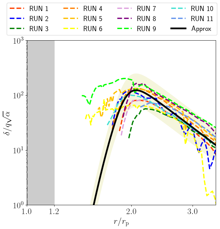
We also provide an empirical formula for $\delta$ for the secondary outer arm, which has been found to fully develop into a shock within our computational domain. We assume that the secondary arm’s $\delta$ also follows the form given by (20) but with a cutoff at small $|r-r_{\rm p}|$. By fitting our simulation results, we find that $\delta$ for the secondary outer arm scales as $r^{-4.79}$ at large radial distances. We propose the formula

$$\delta=10^{3.7}q\sqrt{\alpha}\biggl{(}\dfrac{r}{r_{\mathrm{p}}}\biggr{)}^{-4.79}\left[\biggl{(}\dfrac{r/r_{\mathrm{p}}-1}{0.95}\biggr{)}^{-12}+1\right]^{-1},$$

(21)

where the last factor represents the cutoff. This formula reproduces our simulation results to within a factor of a few (figure 12).

As noted in section 2.1, our simulations do not include viscous heating from the disk’s Keplerian shear. In reality, however, both Keplerian shear and planet-induced shocks contribute to disk heating. Here, we use the analytic expressions for the specific entropy jump $\delta$ obtained in this study to predict when and where shock heating may dominate over viscous heating.

The viscous heating rate is given by (Lynden-Bell & Pringle, 1974; Pringle, 1981)

$$Q_{\rm vis}=\frac{9}{4}\nu\Sigma\Omega_{\rm K}^{2}=\frac{9(\gamma-1)}{4}\alpha\Sigma e\Omega_{\rm K}.$$

(22)

The ratio between the shock heating rate $Q_{\rm sh}$ (equation (18)) and $Q_{\rm vis}$ can be written as

	$\displaystyle\frac{Q_{\rm sh}}{Q_{\rm vis}}$	$\displaystyle=$	$\displaystyle\frac{2}{9\pi(\gamma-1)}\left|1-\frac{\Omega_{\rm p}}{\Omega_{\rm K}(r)}\right|\frac{\delta}{\alpha}$		(23)
		$\displaystyle\approx$	$\displaystyle 0.18\left|1-\left(\frac{r}{r_{\rm p}}\right)^{3/2}\right|\frac{\delta}{\alpha}.$

Notably, the ratio depends only on $r/r_{\rm p}$ and $\delta/\alpha$. Furthermore, except at $r\gg r_{\rm p}$, the ratio is determined solely by $\delta/\alpha$.

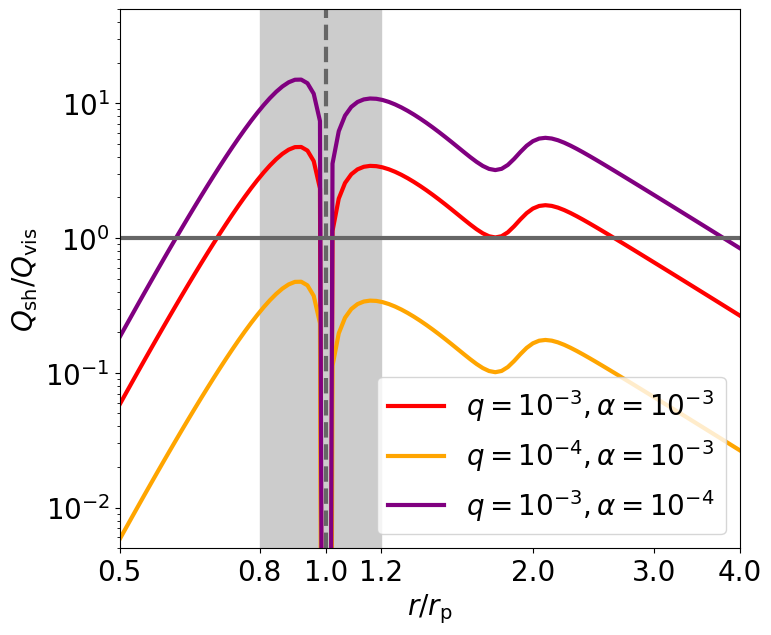
Our empirically obtained relation $\delta\propto q\sqrt{\alpha}$ suggests that the heating rate ratio $Q_{\mathrm{sh}}/Q_{\mathrm{vis}}$ scales as $q/\sqrt{\alpha}$. Figure 13 illustrates the radial distribution of $Q_{\mathrm{sh}}/Q_{\mathrm{vis}}$ for $q=10^{-4}$ and $10^{-3}$. Here, the shock heating rate accounts for the contributions from the primary inner and outer arms, as well as the secondary outer arm (equations (11) and (12), respectively). We find that shock heating by a planet with mass $q=10^{-3}$ can overwhelm viscous heating if $\alpha<10^{-3}$. Our result aligns with the findings by Ziampras et al. (2020), who showed that the shocks induced by a Jupiter-mass planet orbiting a solar-mass star ($q\approx 10^{-3}$) significantly heat a disk with $\alpha=10^{-3}$ (see their figure 6).

It is worth pointing out that the secondary outer shock produces a bump in $Q_{\rm sh}/Q_{\rm vis}$ at $r\approx 2r_{\rm p}$. This bump is large enough for $Q_{\rm sh}$ to exceed $Q_{\rm vis}$ in the case of $q=10^{-3}$ and $\alpha=10^{-4}$. This suggests that the secondary arms may have a non-negligible impact on the disk’s thermal structure away from the planetary orbit. This effect warrants further investigation in future hydrodynamical simulations with wider radial computational domains.

We have demonstrated that shock heating by planet-induced spiral arms may serve as an important heating source for the disk harboring the planet. However, our simulations have two important limitations that should be addressed in future work. Firstly, the computational domain employed in our simulations only covers $r>0.5r_{\rm p}$ due to computational cost. As a result, we could not fully observe how the secondary inner arm develops into a shock. Meanwhile, we have seen that the heating by the fully developed secondary outer shock can dominate over that by the primary outer shock, when compared at the same orbital radius. This is likely the case for the inner shocks as well, since we observe that the secondary shock’s $\delta$ exceeds that of the primary shock already at the inner boundary of our computational domain (see, e.g., figure 3). Simulations with an extended inner computational domain, down to $r\sim 0.25r_{\rm p}$, will allow us to confirm this expectation. Previous studies (Zhu et al., 2015; Bae et al., 2017) already showed that the tertiary inner arm can also emerge at $r\lesssim 0.5r_{\rm p}$. Shock heating by this tertiary arm may potentially dominate over that by the secondary arm at large distances from the planet.

Secondly, our simulation models are 2D and therefore neglect any effects arising from the vertical structure of the disk and spiral arms. The spiral shocks can be weaker in 3D disks, where the shocked gas is allowed to expand vertically, leading to adiabatic cooling (Bate et al., 2003; Boley & Durisen, 2006; Lyra et al., 2016). Therefore, our 2D simulations could overestimate the magnitude of $\delta$. Nevertheless, it is possible that the scaling of $\delta$ with the model parameters and $r$ found in this study also holds in 3D disks. If this is the case, our 2D approximation would primarily affect the numerical prefactors in our empirical formulas for $\delta$, equations (20) and (21). In any case, 3D simulations will be necessary to validate our empirical formulas quantitatively.

The simple $\beta$-relaxation prescription employed in this study may affect our disk’s thermal structure. However, we expect that this treatment primarily influences disk cooling and does not significantly impact the shock heating rate. In fact, our simulations show that varying the dimensionless thermal relaxation timescale $\beta$ over the range $10\leq\beta\leq 10^{2.5}$ has little effect on $\delta$ (see figure 10), indicating that the shock heating strength is insensitive to the thermal relaxation process as long as the relaxation timescale is much longer than the local orbital timescale. For smaller $\beta$ ($\sim 0.01$–$1$), radiative damping of planet-induced spiral shocks (Miranda & Rafikov, 2020) could affect $\delta$ profiles. However, we have not explored this parameter range as shock heating would have little impact on disk temperature in such rapidly cooling disks.

References

- Andrews (2020) Andrews, S. M. 2020, ARA&A, 58, 483â528
- Bae et al. (2023) Bae, J., Isella, A., Zhu, Z., et al. 2023, in Astronomical Society of the Pacific Conference Series, Vol. 534, Astronomical Society of the Pacific Conference Series, ed. S. Inutsuka, Y. Aikawa, T. Muto, K. Tomida, & M. Tamura, 423
- Bae & Zhu (2018) Bae, J., & Zhu, Z. 2018, ApJ, 859, 118
- Bae et al. (2017) Bae, J., Zhu, Z., & Hartmann, L. 2017, ApJ, 850, 201
- Bate et al. (2003) Bate, M. R., Lubow, S. H., Ogilvie, G. I., & Miller, K. A. 2003, MNRAS, 341, 213
- Bitsch et al. (2015) Bitsch, B., Johansen, A., Lambrechts, M., & Morbidelli, A. 2015, A&A, 575, A28
- Bitsch et al. (2019) Bitsch, B., Raymond, S. N., & Izidoro, A. 2019, A&A, 624, A109
- Boley & Durisen (2006) Boley, A. C., & Durisen, R. H. 2006, ApJ, 641, 534
- Brown & Ogilvie (2024) Brown, J. J., & Ogilvie, G. I. 2024, MNRAS, 534, 39
- Delage et al. (2023) Delage, T. N., Gárate, M., Okuzumi, S., et al. 2023, A&A, 674, A190
- Fukuhara & Okuzumi (2024) Fukuhara, Y., & Okuzumi, S. 2024, PASJ, 76, 708
- Fung & Dong (2015) Fung, J., & Dong, R. 2015, ApJ, 815, L21
- Gammie (2001) Gammie, C. F. 2001, ApJ, 553, 174
- Goldreich & Tremaine (1979) Goldreich, P., & Tremaine, S. 1979, ApJ, 233, 857
- Goodman & Rafikov (2001) Goodman, J., & Rafikov, R. R. 2001, ApJ, 552, 793
- Johansen et al. (2021) Johansen, A., Ronnet, T., Bizzarro, M., et al. 2021, Science Advances, 7, eabc0444
- Kleine et al. (2020) Kleine, T., Budde, G., Burkhardt, C., et al. 2020, Space Sci. Rev., 216, 55
- Kondo et al. (2023) Kondo, K., Okuzumi, S., & Mori, S. 2023, ApJ, 949, 119
- Kruijer et al. (2020) Kruijer, T. S., Kleine, T., & Borg, L. E. 2020, Nature Astronomy, 4, 32
- Lichtenberg et al. (2019) Lichtenberg, T., Golabek, G. J., Burn, R., et al. 2019, Nature Astronomy, 3, 307
- Lin & Papaloizou (1993) Lin, D. N. C., & Papaloizou, J. C. B. 1993, in Protostars and Planets III, ed. E. H. Levy & J. I. Lunine, 749
- Lynden-Bell & Pringle (1974) Lynden-Bell, D., & Pringle, J. E. 1974, MNRAS, 168, 603
- Lyra et al. (2016) Lyra, W., Richert, A. J. W., Boley, A., et al. 2016, ApJ, 817, 102
- Masset (2000) Masset, F. 2000, A&AS, 141, 165
- Miranda & Rafikov (2020) Miranda, R., & Rafikov, R. R. 2020, ApJ, 892, 65
- Mori et al. (2021) Mori, S., Okuzumi, S., Kunitomo, M., & Bai, X.-N. 2021, ApJ, 916, 72
- Müller et al. (2012) Müller, T. W. A., Kley, W., & Meru, F. 2012, A&A, 541, A123
- Oka et al. (2011) Oka, A., Nakamoto, T., & Ida, S. 2011, ApJ, 738, 141
- Pringle (1981) Pringle, J. E. 1981, ARA&A, 19, 137
- Rafikov (2002) Rafikov, R. R. 2002, ApJ, 569, 997
- Rafikov (2016) Rafikov, R. R. 2016, ApJ, 831, 122
- Richert et al. (2015) Richert, A. J. W., Lyra, W., Boley, A., Mac Low, M.-M., & Turner, N. 2015, ApJ, 804, 95
- Sato et al. (2016) Sato, T., Okuzumi, S., & Ida, S. 2016, A&A, 589, A15
- Shakura & Sunyaev (1973) Shakura, N. I., & Sunyaev, R. A. 1973, A&A, 500, 33
- Stone et al. (2020) Stone, J. M., Tomida, K., White, C. J., & Felker, K. G. 2020, ApJS, 249, 4
- Val-Borro et al. (2006) Val-Borro, M. D., Edgar, R. G., Artymowicz, P., et al. 2006, MNRAS, 370, 529
- Zhu et al. (2015) Zhu, Z., Dong, R., Stone, J. M., & Rafikov, R. R. 2015, ApJ, 813, 88
- Ziampras et al. (2020) Ziampras, A., Ataiee, S., Kley, W., Dullemond, C. P., & Baruteau, C. 2020, A&A, 633, A29