Modeling measurements for quantitative imaging subsurface targets ††thanks: This work was supported by the AFOSR Grant FA9550-24-1-0191. A. D. Kim also acknowledges support by NSF Grant DMS-1840265.
Abstract
We study ground-penetrating synthetic aperture radar measurements of scattering by targets located below a rough air-soil interface. By considering the inherent space/angle limitations of this imaging modality, we introduce a simplified model for measurements. This model assumes (i) first-order interactions between the target and the air-soil interface, (ii) scattering by the target below a flat air-soil interface, and (iii) a point target model. Using the method of fundamental solutions to simulate two-dimensional simulations of scalar waves for the direct scattering problem, we systematically study each of these data modeling assumptions. To test and validate these assumptions, we apply principal component analysis to approximately remove ground bounce signals from measurements and then apply Kirchhoff migration on that processed data to produce images. We show that images using this modeled data are nearly identical to those that use simulated measurements from the full direct scattering problem. In that way, we show that this model contains the essential information contained in measurements. Consequently, it provides a theoretical framework for understanding how inherent space/angle limitations affect subsurface imaging systems.
Index Terms:
Ground-penetrating synthetic aperture radar, subsurface imaging, rough surface, modelingThis work has been submitted to the IEEE for possible publication. Copyright may be transferred without notice, after which this version may no longer be accessible.
I Introduction
Landmines pose a serious issue for humanity as they remain dangerous for decades after their deployment, killing and injuring civilians and rendering the land inaccessible. The economic burden of landmines is huge, especially for developing countries [1]. It is therefore crucially important to develop safe and robust methods for detection of buried landmines, so that they may be subsequently removed.
To locate landmines safely, non-touch-based sensors such as ground penetrating radar (GPR) or metal detectors are preferable [2]. GPR can detect both metal and plastic landmines and its weight is light so that it can be mounted on a unmanned aerial vehicle (UAV) allowing for safe inspection flying above the air-soil interface as proposed in [3, 4, 5]. It is this UAV configuration that we consider here. Specifically, we consider a sequence of measurements taken a various locations along a prescribed flight path making up a synthetic aperture, which we call ground-penetrating synthetic aperture radar (GP-SAR).
Using UAVs to acquire GP-SAR measurements allows for flight paths at relatively low elevations above air-soil interfaces. These low-elevation flight paths help to mitigate environmental factors that would introduce strong position, navigation, and timing noises [3]. Assuming that buried landmines are spaced apart relatively far from one another (meters) compared to the central wavelength used in the imaging system (centimeters), we consider using relatively short flight paths for relatively small, site-specific imaging regions. Shorter flight paths imply fewer measurements which, in turn, require less data storage and faster processing. These factors may yield efficiency gains through relieving the communication burden by the UAV, for example. The UAV may repeatedly apply this rapid site-specific method to cover larger regions.
There are several challenges in this problem. For example, the air-soil interface is generally not flat and is unknown. The electromagnetic properties of soil vary widely. They may include dispersion and absoprtion, for example, and are generally unknown. Potential subsurface targets also vary widely in shape, size, and electromagnetic properties. Measurements of signals scattered by subsurface targets involve complex scattering by the rough air-soil interface, the subsurface targets, and the multiple interactions between them. Various factors of uncertainty always lead to noisy measurements.
In this work, we seek to determine a model for GP-SAR measurements to be used for subsurface imaging. We aim to have this model strike a balance between the complexities of the problem discussed above and the limitations inherent in this imaging modality. Additionally, we want this model to be easily extensible to include more sophistication, as needed.
We determine a GP-SAR measurement model by systematically testing and validating a sequence of assumptions within the context of a specific imaging method. This imaging method first uses principal component analysis (PCA) to approximately remove ground bounce signals, and then applies Kirchhoff migration (KM) on that processed data to produce an image that identifies and locates subsurface targets. The electromagnetic properties of soil need not be known to apply PCA for ground bounce removal. However, we assume here that the ground permittivity is known for KM.
We start with a direct scattering problem in which a subsurface target is situated below a rough air-soil interface. We assume that the size of the target and the depth below the air-soil interface where it is situated are on the order of centimeters and therefore comparable to the central wavelength. We limit our attention here to two-dimensional scalar wave propagation where the soil and target are characterized by their respective relative dielectric constants. Despite these simplifications, this problem includes strong scattering by the rough air-soil interface, and multiple scattering interactions between the target and this interface. These interactions are the crucially important physical factors affecting measured signals in this problem which make this imaging problem especially challenging. Additionally, we include additive measurement noise in measurements.
The GP-SAR imaging problem is a severely limited aperture imaging problem. Because of the inherent space/angle limitations in GP-SAR measurements, we find that the imaging method we use here produces an image with limited spatial information about the target – essentially, images only show a representative single point. It is most likely that any imaging method will behave similarly because of these inherent limitations in measurements. In light of these results, we consider the following sequence of simplifying assumptions:
-
(i)
First-order interactions between the target and air-soil interface
-
(ii)
Flat air-soil interface approximation for scattering by the target
-
(iii)
A point target model
In this paper, we systematically test and validate each of these assumptions in sequence and show that the images resulting from approximating measurements with them closely match those using the solution of the full direct scattering problem. From these results, we are able to propose a simplified model for measurements. This simplified model immediately provides valuable insight into how the imaging method we use here works. Moreover, this simplified model provides a theoretical framework on which one may naturally introduce extensions for more complex imaging problems.
The remainder of the paper is as follows. In Section II we discuss the boundary value problem for the direct scattering problem we study here. In Section III we discuss the method of fundamental solutions which we use to solve this direct scattering problem. We give the details of the imaging method we use here to evaluate approximations in Section IV. Our main results are given in Section V where we systematically introduce, test, and validate the three simplifying assumptions leading to the determination of the measurement model. We give our conclusions in Section VI.
II The direct scattering problem
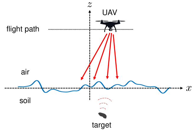
A sketch of the physical problem is illustrated in Fig. 1. As a UAV travels along its flight path, it emits a multi-frequency signal that propagates down towards the air-soil interface. Part of this signal is reflected by the air-soil interface and the other part penetrates into soil. The part of the signal that has penetrated into the soil is then scattered by a subsurface target and the part of this scattered signal that transmits back across the air-soil interface into air is subsequently recorded by a receiver on the UAV. In this work, we assume the start-stop approximation which neglects the motion of the UAV between emission and reception of each measurement along the flight path. Doing so allows us to focus our discussion on the problem for a fixed source location at a fixed frequency since measurements consist of repeated solution of this problem for different source locations and frequencies.
We describe the boundary value problem governing scalar wave scattering by a target located below an air-soil interface. Let denote this air-soil interface. Below this air-soil interface is a target occupying region with boundary . We define the following three regions.
-
•
Region 0 (air)
-
•
Region 1 (soil exterior to the target)
-
•
Region 2 (interior to the target)
We consider the medium in each of these three regions to be uniform so that each is characterized solely by their respective wavenumbers: in Region 0, in Region 1, and in Region 2. Here, is the circular frequency, is the wavespeed, and and are the relative dielectric constants for the soil and the target, respectively.
Let denote the scattered field in Region . These fields satisfy
| (1a) | |||||
| (1b) | |||||
| (1c) | |||||
with denoting the Laplacian. The incident field in Region 0 is the free-space Green’s function (in air) centered at position , which we denote by . We supplement these equations above by boundary conditions. On (the air-soil interface), we require
| (2) |
with denoting the normal derivative for the air-soil interface. On (the target boundary), we require
| (3) |
with denoting the normal derivative for the target boundary. Additionally, we require appropriate outgoing conditions for all of these scattered fields.
III The method of fundamental solutions
To solve the system consisting of (1a), (1b), and (1c) subject to (2), (3), and outgoing coniditions, we use the method of fundamental solutions (MFS). This method was introduced by Mathon and Johnston [6]. It provides an accurate and efficient computational method for solving the full scattering problem. The text by Wriedt et al [7] provides an overview of this method and its applications to various problems. A recent review paper by Cheng and Hong [8] focuses on solvability, uniqueness, convergence and stability of the MFS.
This method most closely resembles integral equation methods, but is simpler to understand and implement. Just like integral equation methods, the MFS is a so-called meshless method in that it does not rely on an underlying mesh over the domain. We have successfully applied the MFS to multiple scattering problems involving randomly oriented ellipsoids in an uniform and unbounded medium [9]. To our knowledge, the application of MFS to solve the direct scattering problem here with a rough air-soil interface has not been done.
The key idea behind the MFS is to introduce approximations for the scattered fields: , , and , that exactly solve (1a), (1b), and (1c), respectively. These approximations are superpositions of finitely-many fundamental solutions (free-space Green’s functions) whose source positions lie outside of the region. Because their source points lie outside of the region, the evaluation of these fundamental solutions within the region exactly solve the differential equation. Moreover, since each of those fundamental solutions satisfies the appropriate outgoing conditions, so does their superposition and hence, so do the MFS approximations. We determine the relative weighting of each individual fundamental solution by a collocation method for the boundary conditions. Thus, the MFS approximation exactly solves the differential equation and approximately satisfies the boundary conditions through what is tauntamount to an interpolation procedure. Because of this, the MFS is able to obtain spectral accuracy uniformly throughout the domain.
The underlying challenge in using the MFS lies in choosing the positions for the source points. Typically, they are chosen to attempt to sample uniformly the boundary/interface but are placed slightly away from it and outside of the region. There is a natural relationship between the distance away from the boundary/interface where source points are placed, the conditioning of the resulting linear system to determine the weights of the superposition of fundamental solutions, and the accuracy of the resulting approximation. When those source points are closer to the boundary/interface, the resulting linear system is more diagonally dominant leading to better conditioning, but the approximation is less accurate. On the other hand, the farther away those source points are from the boundary/interface, the smoother the approximation is leading to higher accuracy, but with worse conditioning. There is some theory on the optimal placement of source points [10], but that is limited to two-dimensional problems.
In what follows, we describe our implementation of the MFS for the direct scattering problem consisting of (1a), (1b), and (1c) subject to (2), (3), and outgoing conditions. We limit this discussion to scattering in the two-dimensional -plane. Extending this method to three-dimensional problems is straight-forward in principle, but requires additional considerations for efficient solution which we do not address here.
III-A MFS approximations
In two dimensions, the air-soil interface is . Let for denote a grid of points that uniformly samples the interval with meshwidth . We then use the points for to sample the air-soil interface. At we use as the unit normal to this air-soil interface, . Note that this choice always points into Region 0.
We assume the target boundary is a closed curve that can be parameterized according to for with . Let for denote a grid of points that uniformly samples with meshwidth . We then use the points for to sample the target boundary. At we use as the unit normal to this target boundary, . Note that this choice always points into Region 1.
We introduce two, user-defined parameters: and . The MFS approximation for scattered field in Region 0 is then
| (4) |
with denoting the free-space Green’s function with wavenumber and denoting any point in Region 0. Note that the source positions: for lie outside of Region 0 (inside Region 1), so (4) exactly solves (1a) in Region 0. The expansion coefficients for are to be determined.
The MFS approximation for scattered field in Region 1 is given by
| (5) |
with denoting the free-space Green’s function with wavenumber and denoting any point in Region 1. Note that the source points for and for lie outside of Region 1 (inside of Region 0 and Region 2, respectively), so (5) exactly solves (1b) in Region 1. The expansion coefficients for and for are to be determined.
Finally, the MFS approximation for the field interior to the target in Region 2 is
| (6) |
with denoting the free-space Green’s function with wavenumber and denoting any point in Region 2. Since the source points for lie outside of Region 2 (inside Region 1), (6) exactly solves (1c) in Region 2. The expansion coefficients for are to be determined.
MFS approximations (4), (5), and (6) are all just superpositions of free-space Green’s functions whose source positions lie outside of the regions where they are evaluated. Additionally, each of these free-space Green’s functions satisfy the correct outgoing conditions. Therefore, (4), (5), and (6) satisfy the appropriate outgoing conditions in their respective regions.
III-B Collocation method for boundary conditions
In (4), (5), and (6), there are undetermined coefficients: and for , and and for . To determine these undetermined expansion coefficients, we apply a collocation method for boundary conditions (2) and (3).
III-C MFS system
Let , , and be matrices whose entries are given by
| (11a) | ||||
| (11b) | ||||
| (11c) | ||||
| (11d) | ||||
Let and be the matrices whose entries are given by
| (12a) | ||||
| (12b) | ||||
Let and be the matrices whose entries are given by
| (13a) | ||||
| (13b) | ||||
Finally, let , , , and denote the matrices whose entries are given by
| (14a) | ||||
| (14b) | ||||
| (14c) | ||||
| (14d) | ||||
Because and , these matrix entries never correspond to evaluation of the free-space Green’s function where it is singular.
Using these matrices, we find that the equations given by (7), (8), (9), and (10) as the following block linear system,
| (15) |
Here, and are the -vectors whose components are and for , respectively, and and are the -vectors whose components are and for , respectively. The right-hand side is made up of -vectors and whose components are given by
| (16a) | ||||
| (16b) | ||||
for .
III-D Example
Block system (15) can be solved numerically leading to the determination of the coefficients in (4), (5), and (6). With those expansion coefficients determined, those approximations can be evaluated anywhere within the regions to which they are defined. Here, we show an example computation.
In Fig. 2 we show MFS results for the fields scattered due to a point source located at cm, at frequency GHz and with cm GHz. For soil, we have used and for the target we have used .
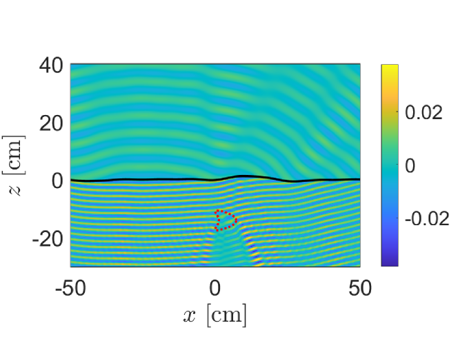
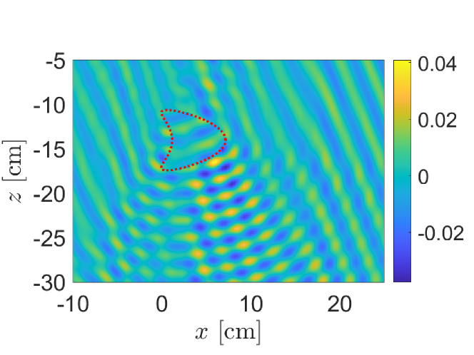
The air-soil interface is one realization of a Gaussian-correlated random rough surface with RMS height cm and correlation length cm generated using the method described by Tsang et al [11]. In Fig. 2, we have used cm and for the air-soil interface. For the target, we consider the “kite” whose boundary is given by and . We have set .
The example shown in Fig. 2 illustrates that the MFS approximation captures the complex interactions of the fields with the rough air-soil interface and the target. These complex interactions involve a variety of spatial scales and the computed solution smoothly transitions over these scales. Because the MFS is an easy to implement method and accurately accounts for the underlying physics of multiple scattering by the rough air-soil interface and the target, we use it for simulating measurements.
IV The inverse scattering problem
The objective for the inverse scattering problem is to reconstruct the subsurface target from GP-SAR measurements. That target is characterized completely by its “support” given by and its relative dielectric constant . The extent to which we can recover all or some of these characteristics depend on the information contained in measurements. For GP-SAR measurements, we identify inherent limitations that affect the solution of the inverse scattering problem.
IV-A GP-SAR measurements
GP-SAR measurements are multi-frequency signals taken over several locations along the flight path. Let for denote the frequencies used to sample the system bandwidth and let for denote the locations along the flight path where these multi-frequency signals are emitted and measured. For each location, we set and solve the direct scattering problem described above for frequency . We take as measurements evaluations of corresponding to the scattered field evaluated at frequency at position . Through repeated solution of the direct scattering problem over all frequencies and all source/measurement positions, we obtain the measurement matrix . Measurements are typically corrupted by additive noise, so we model the entries of the data matrix as the sum,
| (17) |
with denoting additive Gaussian white noise.
Note that we have considered only frequency-flat, isotropic point sources. Additionally, we use point-wise evaluations of the scattered field as measurements. Different sources and measurements can be used through an appropriate modification of the direct scattering problem. However, the measurement matrix we use here is fundamental in that other sources and measurements can be computed from it.
IV-B Principal component analysis for ground bounce removal
A key challenge in this inverse scattering problem is the ground bounce signals in the measurements. Ground bounce signals correspond to the portion of measurements that are reflections of the incident field by the air-soil interface. They contribute more to the overall power in measurements than signals scattered by the subsurface target. However, those signals carry little or no information about the target. Therefore, we must remove ground bounce signals from measurements to be able to image the subsurface target.
When the air-soil interface is known, one can model these reflections and use those to remove them from measurements. Otherwise, one needs to consider alternative methods. In what follows, we describe how to use principal component analysis (PCA) to approximately remove ground bounce signals from measurements.
For PCA, we first compute the singular value decomposition (SVD) of the data matrix so that where denotes the Hermitian (conjugate) transpose. We assume the non-zero singular values along the diagonal of are in descending order. The key idea with PCA is that ground bounce signals are stronger than the scattered signals, so they are associated with the largest singular values. Hence, we consider
| (18) |
instead of . Here, is a user-defined truncation, and are the th columns of and , respectively. Provided that is chosen well, the resulting processed data matrix is amenable to imaging methods such as Kirchhoff migration which we explain below.
Using PCA to approximately remove ground bounce signals is completely data-driven. It does not require a priori knowledge of the electromagnetic properties of soil. Rather, it is based off of the assumption that the ground bounce signals dominate the measurements over the scattered signals by the target.
IV-C Kirchhoff migration
Kirchhoff migration (KM), also known as back-propagation or reverse time-migration, is a so-called sampling method [12]. Rather than having to solve an optimization problem to reconstruct an image of the target, KM requires only the evaluation of an imaging function over some region of interest, which we call the imaging region. Let denote a point in this imaging region. The KM imaging function is given by
| (19) |
with denoting the entry of , denoting what we call the illuminations and denoting the complex conjugate.
To define the illuminations, we assume we know the mean elevation of the flight path over the air-soil interface. Additionally, we assume we know the relative refractive index for soil denoted by . Let , , and . The illuminations are given by
| (20) |
The illuminations given in (20) correspond to the phase accumulated from scattering by a point target at location below a flat air-soil interface on using the Fresnel approximation. Additionally, illuminations (20) assume only one interaction between this point target and the flat air-soil interface, whereas the full boundary value problem includes infinitely-many of these interactions.
We form an image by plotting over the imaging region. When KM is effective, this plot reveals spatial information about the target. Note that this implementation of KM starts with measurements defined by (17) which include additive measurement noise. We then compute (18), the processed data matrix resulting from PCA which approximately removes ground bounce signals. Finally, this KM implementation evaluates (19) with illuminations (20) defined for a flat air-soil interface.
In this formulation of KM, we assume a priori knowledge of a ground permittivity and the mean height of the flight path over the air-soil interface . Other than those two parameters, no other parameters are needed to evaluate (19).
IV-D Examples
We now show examples of images produced using the methods described above on data simulated using the MFS. For these examples, we have used frequencies uniformly sampling the bandwidth between GHz and GHz (at MHz steps) similarly to what was done by Garcia-Fernandez et al [4]. We have set the elevation above the mean of the air-soil interface to be cm and use spatial locations unformly sampling the synthetic aperture of size cm (at cm steps).
We consider the air-soil interface to be one realization of a Gaussian-correlated random rough surface with RMS height cm and correlation length cm. We showed recently that random rough surfaces with these parameters exhibit enhanced backscattering indicating significant multiple scattering caused by the surface roughness. As suggested by Daniels [13], we set for soil and for the target. For the MFS computations to generate simulated measurements, we used points to sample the surface over the interval of length cm.
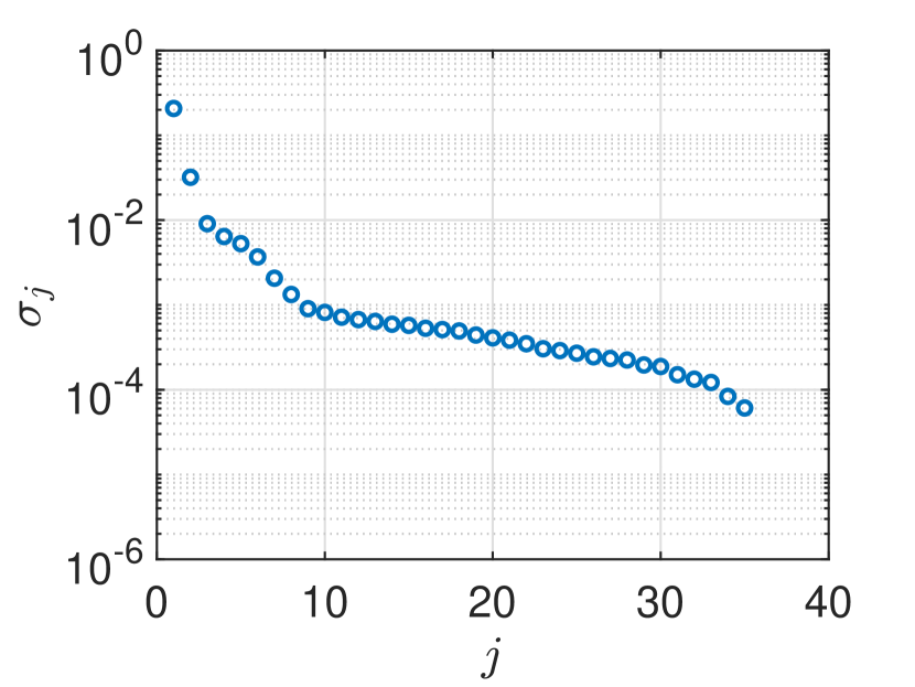
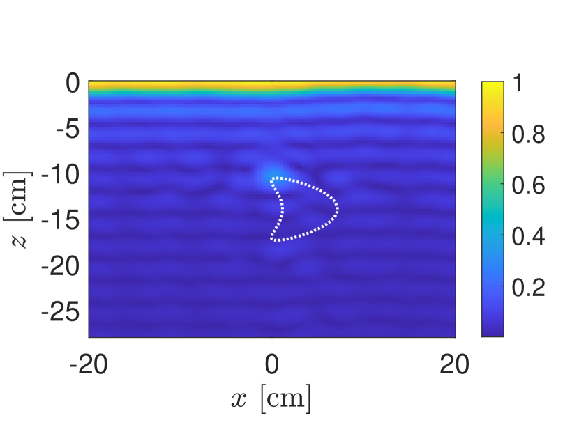
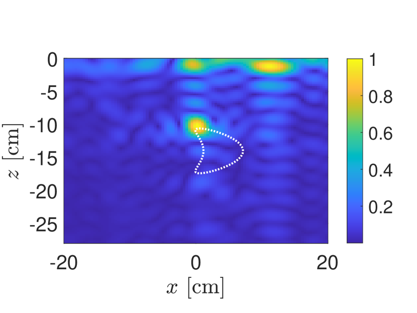
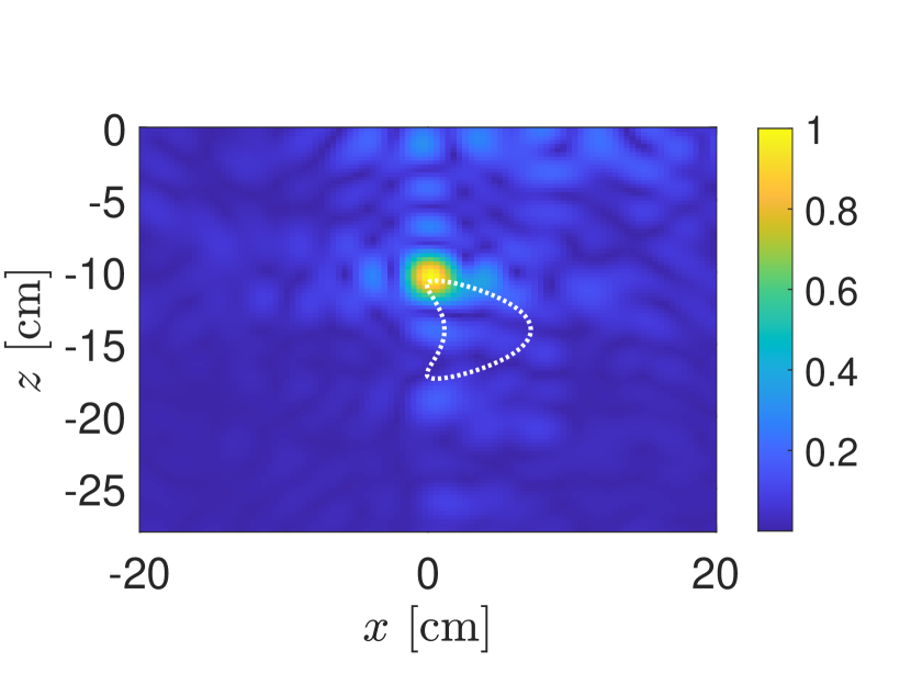
In Fig. 3 we show results for the same “kite” target used in Fig. 2. We have added measurement noise to the simulated measurements so that SNR dB. The singular values of the data matrix are shown in Fig. 3(a). We observe from those results that the first two singular values are significantly larger than the remaining singular values with large gaps between them. In Figs. 3(b)–(d) we show KM images applied to the original data matrix (Fig. 3(b)), the PCA processed data matrix with one term removed (Fig. 3(c)), and the PCA processed data matrix with two terms removed (Fig. 3(d)). These KM images show plots of the absolute value of (19) normalized by its maximum value.
These results show how PCA effectively removes the ground bounce signals that interfere with the identification and location of the target. In Fig. 3(b) we find that the image is concentrated near corresponding to the air-soil interface. With the contribution by the first singular value removed, the image shown in Fig. 3(c) identifies the target but also has artifacts located near the air-soil interface. After removing the contributions by the first two singular values, we find in Fig. 3(d) that the resulting image identifies the target. Specifically, it appears to identify the single point on the boundary of the target that is closest to the synthetic aperture.

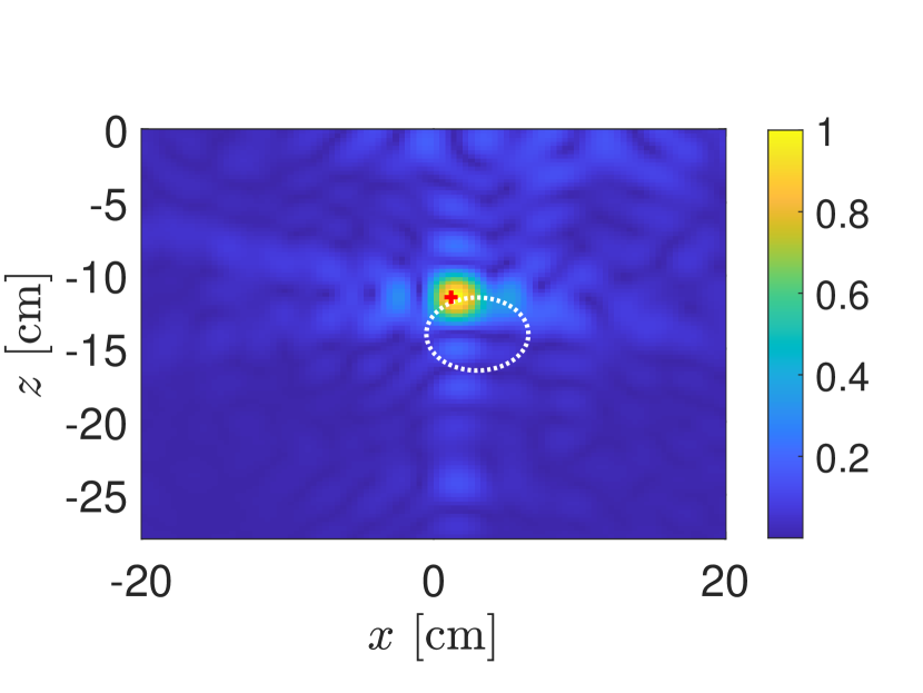
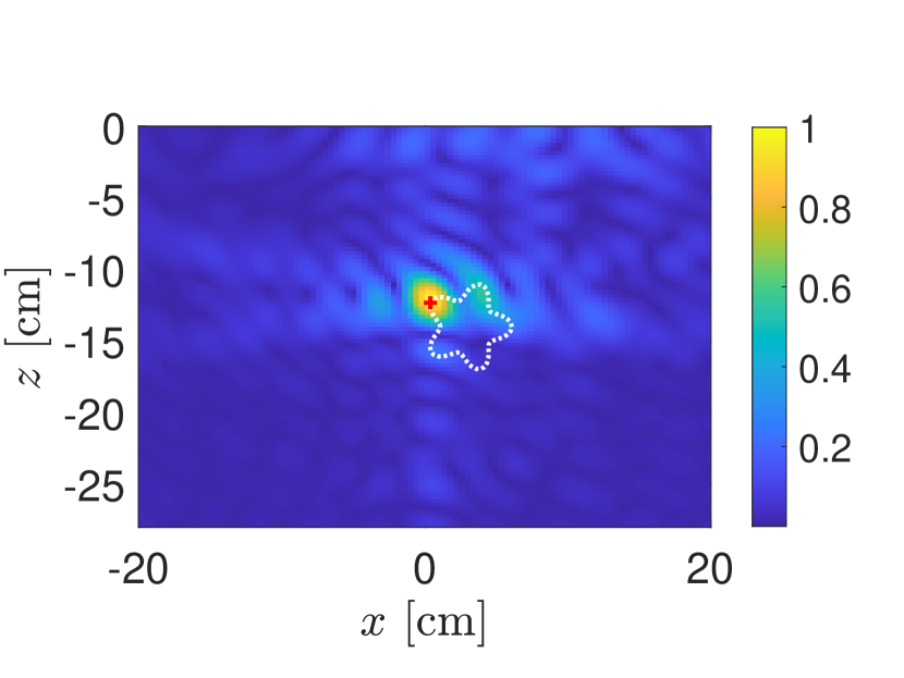
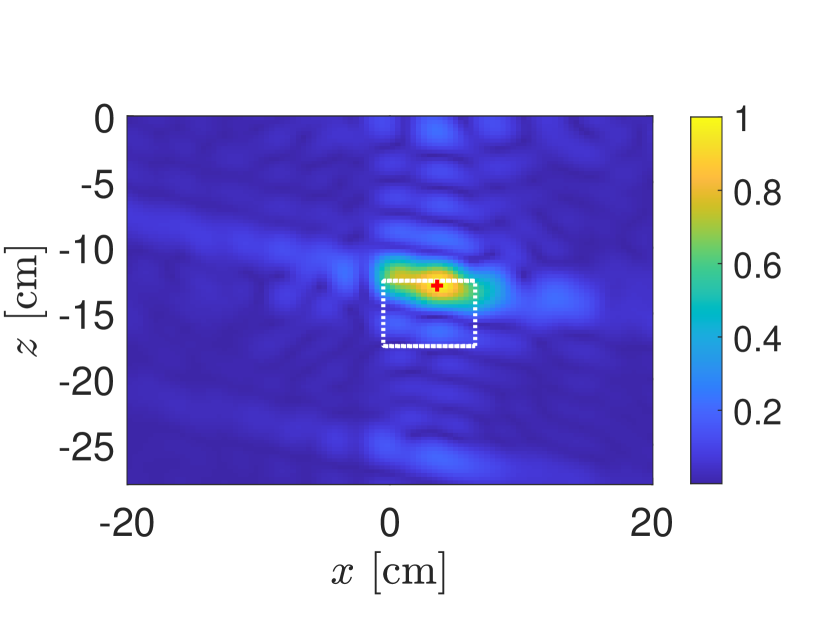
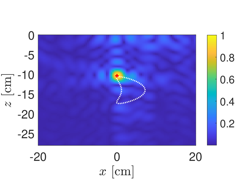
In Fig. 4 we consider the KM images for differently shaped targets: (a) a circle of radius cm centered at cm, (b) an ellipse with major axis cm and minor axis cm centered at cm, (c) a star whose boundary is given by cm for , and (d) a rectangle with width cm and height cm centered at cm. All of the targets have relative dielectric constant . All of these images have used PCA processed data and these KM images show plots of the absolute value of (19) normalized by its maximum value.
The maximum value of each of the KM images in Fig. 4(a)–(d) are plotted as a red “+” symbol. All of these results indicate that the KM image concentrates on a single point near the boundary of the target facing the synthetic aperture. There are some differences of the spread of the KM image about that point most notably for the rectangle. Nonetheless, these KM images do no provide too much spatial information other than this point. This behavior of KM images is due to the limitations in measurements. Specifically, SAR measurements (17) only subtend a relatively small portion of all scattering angles. Moreover, monostatic SAR measurements are restricted to just the backscattering or retroreflected direction. These space/angle limitations correspond to a severely limited aperture imaging problem. We cannot expect to recover very much spatial information about the target. The images shown in Fig. 4 suggest that one cannot obtain much more than a single point associated with a target. This point can be used to identify a target and locate it, but not much else.
V Measurement model
The results shown in the examples above suggest that there may be a simplified model for measurements. In what follows, we identify, test, and validate simplifying assumptions leading to a simplified model. We then propose how to use this simplified model for quantitative imaging of subsurface targets.
V-A First-order target-interface interactions
The first simplifying assumption we make is to consider only first-order interactions between the target and the air-soil interface. Even when there is multiple scattering in the direct scattering problem, methods for the inverse scattering problem based only on first-order interactions are effective. It is understood that these first-order interaction approximations carry sufficient phase information regarding boundaries where discontinuities in wave fields occur.
Assuming only first-order interactions between the target and the air-soil interface, we can consider the following procedure to approximate the solution of the direct scattering problem.
-
1.
For a source located above the air-soil interface, compute reflection and transmission by the rough air-soil interface with no target below it.
-
2.
Use the field transmitted across the air-soil interface to determine the field incident on the target.
-
3.
Solve the scattering problem by the target using that incident field.
-
4.
Compute the field scattered by the target that is transmitted back across the air-soil interface from soil into air and evaluate that result at the receiver.
Using block system (15) for the MFS implementation we have used here, this procedure corresponds to first solving
| (21) |
then solving
| (22) |
and finally solving
| (23) |
With these results, we approximate measurements through evaluation of (4) using .
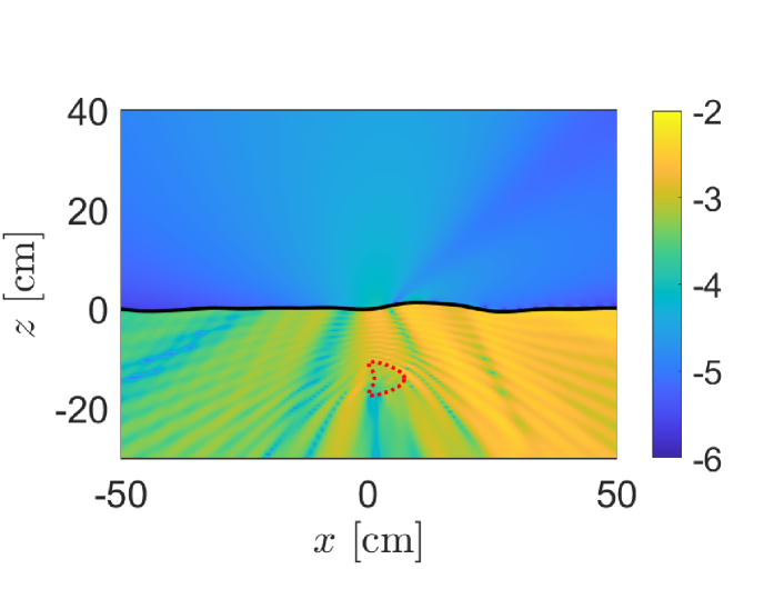
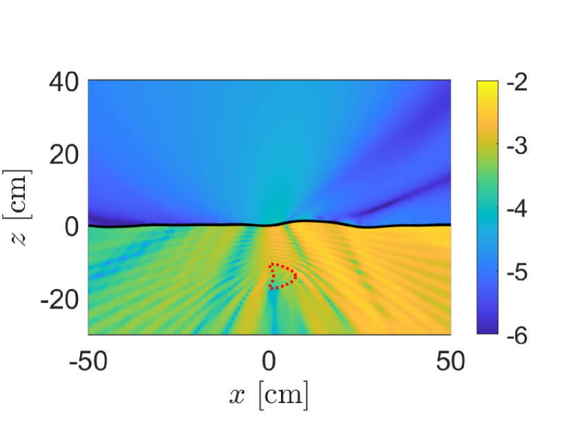
In Fig. 5 we show the absolute difference (-scale) between the MFS solution of the full boundary value problem described in Section III and the first-order target-interface interaction approximation described here. For these results, we have used one realization of a Gaussian-correlated random rough surface with RMS height cm and correlation length cm. The relative dielectric constant for soil is and for the target is . We used a point source at location cm at frequency GHz.
This result is characteristic of this first-order target-interface interaction approximation. The absolute difference is nearly three orders of magnitude smaller above the air-soil interface than below it. This non-uniformity is to be expected since the multiple interactions between the target and interface that are neglected in this approximation are most pronounced below the air-soil interface. However, from the point of view of modeling measurements taken above the air-soil interface, this result suggest that this approximation is accurate and useful simplifying the model of SAR measurements.

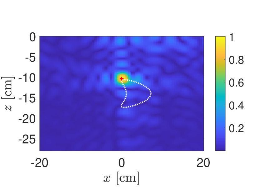
In Fig. 6 we show comparisons of the KM images produced using measurements computed (a) from the full direct scattering problem and (b) from the first-order target-interface interaction approximation. The air-soil interface is the same realization of a Gaussian-correlated random rough surface with RMS height cm and correlation length cm for both data sets. The relative dielectric constant in soil is and in the the target is . Additive measurement noise has been added so that SNR dB. Both of these images are produced using from their respective data matrices. These results are nearly indistinguishable from one another indicating that the first-order approximation is valid for modeling measurements. The location where the maximum of the KM image is attained for the first-order approximation is exactly the same as for for the full direct scattering problem data.
V-B Shower curtain effect
The shower curtain effect is a phenomenon related to imaging through a scattering medium [14, 15]. To explain it consider a source and a detector separated by a fixed distance with some multiple scattering region of finite extent (i.e. the shower curtain) somewhere in between. The location of the shower curtain relative to the source affects the image quality. Blurring is stronger when the shower curtain is closer to the receiver than the source. When the shower curtain is closer to the source, blurring is reduced in comparison. Scattering by the shower curtain causes blurring through introducing angular diversity. When the receiver is close to the shower curtain, it measures a substantial fraction of large-angle scattered fields which, in turn, introduces a mixture of phases that cause blurring. In contrast, when the receiver is far from the shower curtain, it does not measure those large-angle scattered fields thereby reducing blur.
When we use the first-order target-interface approximation described above, scattering by the target is a secondary source below the rough air-soil interface which acts as the shower curtain. Since a buried landmine is typically situated at distances on the order of the wavelength below the air-soil interface, its distance to it is shorter than the distance from the UAV to it. Considering the shower curtain effect, we assume that the roughness of the air-soil interface can be neglected when computing scattering by the target. For that case, we solve (21) and (22) as before, but replace (23) with
| (24) |
where the entries of the blocks , , , and are computed as (11) but for a flat air-soil interface in which for . We call this approximation the first-order/flat interface approximation.
In Fig. 7 we show results using this first-order/flat interface approximation for the same problem as in Fig. 5. The absolute difference (-scale) between the MFS solution for the full boundary value problem and this first-order/flat interface approximation is shown in Fig. 7(a). In comparison with Fig. 5 we see that the error for this approximation in the region above the air-soil interface is not markedly different and suggests its validity for modeling measurements.
To test its validity for modeling measurements for imaging, we show in Fig. 7(b) the resulting KM image normalized by its maximum value using of the data simulated using this approximation. The rough air-soil interface is the same one used for the results shown in Fig. 6. Additionally, we have added measurement noise to the approximate measurements so that SNR dB just as with the results shown in Fig. 6. This image formed using the first-order/flat interface approximation to simulate measurements is nearly indistinguishable with those shown in Fig. 6. Moreover, the location where the KM image attains its maxiumum value is exactly the same as that in Fig. 6(a). In the context of faithfully reproducing KM imaging results, these results show that this first-order/flat interface approximation is sufficiently accurate.
V-C Point target
All of the KM images we have shown exhibit a concentration about a single location where the KM image attains maximum value. The image for the rectangular target shown in Fig. 4(d) is the most different in that the concentration of the image about that point seems to follow the flat boundary. As we discussed in Section IV, this GP-SAR problem is a severely limited aperture imaging problem so we do not expect to recover much spatial information about the subsurface target. In light of these severe limitations, we consider simplifying a model of measurements by restricting our attention to a point-like target.
We know from elementary scattering theory that the field scattered by a particle in the far-field is proportional to the free-space Green’s function modified by a scattering amplitude [14]. It is the scattering amplitude that contains information about the particle such as its size, shape, and material properties. Limitations in GP-SAR measurements result in a severely limited sample of the scattering amplitude, but the KM images suggest the underyling Green’s function is robustly obtained.
Suppose we approximate the target below a rough air-soil interface by a point target located at below a flat air-soil interface. To consider a point target model within the MFS implementation we have used here, we solve (21) as before, but instead of solving (22) and (23), we instead solve
| (25) |
with
| (26) |
denoting the field exciting the point target. The components of the -vectors and are given by
| (27a) | ||||
| (27b) | ||||
for , respectively. We call the scalar parameter the reflectivity which gives the scattering strength of the point target.
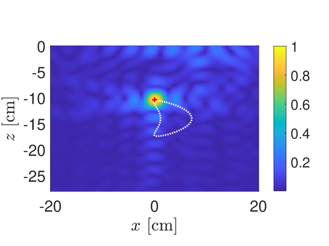
In Fig. 8 we show the KM image using the first-order/flat interface approximation with a point target located at cm. This target location corresponds to the location where the KM image attains its maximum value using the full direct scattering problem measurements. The reflectivity has been arbitrarily set to . Additive noise has been added to these approximate measurements so that SNR dB.
The KM image shown in Fig. 8 is nearly indistinguishable with all other images shown here. This result strongly indicates that this first-order/flat interface approximation with a point target model captures the spatial information contained in measurements based off of the full direct scattering problem. Alternatively, these results suggest that any additional sophistication in modeling measurements is lost when considering KM images of targets.
V-D Modeling GP-SAR measurements
Recall that entry of the data matrix gives the measurements at frequency at spatial location . We have discussed the following simplifying approximations above.
-
(i)
First-order target-interface interaction
-
(ii)
Flat interface for scattering by the target
-
(iii)
Point target model
The results above show that within the context of KM imaging these approximations are valid in that they faithfully capture the qualitative features of KM images using data simulated from solutions of the full boundary value problem. These approximations lead to the following model for GP-SAR measurements of a subsurface target:
| (28) |
with the matrix containing ground bounce signals by the rough air-soil interface, and the matrix containing signals scattered by a point target at location with reflectivity situated below a flat air-soil interface.
Within the context of this model, we can interpret the PCA and KM imaging method we have discussed above as follows. After computing the SVD of the measurements: , we compute
| (29) |
with
| (30) |
denoting the error in removing the ground bounce signal using the contributions made by the first singular values. When is small, it acts effectively as additive noise to . The evaluation of given in (19) with illuminations (20) is designed to “unwind” the phase accumulated through propagation of the scattered field by a point-like target below a flat air-soil interface at the search location . Consequently, when the search point is in a neighborhood of the point target position, the phases of the data and illuminations match and lead to the absolute value developing a peak.
By systematically testing and validating each of the simplifying assumptions above, we have established the validity of model (28). A key point to this model is the recognition of the limitations in GP-SAR measurements and understanding how those limitations affect the overall information content in those measurements. This model provides valuable insight into how the PCA and KM imaging method we have used here works.
V-E Extensions
Although our study uses only simulations of the direct scattering problem for scalar waves in two dimensions, the principles behind these basic assumptions extend naturally to more complicated three-dimensional scattering problems. For that case, the entries of matrices and correspond to the respective field values for the three-dimensional problem. Moreover, measurement model (28) can be modified to incorporate more sophistication when that is necessary. For example, we can include additional matrices for multiple subsurface targets. If the point target model is not valid for a related, but different problem, one can replace the matrix with a more sophisticated scattering model.
We have recently proposed a dispersive point target model where the reflectivity varies with frequency [16]. That target model is easily incorporated in (28) as
| (31) |
where corresponds to the reflectivity at frequency . From this dispersive point target model, we easily extend it further to include anisotropy in the reflectivity using
| (32) |
with denoting the Hadamard (element-wise) matrix product. The entries of the matrix are the reflectivities which now vary in frequency and space. These two extensions open opportunities for quantitative imaging methods that seek to determine reflectivities rather than seeking to determine spatial information about targets. Given the inherent space/angle limitations in GP-SAR measurements, these quantitative imaging problems may be more practically useful than seeking to find more spatial information about targets.
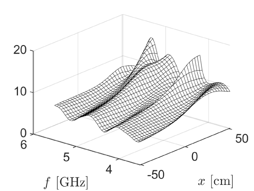
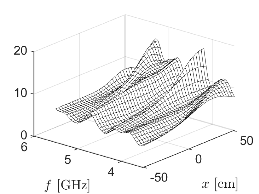
To investigate the validity of (32), we consider and that we used to evaluate the point target assumption in Fig. 8. We then consider the measurements used for Fig. 7 that used the first-order target-interface approximation and scattering by the kite-shaped target below a flat air-soil interface. To determine the reflectivity matrix , we subtract from those measurements and then divide that result element-wise by the entries of . A plot of the absolute values of this result are shown in Fig. 9(a), which we have labelled as “model.” We do the same computation using the measurements from the full direct scattering problem and those results are shown in Fig. 9(b), which we have labelled as “data.” These results show that the measurements computed from full direct scattering problem can be modeled accurately using (32) which includes the reflectivity matrix .
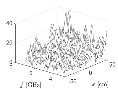
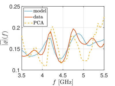
The results shown in Fig. 9 make explicit use of which tacitly implies that the rough air-soil interface is known. We now assume it is not known and apply PCA as we have done above by truncating the contributions made by the first two singular values to obtain . For that case, we estimate the reflectivity matrix by dividing element-wise by the entries of . A plot of the absolute values of this result are shown in the right plot of Fig. 10. This result shows that this estimate has large, spurious oscillations due to the error introduced in (30). Although only acts as additive measurement noise for imaging using KM, its effect on estimating here is much stronger. In light of these strong oscillatory errors, we consider the spatial average of absolute values:
| (33) |
Then we normalize this spatial average by its -norm and denote it by . A plot of for the results shown in Fig. 9 and this PCA result are shown in the right plot of Fig. 10. Even though these normalized frequency spectra do not quantitatively agree with one another, they share several characteristic features, especially within the sub-band between GHz and GHz.
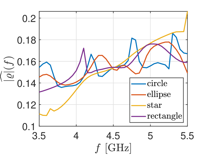
In Fig. 4 we showed that the imaging method we use here does not produce images that show clear differences for markedly different target shapes. In Fig. 11 we show for each of these targets. These results show that these frequency spectra are markedly different for the different targets. We have recently studied how these normalized frequency spectra can be used to classify subsurface targets [17]. From these results we see that there is characterizing information contained in GP-SAR measurements. By considering (32), we are able to propose novel quantitative methods that enable target classification.
VI Conclusions
We have studied GP-SAR imaging of subsurface targets below a rough air-soil interface. The imaging method we have used first uses principal component analysis to approximately remove ground bounce signals. Then it uses Kirchhoff migration on this processed data to identify and locate targets. By systematically studying and validating simplifying assumptions for modeling measurements, we have proposed the simplified model (28). This model is the sum of ground bounce signals by the rough air-soil interface and scattered signals by a point target below a flat air-soil interface. This simple model provides valuable insight into how the imaging method we have used here works.
The first assumption we discussed uses only first-order interactions between the target and the air-soil interface. Using first-order interactions is often done in inverse scattering problems for waves in a multiple scattering medium. The key to this approximation is that first-order interactions still retain crucially important phase information from scattering by the target. This phase information corresponds to discontinuities at boundaries and interfaces enabling the identification and location of targets.
The assumption that measurements of the signals scattered by the subsurface target can be modeled using a flat air-soil interface is a consequence of the so-called shower curtain effect. Because measurements are typically taken farther away from the air-soil interface than the distance between the target and interface, the effect of surface roughness on measurements is relatively small. This assumption is important because it relieves an imaging method from having to know the roughness of the air-soil interface.
The most extreme assumption used in this model is the point target model. The point target assumption is valid because of the inherent limitations in synthetic aperture measurements. Because this imaging problem is a severely limited aperture imaging problem, we do not expect to recover a lot of spatial information about the target. We have shown for the imaging method we have used here that we can recover only a representative point for the target. Consequently, a more sophisticated target model is not necessary.
Beyond the specific details of measurement model (28), it gives a theoretical framework for studying subsurface imaging problems. Moreover, the extended model (32) opens up new opportunities for quantitative imaging methods that may enable target classification. For these reasons, we believe that measurement model (28) is useful for studying GP-SAR imaging of subsurface targets.
References
- [1] G. L. Bier, “The economic impact of landmines on developing countries,” International Journal of Social Economics, vol. 30, no. 5, pp. 651–662, 2024/04/27 2003.
- [2] J. MacDonald, J. Lockwood, J. McFee, T. Altshuler, T. Broach, L. Carin, R. Harmon, C. Rappaport, W. Scott, and R. Weaver, Alternatives for landmine detection. Arlington, VA: Rand Coorporation, 2003.
- [3] M. García Fernández, Y. Álvarez López, A. Arboleya Arboleya, B. González Valdés, Y. Rodríguez Vaqueiro, F. Las-Heras Andrés, and A. Pino García, “Synthetic aperture radar imaging system for landmine detection using a ground penetrating radar on board a unmanned aerial vehicle,” IEEE Access, vol. 6, pp. 45 100–45 112, 2018.
- [4] M. Garcia-Fernandez, A. Morgenthaler, Y. Alvarez-Lopez, F. Las Heras, and C. Rappaport, “Bistatic landmine and IED detection combining vehicle and drone mounted GPR sensors,” Remote Sensing, vol. 11, no. 19, p. 2299, 2019.
- [5] J. Baur, “Ukraine is riddled with landmines. Drones and AI can help,” IEEE Spectrum, vol. 61, no. 5, May 2024.
- [6] R. Mathon and R. L. Johnston, “The approximate solution of elliptic boundary-value problems by fundamental solutions,” SIAM J. Numer. Anal., vol. 14, no. 4, pp. 638–650, 1977.
- [7] T. Wriedt, A. Doicu, and Y. Eremin, Acoustic and Electromagnetic Scattering Analysis Using Discrete Sources. Academic Press, 2000.
- [8] A. H. Cheng and Y. Hong, “An overview of the method of fundamental solutions—solvability, uniqueness, convergence, and stability,” Engineering Analysis with Boundary Elements, vol. 120, pp. 118–152, 2020.
- [9] A. D. Kim and C. Tsogka, “Intensity-only inverse scattering with MUSIC,” J. Opt. Soc. Am. A, vol. 36, no. 11, pp. 1829–1837, 2019.
- [10] A. H. Barnett and T. Betcke, “Stability and convergence of the method of fundamental solutions for helmholtz problems on analytic domains,” J. Comput. Phys., vol. 227, no. 14, pp. 7003–7026, 2008.
- [11] L. Tsang, J. A. Kong, K.-H. Ding, and C. O. Ao, Scattering of electromagnetic waves: numerical simulations. John Wiley & Sons, 2004.
- [12] R. Potthast, “A survey on sampling and probe methods for inverse problems,” Inverse Problems, vol. 22, no. 2, p. R1, 2006.
- [13] D. J. Daniels, “A review of GPR for landmine detection,” Sensing and Imaging, vol. 7, no. 3, pp. 90–123, 2006.
- [14] A. Ishimaru, Wave Propagation and Scattering in Random Media. New York: IEEE, 1997.
- [15] J. Garnier and K. Sølna, “Shower curtain effect and source imaging,” Inverse Probl. Imaging, vol. 18, no. 4, pp. 993–1023, 2024.
- [16] A. D. Kim and C. Tsogka, “Synthetic aperture imaging of dispersive targets,” IEEE Transact. Comput. Imaging, vol. 9, pp. 954–962, 2023.
- [17] ——, “Spectral classification of targets below a random rough air-soil interface,” IEEE Geosci. Remote Sensing Lett., to appear.