Modeling dynamic volatility under uncertain environment with fuzziness and randomness

Intra-day-sampled log returns of financial time series have many common stylized features (such as heavy tails, volatility clustering, long-term correlation, etc), which have been successfully captured by the stochastic volatility model with the Lévy process in the previous literatures. BN-S model is a popular stochastic volatility model with non-Gaussian (OU) process (Lévy process), which is often used to analyze the random behavior characteristics of asset price process in the research field of non-parametric methods of high-frequency time series. In the BN-S model, asset price dynamics are driven by Brownian motion, and price volatility is described by the Lévy process. We give a brief review of the original BN-S model.

In a financial market, a risk-free asset with a constant rate of return r and a risk asset (stock) are traded at a fixed horizon time $T$. The BN-S model assumes that the risk asset price process $S=(S_{t})_{t\geq 0}$, defined in a filtered probability space $(\Omega,\mathcal{F},(\mathcal{F}_{t})_{0\leq t\leq T},\mathbb{P})$, is given by

$\mathbb{P}$ is considered to be log prices, which follow the Black and Scholes type dynamics, with stochastic volatility driven by a non-Gaussian OU process. The log-return $X_{t}$ is controlled by

where $\sigma_{t}$ is the volatility at time $t$. And the parameters $\mu,\beta,\rho$ are constants, $\rho\leq 0$. The variance process is given by

here $\lambda$ is constants, and $\lambda>0$. For the physical probability measure $\mathbb{P}$, in this model, stochastic process $W=(W_{t})$ is a standard Brownian motion. Observe that BN-S model is driven by an incremental Lévy process of positive mean recovery, and the stochastic process $Z=(Z_{\lambda t})$ is the subordinator (background driving Lévy process, BDLP), where the processes $W$ and $Z$ are independent, and $(\mathcal{F}_{t})$ is a conventional enhancement of the filtering produced by $(W,Z)$. Solving formula (2.3), $\sigma_{t}^{2}$ could be given explicitly by

Obviously, the volatility process $\sigma_{t}^{2}$ is constrained by the deterministic function $e^{-\lambda t}\sigma_{0}^{2}$, and is strictly positive on $[0,T]$.

Compared with the non-parametric models, the BN-S model is easy to implement mathematically (without assuming that the volatility process obeys a certain distribution, the parameter estimation process is simpler and the estimation efficiency is higher), and could grasp the main characteristics of the realized volatility in the actual market (peak and thick tail, etc.) and the leverage effect of the price itself when describing the asset price change. However, with the continuous research and the development of technique, BN-S model cannot fully adapt to the actual financial market. With the aim of improving the theoretical framework of the model, we consider the price influence conditions in the classical BN-S model, and improve model based on the following two perspectives.

Firstly, improve the description of uncertain market information in original model. As mentioned in the introduction, many literatures have proved that the uncertainty of financial market includes randomness and fuzziness, which have a certain correlation, but can’t replace each otherbian2021fuzzy ; anzilli2018pricing ; zmevskal2022soft . It is necessary to consider both randomness and fuzziness so as to comprehensively describe the evolution process of asset price. The classical model only considers the randomness of the price process and ignores the fuzziness. Therefore, in subsection 2.2, we propose a fuzzy random representation of the asset price process, replace the historical price with the corresponding fuzzy number, and treat the asset price process as a fuzzy random process, which are applied to a new generalized BN-S model.

Secondly, solve the problem that BN-S model lacks long-range dependence. Some studies have shown that the superposition of OU processes can effectively improve the long-range dependence of financial random volatility model barndorff2001superposition . Considering the asynchronous phenomenon of asset price jump and volatility jump caused by the delay of market information dissemination, some recent literatures constructed the BDLP of BN-S model through two mutually independent Lévy processes, and achieved the accurate jump capture of crude oil, stock index, option and other financial assets over a long period of time salmon2021fractional ; sengupta2021refinements . Motived by these facts, in subsection 2.3 we use the superposition of two independent fuzzy Lévy processes to creatively construct a new generalized BN-S model that could be used in uncertain environment with fuzziness and randomness, and analyze the advantages of the new model.

The change of asset price is usually a continuous process, while the empirical price we obtained is discrete and static. The observable price sampling data eliminates some effective information about price changes in the sampling interval, and can’t accurately describe the asset price process in the sampling interval. Although the application of high-frequency data solves the above difficulties to a certain extent (frequent sampling reduces the neglected effective information in the sampling interval), but there are still more problems. For example, high-frequency data often carry more invalid information, and serious market microstructure noise makes it difficult to guarantee the unbiasedness and consistency of the realized volatility estimate.

Fuzzy theory could be used to solve the above problem. The discrete asset prices we observed naturally have fuzzy attributes. For example, the price of a stock is $100 at a certain time. $100 only represents the static price at one point. In fact, the dynamic price at some point should be described as around $100. This fact is difficult to describe from the perspective of probability theory. The observed price dynamics could be described as an interval number with membership function from the perspective of fuzzy theory.

We consider implementing two steps of asset price fuzzy representation in the study of dynamic volatility estimation. In the construction of generalized BN-S model, fuzzy random variables could be used to replace the random variables in the original model, and the asset price process would be regarded as a fuzzy random process. At the same time, in the data preprocessing, the fuzzy price could be used to describe the uncertain market information, and the historical price would be replaced by the corresponding fuzzy number.

Now give a brief introduction to the properties and calculation rules of fuzzy numbers, triangular fuzzy numbers, fuzzy random variables in fuzzy theory used in the study of dynamic volatility in fuzzy random uncertain environment.

Suppose that there is a fuzzy set $\tilde{a}$ on domain $S$, where $x$ is any element on all real numbers set $\mathbb{R}$, $\mu_{\tilde{a}}(x)\in[0,1]$ is the membership function of $\tilde{a}$. Membership (confidence) $\alpha$ is usually expressed as $\tilde{a}_{\alpha}=\{x:\mu_{\alpha}\textgreater\alpha\}$. The $\alpha^{-}$ level set of $\tilde{a}$ is composed of all elements whose membership degree to $\tilde{a}$ is not less than $\alpha$. Fuzzy number $\tilde{a}_{\alpha}$ is defined as $\tilde{a}_{\alpha}=\mu_{a}(x)=[\tilde{a}_{\alpha}^{L},\tilde{a}_{\alpha}^{U}],\alpha\in[0,1]$, where $\tilde{a}_{\alpha}^{L}$ is used to describe the degree of support for $x\in a$, which is the lower bound of membership; and $\tilde{a}_{\alpha}^{U}$ represents the upper bound of membership, describing the degree of opposition to $x\in a$.

In this paper, fuzzy price is used to describe the set of all prices in the sampling interval instead of the real closing price at a certain point. Fuzzy price is the expectation of an interval number. The lower limit of the interval is the lowest price in the sampling period, and the upper limit of the interval is the highest price in the sampling period. Of course, the closing price is also critical. The membership function of fuzzy price interval represents the membership degree of closing price to all price sets.

One of the classical expressions of fuzzy numbers is triangular fuzzy numberal2021ishita . The membership function of triangular fuzzy number was defined by

This function is a continuous convex function, which is composed of linear non decreasing function and linear non increasing function. The real number $\tilde{a}_{\alpha}^{m}$ is called the core value of triangular fuzzy number $\tilde{a}$. The real number $\tilde{a}_{\alpha}^{l}$ and $\tilde{a}_{\alpha}^{u}$ are respectively called the left and right spreads of $\tilde{a}$, represent the lower and upper limits of membership. And their difference shows the fuzzy degree of $\tilde{a}$.

The application of triangular fuzzy numbers is considered suitable for accurately describing the fuzzy properties of asset prices. We use the closing, the highest, and the lowest price as the core value, left and right spreads of the triangular fuzzy price. Compared with the price at sampling time point, which is concerned by previous stochastic volatility models, the triangular fuzzy price not only contains the price information of the sampling time point, but also describes the extent and distribution of dynamic price changes.

In fuzzy stochastic volatility models, fuzzy price calculations are inevitable. We list some basic arithmetic rules for triangular fuzzy numbers.

If $\tilde{a}_{\alpha}^{l}=\tilde{a}_{\alpha}^{m}=\tilde{a}_{\alpha}^{u}$, the fuzzy set $\tilde{a}$ degenerates into real number $\tilde{a}_{\alpha}^{m}$. In other words, the fuzzy price is equal to the historical closing price if the asset price did not fluctuate during the sampled period. The $\alpha^{-}$ level set of $\tilde{a}$ is $\tilde{a}_{\alpha}=[\tilde{a}_{\alpha}^{m}-(1-\alpha)\tilde{a}_{\alpha}^{l},\tilde{a}_{\alpha}^{m}+(1-\alpha)\tilde{a}_{\alpha}^{u}]$, where $\tilde{a}_{\alpha}^{L}=\tilde{a}_{\alpha}^{m}-(1-\alpha)\tilde{a}_{\alpha}^{l}$ and $\tilde{a}_{\alpha}^{U}=\tilde{a}_{\alpha}^{m}+(1-\alpha)\tilde{a}_{\alpha}^{u}$. If $\tilde{a}_{\alpha}^{L}$ and $\tilde{a}_{\alpha}^{U}$ are integrable, the expectation of $\tilde{a}$ is given by $E(\tilde{a}_{\alpha})=\frac{(1-\eta)\tilde{a}_{\alpha}^{l}+\tilde{a}_{\alpha}^{m}+\eta\tilde{a}_{\alpha}^{u}}{2},\eta\in[0,1]$, where the value of $\eta$ is related to the attention of fuzzy boundary. In the calculation of fuzzy price expectations, the value of $\eta$ is influenced by the risk attitude held by market participants. When investors are risk averse or pessimistic about holdings of the underlying asset, they pay more attention to the bottom of the price change. In this case, the lower limit of fuzzy price is the most important. The value of $\eta$ ranges from $0$ to $0.5$ and tends to $0$ with increasing pessimism or risk aversion. On the contrary, the upper limit of fuzzy price is more critical when decision makers are optimistic about the underlying assets or prefer risk. In this case, the value of $\eta$ is between $0.5$ and $1$, and tends to $1$ with the increase of optimism or risk preference. When the decision-maker takes a neutral attitude towards the risk of the underlying asset, $\eta=0.5$. In addition to the investor risk attitudes we discussed, there are other factors that affect the value of $\eta$, such as market trend, investment target, etc. In a rising bull market, the upper bound of the fuzzy price is more important than the lower bound, and the value of $\eta$ is generally between $0.5$ and $1$. In contrast, the value of $\eta$ in a bear market is usually less than $0.5$. Generally, the lower bound of put option price volatility is more concerned than the upper bound, so the value of $\eta$ tends to $0$ as the drop increases. While the value of $\eta$ describing the price dynamics of call options is always bigger than that of put options, and is generally between $0.5$ and $1$.

Note that the result of multiplication and division between real number $\gamma\not=0$ and triangular fuzzy number is still triangular fuzzy number, and the sum and difference of two triangular fuzzy numbers $\tilde{a}$ and $\tilde{b}$ are also triangular fuzzy numbers. For any membership $\alpha\in[0,1]$,

Under uncertain environment with fuzziness and randomness, the stochastic process in BN-S model could be replaced by fuzzy random process. A stochastic process is a set of random variables that depend on time. Correspondingly, fuzzy random process would be considered as a set of time-dependent fuzzy random variables.

Random variables with fuzzy forms are usually called fuzzy random variables, which have both randomness and fuzziness. Let $(\Omega,\mathcal{F},\mathcal{P})$ be a probability space with filtration satisfying standard assumptions, $\mathcal{B}$ is the Borel $\sigma^{-}$ field of all real numbers set $\mathbb{R}$, for every $\alpha\in[0,1]$ satisfying $\{(w,x)\in\Omega\times\mathbb{R}\mid\tilde{X}(w)(x)\geq\alpha\}\in\mathcal{F}\times\mathcal{B}$,the fuzzy-number-valued map $\tilde{X}:\Omega\longrightarrow\mathscr{F}$ is called a fuzzy random variablekwakernaak1978fuzzy . The $\alpha^{-}$ cut set of fuzzy random variable $\tilde{X}$ is a closed interval of the form $\tilde{X}=[\tilde{X}_{\alpha}^{L},\tilde{X}_{\alpha}^{U}]$, where $\tilde{X}_{\alpha}^{L}$ and $\tilde{X}_{\alpha}^{U}$ are general random variables. If $\tilde{X}_{\alpha}^{L}$ and $\tilde{X}_{\alpha}^{U}$ are integrable, $\forall\alpha\in[0,1]$, the expectation $E(\tilde{X})$ of $\tilde{X}$ could be written out as

where $l_{A}(x)$ is indicator function (if $x\in A,l_{A}(x)=1$, otherwise $l_{A}(x)=0$). The variance of $\tilde{X}$ is defined as

For two fuzzy random variables $\tilde{X}$ and $\tilde{Y}$, the variance of their sum is

and their covariance is

Their correlation coefficient is

with both $D\tilde{X}$ and $D\tilde{Y}$ are not $0$.

Applying the above fuzzy theory to the stochastic volatility model of risk asset price process, a fuzzy BN-S model was got. In this model, fuzzy stochastic price $\tilde{S}_{t}$ ,fuzzy log-return $\tilde{X}_{t}$ and fuzzy variance $\tilde{\sigma}_{t}^{2}$ of the stock or commodity are given by

where the parameters $\mu,\beta,\rho,\lambda$ are constants, and $\rho\leq 0,\lambda>0$. The process $W_{t}$ is a standard Brownian motion and $\tilde{Z}_{\lambda t}$ is a subordinator(background driving fuzzy Lévy process, BDFLP). And $\tilde{\sigma}^{2}=(\tilde{\sigma}_{t}^{2})$ is strictly positive.

Compared with the original model, fuzzy BN-S model has more advantages. Because the fuzzy random process carries more effective market information, the fuzzy model could describe the dynamic changes of price time series more accurately. In application, fuzzy price is applicable to all decision makers with different risk attitudes in the market. The change of risk attitude coefficient $\eta$ makes the model more flexible. The results of volatility estimation using fuzzy BN-S model have fuzzy attributes. Calculating the expectation value of fuzzy interval number is helpful to improve the accuracy of prediction results.

In this subsection, a new generalized BN-S model suitable for uncertain environment is introduced. Based on the fuzzy BN-S model, given by (5)(6)(7) shown in the previous subsection, the improved new model uses the superposition of two independent fuzzy random processes to fit the dynamic fluctuations of price and volatility.

Refer to a refined BN-S model shoshi2021hedging , assuming $\tilde{Z}_{\lambda t}$ and $\tilde{Z}_{\lambda t}^{*}$ to be two independent fuzzy Lévy subordinators with same (finite) variance. Like the fuzzy random process $\tilde{Z}_{\lambda t}$ independent of $W$ in (6), the new fuzzy Lévy subordination $\overline{Z}_{\lambda t}$ is defined as

where fuzzy random process $\tilde{Z}$ (including $\tilde{Z}_{\lambda t}$ and $\tilde{Z}_{\lambda t}^{*}$) and $\overline{Z}=(\overline{Z}_{\lambda t})$ are positively correlated Lévy subordinators.

Refer to dynamics of fuzzy stochastic price process of risky assets $\tilde{S}_{t}$ given by (5) and (6), and the new fuzzy Lévy subordination $\overline{Z}_{\lambda t}$ given by (8), fuzzy variance process $\tilde{\sigma}_{t}^{2}$ in (7) could be rewritten as

where $E(\tilde{\sigma}_{0})\not=0$. It is also a subordinate independent of $W$, and it is similar to $\tilde{Z}$ in (3) and $\overline{Z}$ in (7). $Z,\tilde{Z}$ and $\overline{Z}$ are positively correlated Lévy subordinators.

Given the constant influence of various information in the market, the price and volatility of risky assets may be affected to some extent and result in a series of changes. But these changes often do not happen at the same time. Because of the lag of market response, the jump of volatility and stock price are not always synchronized. As proposed insengupta2021refinements , considering (8) on the basis of (6), a new fuzzy log return $\tilde{X}_{t}$ with a convex combination of two independent subordinates $\tilde{Z}_{\lambda t}$ and $\tilde{Z}_{\lambda t}^{(b)}$ will be given by

where $\tilde{Z}_{\lambda t}$ and $\tilde{Z}_{\lambda t}^{(b)}$ are fuzzy random processes related to time parameter t and scale parameter $\lambda$. Jump measure $\tilde{Z}_{\lambda t}^{(b)}$ has greater Lévy intensity than jump measure $\tilde{Z}_{\lambda t}$. $\theta$ is a deterministic parameter,and $\theta\in[0,1]$. Specifically, for $\theta=1$, the original fuzzy stochastic process $\tilde{Z}_{\lambda t}$ will be replaced by $\tilde{Z}_{\lambda t}^{(b)}$. More intensive fuzzy stochastic process $\tilde{Z}_{\lambda t}^{(b)}$ means the big jumps. If there is no big jump, the value of $\theta$ is $0$. $\theta$ would be regarded as the deterministic component for completely stochastic dynamic price processes. And the value of $\theta$ in different periods could be estimated from empirical data. $(1-\theta)d\tilde{Z}_{\lambda t}+\theta d\tilde{Z}_{\lambda t}^{(b)}$ gives a flexible jump measure and accurately describes the dynamic characteristics of asset price fluctuations. In this case (9) will be given by

where, as $\theta$ in (10), $\theta^{{}^{\prime}}\in[0,1]$ is also deterministic. According to the operation rules of fuzzy random variables, $(1-\theta)d\tilde{Z}_{\lambda t}+\theta d\tilde{Z}_{\lambda t}^{(b)}$ is also a fuzzy Lévy subordination that is positively correlated with both $\tilde{Z}_{\lambda t}$ and $\tilde{Z}_{\lambda t}^{(b)}$. In this paper, we assume $\theta=\theta^{{}^{\prime}}$ for simplicity.

The expressions, given by (5), (10) and (11), of conditional distribution characteristic function of logarithmic price returns process in a new generalized BN-S model is derived. The parameter $\theta$ in (10) and (11), a deterministic component in a completely random price process, could be captured and predicted from historical data through machine learning and deep learning.

There is evidence that the dynamic process given by the new model contains long-term dependence. Suppose jump measures $J_{Z},\tilde{J}_{Z}$ and $\tilde{J}_{Z}^{(b)}$ are related to subordinators $Z_{\lambda t}$, $\tilde{Z}_{\lambda t}$ and $\tilde{Z}_{\lambda t}^{(b)}$ respectively, and $J(s)=\int_{0}^{s}\int_{\mathbb{R}+}J_{Z}(\lambda d\tau,dy)$, $\tilde{J}(s)=\int_{0}^{s}\int_{\mathbb{R}+}\tilde{J}_{Z}(\lambda d\tau,dy)$, $\tilde{J}^{(b)}(s)=\int_{0}^{s}\int_{\mathbb{R}+}\tilde{J}_{Z}^{(b)}(\lambda d\tau,dy)$; then for the log-return of BN-S model, fuzzy BN-S model, and generalized BN-S model mentioned above,

The instantaneous variance of log-return in (12) and (13) are $(\sigma_{t}^{2}+\rho^{2}\lambda Var(Z_{1}))dt$ and $(\tilde{\sigma}_{t}^{2}+\rho^{2}\lambda Var(\tilde{Z}_{1}^{(b)}))dt$ respectively. $Corr(X_{t},X_{s})$ will quickly become smaller as t increases for a fixed s. This decrease means that BN-S model and fuzzy BN-S model are affected by time t, which may lead to inaccurate result, that is, the models will fail seriously over a longer time. Note that in (14),the variance of log-returns $X_{t}$ is $\int_{0}^{v}\tilde{\sigma}_{\tau}^{2}d\tau+v\rho^{2}\lambda((1-\theta)^{2}Var(\tilde{Z}_{\lambda t})+\theta^{2}Var(\tilde{Z}_{\lambda t}^{(b)}))$, and the variance of log-returns $X_{s}$ is given by $\int_{0}^{v}\tilde{\sigma}_{\tau}^{2}d\tau+v\rho^{2}\lambda((1-\theta)^{2}Var(\tilde{Z}_{\lambda t})+\theta^{2}Var(\tilde{Z}_{\lambda t}^{(b)}))$. Unlike the results of the previous two models, the parameter $\theta$ is a dynamic value. For a fixed s in this model, the value of $\theta$ varies, $t$ always has an upper limit, and the model will never fail because $Corr(X_{t},X_{s})_{3}$ becomes “too small". This result proves that the new generalized BN-S model with fuzzy random processes incorporates long-range dependence. Our generalized BN-S model is believed to provide dynamic properties with distinct advantages when applied for modeling dynamic volatility under uncertain environment with fuzziness and randomness.

In conclusion, the new model has three advantages. Under uncertain environment, the fuzzy random variable in the new model is used to describe the fuzziness and randomness in the uncertainty of the financial market at the same time, to improve the utilization of information and the accuracy of results. In view of the jumps from price and volatility are not synchronized, a flexible and effective solution is proposed through less parameter changes. It has the advantage of long-range dependence, could be competent for volatility estimation in long time range, and expands the application range of BN-S volatility models. In the following, the new generalized BN-S model is tried to be used to analyze and predict the dynamic fluctuation of DJIA futures price in a fuzzy and random environment.

Considering the industry representativeness of DJIA futures listed in the Chicago Board of Trade (CBOT), this paper selects the high-frequency trading data of 1-year mini-sized DJIA futures (YM.CBT) as a sample to carry out dynamic volatility analysis. Its related stock index is DJIA, which is the most widely quoted stock index. The Futures contract months are March, June, September and December, which are listed and traded at all time of the year. Chicago Mercantile Exchange Globex electronic trading is from Sunday to Friday, from 6:00 p.m. to 5:00 p.m. of the next day (US Eastern time), and trading is suspended for 15 minutes from 4:15-4:30 p.m. (US Eastern time). We collected 66403 historical transaction data every 5 minutes in one year from two online data sources (Wind ¹¹1https://www.wind.com and Yahoo Finance²²2https://www.finance.yahoo.com). The time range of sample tracking is from 6:00 pm on September 30, 2020 to 5:00 pm on October 1, 2021. According to the sampling frequency of 5 minutes, 273 price data could be observed every day.

With the purpose of estimating the market volatility under uncertain environment with fuzziness and randomness, we implement the generalized BN-S model proposed in Section 2, and preprocess the historical data. Referring to the closing price at the sampling time and the historical price change range in the sampling interval, the triangular fuzzy price expectation, formed by the lowest price, closing price and highest price, would be used as the fuzzy price of the sampling interval.

Now we give the descriptive statistics of the sample of high-frequency mini-sized DJIA futures price after data preprocessing. Price is the key variable concerned in the study of dynamic fluctuation rule. But given the change of the closing price of mini-sized DJIA futures under the 5-minute sampling frequency is very small compared with the closing price itself. Direct observation of price can’t fully meet the accuracy requirements of high-frequency fluctuation research, and the small change of price may be ignored. With the view to pay full attention to the change dynamics of price, we consider the percentage change of price as one of the key variables. Table 1 provides descriptive statistics of price, fuzzy price and percentage change of them. When calculating the expectation of fuzzy price interval, $\eta$ represents different investment preferences. The expected value of price fuzzy set and the corresponding fuzzy price change percentage under different values of $\eta$ is showed in the table. Mean, median, minimum, maximum, skewness and kurtosis of eight variables about the mini-sized DJIA futures are reported.

The median of historical price change percentage is 0, indicating that the number of positive and negative fluctuations is basically balanced. In different market situations and investor preferences, the average number of fuzzy prices is distributed between 32521 and 32531.36, which shows that the fuzzy price of assets in the fuzzy random uncertain environment contains more market information than the historical price. For $\eta=0$, the value of fuzzy price is the smallest and the range of negative fluctuation is the largest, while the value of fuzzy price is the largest and the range of positive fluctuation is the largest for $\eta=1$. The skewness of observed price change percentage is greater than 0, and the kurtosis is far greater than 0, which indicate that there is a thick tail phenomenon on the right side and the characteristics of peak of the observation sample. This is consistent with the previous research conclusion of the peak thick tail in the return ratio sequence. The above data features are applicable to the generalized BN-S model with jump process mentioned in Section 2, Lévy process in the model could describe the dynamic changes of price time series.

In this subsection, we use visual analysis to understand the basic rule of mini-sized DJIA futures price time series fluctuation. We show the trend and distribution of fuzzy price, yield and realized volatility over time for $\eta=0.5$.

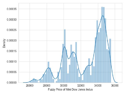
Figure 1 reports the distribution difference and change of fuzzy prices of mini-sized DJIA futures in each month of the year through the box chart. Obviously, the average price level in August 2021 is higher than that in other months. And the average level of the sample in October 2020 is the lowest. November 2020 has the largest price fluctuation. There were abnormal price changes in 7 months ( 10/2020, 12/2020, 1/2021, 2/2021, 5/2021, 6/2021, 7/2021 ), especially in September 2020 and October 2020.

As shown in Figure 2, the fuzzy price of mini-sized DJIA futures in one year is the most intensive in the range of $3400-3600$. Combined with figure 1, we could see that the prices after May $2021$ are mostly within this range, which shows that the overall fluctuation range of prices before May $2021$ is greater than that after May $2021$.

As mentioned in Subsection 3.2, the price change every 5 minutes is much smaller than the value of the price itself, so direct observation of the distribution of price change percentage would help us master a more precise information of sample dynamic change. Figure 3 is the histogram of fuzzy price change percentage of mini-sized DJIA futures. In the figure, the fuzzy price change statistics of mini-sized DJIA futures every 5 minutes can be positive or negative, mostly concentrated near $0$. The figure is not completely symmetrical and slightly skewed to the right, indicating that the number of prices experiencing rise and fall in the overall sample is similar, but the overall decline is less than the increase.

Now we observe the variation characteristics of realized volatility of mini-sized DJIA futures from the perspectives of numerical distribution and change trend. Figure 4 shows the realized volatility heatmap. By watching the black area and white area in the figure, the date with realized volatility change of more than $0.01\%$ could be identified. Obviously, November 2021 contains the largest number of volatile days. The realized volatility of each month has experienced frequent fluctuations. Figure 5 reports dynamic changes in realized volatility. The realized volatility of mini-sized DJIA futures has significant autocorrelation and volatility gathered. The sharp fluctuations are mainly concentrated near November 2021.

The analysis results in this section show that mini-sized DJIA futures always have volatility jumps of different amplitudes and frequencies in most periods of a year. For the sake of quantifying the jump characteristics in the fluctuation, we refer to the information of the data characteristics shown in the above chart and use the deep learning algorithms to estimate the parameters in the following section.

Based on the data analysis results in Section 3, in this section, we estimate the value of $\theta$ in the new model in Section 2. We create a classification problem as follows.

1) Index the available fuzzy price of mini-sized DJIA futures in chronological order.

2) Group the data according to the price fluctuation characteristics analyzed in Section 3 and create a new data structure. We try to take the percentage change of fuzzy price for $50$ consecutive minutes as a row subset and stack it layer by layer to form a new fuzzy price matrix.

3) Consider the fluctuation range of fuzzy price change percentage of mini-sized DJIA futures, determine the threshold $K$, and search for the “big jump". The time of each price data that is $K$ “points" lower than the fuzzy price of the previous 5 minutes will be identified. ( if $K=0.1\%$, record the time when the fuzzy price is $0.1\%$ lower than the previous one).

4) Create a target column $\theta$ for the new matrix. If there are at least two “big jumps" in the next $50$ minutes, the value of the target column $\theta$ of the row is $1$. Otherwise, the value of the corresponding $\theta$ is $0$.

5) Neural network algorithms will be used for sample data set learning and parameter $\theta$ estimation.

After completing the steps above, assign $\theta$ the results of classification report. The value of $\theta$ could be directly used in formulas (10) and (11) as a deterministic component in the stochastic volatility model.

In this subsection, we implement the steps in subsection 4.1 to calculate the results with reasonable accuracy $\theta$ to prove the operability of these steps. We run three common neural network algorithms ((a) standard neural network, (b) long short-term memory neural network and (c) LSTM network with batch normalizer (BN)) for classification calculation on python. The subset elements of each row in the new matrix are input parameters, and output parameter $\theta$ ($0$ or $1$) is the subset elements in the target column of the new matrix.

In a bid to report the applicability of the new model, the fluctuation rules of different time spans (intraday high-frequency data, daily data, weekly data and monthly data) should be taken into account. Referring to the sample characteristics in Section 3, We randomly select four classifiers from the preprocessed fuzzy price data for data training and data testing. The time periods of classifiers are

Aiming at the different risk preference, threshold $K$ mentioned in the classification problem could be adjusted to satiate investors. The threshold $K$ of different sizes also helps market regulators identify and deal with the future volatility risk. The value of $K$, specifically, is the condition for us to retrieve the target fluctuation. The shorter the observation interval, the smaller the range of observed-value changing in a fixed time interval. Therefore, high sampling frequency is often best matched with small value of threshold $K$, which would identify more jumps. We use different $K$ sizes for the fuzzy price classifications of mini-sized DJIA futures. Table 2 reports the number of jumps that could be identified when different sizes of threshold $K$ are set in the classifications.

Under different $K$ sizes, we use the three neural networks mentioned above to estimate the value of $\theta$. For the purpose of obtaining more accurate parameter estimation results, we set up four indicators to comprehensively evaluate the results of parameter prediction. “support" reports the number of jump samples in the test set, “precision" indicates the accuracy of the prediction results, “recall" refers to prediction efficiency, and “f1-score" shows the possibility of $\theta$ taking different values in the future. The classification reports are shown in Table 3-8.

The recognition results of the jumps number in historical price by use the three neural networks are always consistent. It shows that the three selected algorithms are all effective and accurate at the jump recognition stage.

Comparing table 3 and 4, we found that with the increasing of $K$, the numbers of response in $T1$ to $\theta=0$ increases significantly and that to $\theta=1$ gradually decreases. This result is in line with our expectation. In the same time interval, the more jumps could be captured with the lower threshold of jump recognition, and it is greater possibility of $\theta=1$, which means the stronger fuzzy random process $\tilde{Z}_{\lambda t}^{(b)}$ will be used to characterize the realized volatility dynamics.

The classification results in $T1$ show that it is more likely that the value of $\theta$ in the test set is $1$ when $KS=0.01$. And that’s the fact. When $KS=0.05$, all three algorithms suggest that $\theta=0$. These results show that the value of $\theta$ is affected by the size of threshold $K$. In other words, our new model could track and estimate jumps with different jump size and the jump intensity. It is flexible and suitable for investors and regulators with different purposes to grasp the change law of the market changes.

A similar conclusion is drawn in the comparison between table 5 and 6. For $KS=0.01$, the numbers of response to $\theta$ =0 is fewer than that to $KS=0.03$. The numbers of response to $\theta$ =1 is negatively correlated with the value of K. The results in tables 5 and 6 show that 1 is considered to be an appropriate value of $\theta$ for $KS\leq 0.03$ in $T2$. And the same results are reported in table 7 and 8. Where $\theta$ is suggested to be $0$ for $KS=0.05$ in T3 and $KS=0.1$ in $T4$. This means that, it is suitable for a weaker fuzzy stochastic process $\tilde{Z}_{\lambda t}$ used to characterize realized volatility dynamics.

Comparing the “support" in table 3 and 5, we find that the more jumps could be recognized with the increase of time span $T$. This rule would also be found by comparing the results in table 4 and 7.

In conclusion, both $K$ and $T$ can directly affect the number of recognized jumps, and then affect the value of $\theta$. The effect of value of $K$ on number of identifiable jumps was positive and significant, and the effect of $T$ length on number of identifiable jumps was negative and significant.

References

- \bibcommenthead
- (1) Gradojevic, N., Kukolj, D.: Unlocking the black box: Non-parametric option pricing before and during covid-19. Ann. Oper. Res., 1–24 (2022)
- (2) Zhang, Y., Ma, F., Liao, Y.: Forecasting global equity market volatilities. Int. J. Forecast. 36(4), 1454–1475 (2020)
- (3) Bian, L., Li, Z.: Fuzzy simulation of european option pricing using sub-fractional brownian motion. Chaos Solitons Fractals 153, 111442 (2021)
- (4) Shapiro, A.F.: Fuzzy random variables. Insur. Math. Econ. 44(2), 307–314 (2009)
- (5) Mbairadjim Moussa, A., Sadefo Kamdem, J.: A fuzzy multifactor asset pricing model. Ann. Oper. Res., 1–21 (2021)
- (6) Chen, J., Tang, G., Yao, J., Zhou, G.: Investor attention and stock returns. J. Finac. Quant. Anal. 57(2), 455–484 (2022)
- (7) Pawłowski, M., Nowak, P.: Stochastic approach to model spot price and value forward contracts on energy markets under uncertainty. J. Amb. Intel. Hum. Comp., 1–15 (2021)
- (8) Nowak, P., Pawłowski, M.: Pricing european options under uncertainty with application of lévy processes and the minimal lq equivalent martingale measure. J. Comput. Appl. Math. 345, 416–433 (2019)
- (9) Li, H., Ware, A., Di, L., Yuan, G., Swishchuk, A., Yuan, S.: The application of nonlinear fuzzy parameters pde method in pricing and hedging european options. Fuzzy Set Syst. 331, 14–25 (2018)
- (10) de Andrés-Sánchez, J.: Pricing european options with triangular fuzzy parameters: assessing alternative triangular approximations in the spanish stock option market. Int. J. Fuzzy Syst. 20(5), 1624–1643 (2018)
- (11) Saporito, Y.F., Yang, X., Zubelli, J.P.: The calibration of stochastic local-volatility models: An inverse problem perspective. Comput. Math. Appl. 77(12), 3054–3067 (2019)
- (12) Izzeldin, M., Tsionas, M.G., Michaelides, P.G.: Multivariate stochastic volatility with large and moderate shocks. J. R. Stat. Soc. A. Stat. 182(3), 887–917 (2019)
- (13) Yang, B.-Z., Yue, J., Wang, M.-H., Huang, N.-J.: Volatility swaps valuation under stochastic volatility with jumps and stochastic intensity. Appl. Math. Comput. 355, 73–84 (2019)
- (14) Yu, X.: On the convergence of two types of estimators of quadratic variation. Math. Meth. Appl. Sci. (2021)
- (15) Qin, L., Todorov, V.: Nonparametric implied lévy densities. Ann. Stat. 47(2), 1025–1060 (2019)
- (16) Barndorff-Nielsen, O.E., Shephard, N.: Econometric analysis of realized volatility and its use in estimating stochastic volatility models. J. R. Stat. Soc. B. 64(2), 253–280 (2002)
- (17) Fallahgoul, H., Hugonnier, J., Mancini, L.: Risk premia and lévy jumps: Theory and evidence. Swiss Financ. Inst. Res. Pap. (19-49) (2020)
- (18) Tan, X., Li, S., Wang, S.: Pricing european-style options in general lévy process with stochastic interest rate. Mathematics 8(5), 731 (2020)
- (19) Barndorff-Nielsen, O.E., Shephard, N.: Non-gaussian ornstein–uhlenbeck-based models and some of their uses in financial economics. J. R. Stat. Soc. B. 63(2), 167–241 (2001)
- (20) Chen, J., Wang, F., Chen, H.: Probability-conservative simulation for lévy financial model by a mixed finite element method. Comput. Math. Appl. 106, 92–105 (2022)
- (21) Gloter, A., Loukianova, D., Mai, H.: Jump filtering and efficient drift estimation for lévy-driven sdes. Ann. Statistics 46(4), 1445–1480 (2018)
- (22) James, L.F., Müller, G., Zhang, Z.: Stochastic volatility models based on ou-gamma time change: theory and estimation. J. Bus. Econ. Stat. 36(1), 75–87 (2018)
- (23) Posedel Šimović, P., Tafro, A.: Pricing the volatility risk premium with a discrete stochastic volatility model. Mathematics 9(17), 2038 (2021)
- (24) Corsaro, S., Kyriakou, I., Marazzina, D., Marino, Z.: A general framework for pricing asian options under stochastic volatility on parallel architectures. Eur. J. Oper. Res. 272(3), 1082–1095 (2019)
- (25) Chen, R., Zhou, H., Yu, L., Jin, C., Zhang, S.: An efficient method for pricing foreign currency options. J. Int. Financ. Mark. I. 74, 101295 (2021)
- (26) Bakhshmohammadlou, M., Farnoosh, R.: Hedging of options for jump-diffusion stochastic volatility models by malliavin calculus. Math. Sci. 15(4), 337–343 (2021)
- (27) Baule, R., Shkel, D.: Model risk and model choice in the case of barrier options and bonus certificates. J. Bank. Financ. 133, 106307 (2021)
- (28) Li, Y., Jiang, S., Li, X., Wang, S.: The role of news sentiment in oil futures returns and volatility forecasting: data-decomposition based deep learning approach. Energ. Econ. 95, 105140 (2021)
- (29) Aras, S.: On improving garch volatility forecasts for bitcoin via a meta-learning approach. Knowl. Based Syst. 230, 107393 (2021)
- (30) Samitas, A., Kampouris, E., Kenourgios, D.: Machine learning as an early warning system to predict financial crisis. Int. Rev. Financ. Anal. 71, 101507 (2020)
- (31) Lyócsa, Š., Molnár, P., Vỳrost, T.: Stock market volatility forecasting: Do we need high-frequency data? Int. J. Forecast. 37(3), 1092–1110 (2021)
- (32) Gu, S., Kelly, B., Xiu, D.: Empirical asset pricing via machine learning. Rev. Financ. Stud. 33(5), 2223–2273 (2020)
- (33) Company, R., Egorova, V.N., Jódar, L., Soleymani, F.: A stable local radial basis function method for option pricing problem under the bates model. Numer. Meth. Part. D. E. 35(3), 1035–1055 (2019)
- (34) Shoshi, H., SenGupta, I.: Hedging and machine learning driven crude oil data analysis using a refined barndorff-nielsen and shephard model. Int. J. Financ. Eng. 8(04), 2150015 (2021)
- (35) Awasthi, S., SenGupta, I.: First exit-time analysis for an approximate barndorff-nielsen and shephard model with stationary self-decomposable variance process. J. stoch. Analysis 2(1), 5 (2021)
- (36) You, C., Bo, L.: Option pricing based on a type of fuzzy process. J. Amb. Intel. Hum. Comp., 1–15 (2021)
- (37) Anzilli, L., Facchinetti, G., Pirotti, T.: Pricing of minimum guarantees in life insurance contracts with fuzzy volatility. Inf. Sci. 460, 578–593 (2018)
- (38) Zmeškal, Z., Dluhošová, D., Gurnỳ, P., Guo, H.: Soft bond game options valuation in discrete time using a fuzzy-stochastic approach. Int. J. Fuzzy Syst., 1–14 (2022)
- (39) Barndorff-Nielsen, O.E.: Superposition of ornstein-uhlenbeck type processes. Thero. Probab. Appl. 45(2), 175–194 (2001)
- (40) Salmon, N., SenGupta, I.: Fractional barndorff-nielsen and shephard model: applications in variance and volatility swaps, and hedging. Ann. Financ 17(4), 529–558 (2021)
- (41) SenGupta, I., Nganje, W., Hanson, E.: Refinements of barndorff-nielsen and shephard model: an analysis of crude oil price with machine learning. Ann. Data Sci. 8(1), 39–55 (2021)
- (42) Al-Qudaimi, A.: Ishita approach to construct an interval-valued triangular fuzzy regression model using a novel least-absolute based discrepancy. Eng. Appl. Artif. Intel. 102, 104272 (2021)
- (43) Kwakernaak, H.: Fuzzy random variables—i. definitions and theorems. Inform Sciences 15(1), 1–29 (1978)