Modeling Dynamic User Preference via Dictionary Learning for Sequential Recommendation
Abstract
Capturing the dynamics in user preference is crucial to better predict user future behaviors because user preferences often drift over time. Many existing recommendation algorithms – including both shallow and deep ones – often model such dynamics independently, i.e., user static and dynamic preferences are not modeled under the same latent space, which makes it difficult to fuse them for recommendation. This paper considers the problem of embedding a user’s sequential behavior into the latent space of user preferences, namely translating sequence to preference. To this end, we formulate the sequential recommendation task as a dictionary learning problem, which learns: 1) a shared dictionary matrix, each row of which represents a partial signal of user dynamic preferences shared across users; and 2) a posterior distribution estimator using a deep autoregressive model integrated with Gated Recurrent Unit (GRU), which can select related rows of the dictionary to represent a user’s dynamic preferences conditioned on his/her past behaviors. Qualitative studies on the Netflix dataset demonstrate that the proposed method can capture the user preference drifts over time and quantitative studies on multiple real-world datasets demonstrate that the proposed method can achieve higher accuracy compared with state-of-the-art factorization and neural sequential recommendation methods. The code is available at https://github.com/cchao0116/S2PNM-TKDE2021.
Index Terms:
Collaborative filtering, sequential recommendation, dynamic preference, dictionary learning1 Introduction
In recommender systems, user preferences often drift over time due to various reasons, e.g., changes in life [23], experience growth [40], etc. However, many existing collaborative filtering (CF) algorithms [41, 28] summarize a user’s historical records into a single latent vector, which may lose the dynamic preference drifts and lead to suboptimal recommendation accuracy [40, 23, 9]. To remedy this, many techniques have been adopted to model user dynamic preferences in collaborative filtering. For instance, Rendle et al. [47] and He et al. [16] both adopted Markov chains to model local patterns among items. Zheng et al. [68] used the neural autoregressive distribution estimator (NADE) to model the conditional probability of the next item given a user’s historical ratings. Recently, several works [21, 62, 2] used recurrent neural networks (RNN) to embed previously purchased products for current interest prediction. Due to the recent advances of deep learning, these RNN-based methods have achieved promising results in sequential recommendation. Our case study shows that RNN-based methods [62, 68] that consider sequential patterns exhibit better accuracy than state-of-the-art matrix approximation methods [28, 5, 34] without considering sequential information on the Netflix prize dataset.
However, existing RNN-based methods [62, 68, 65], which exhibit the advantage by capturing temporal or sequential user behaviors, may not be suitable for modeling and capturing the long-term impact of previously purchased items on the future one [9]. To remedy this, many works [60, 9, 25, 44, 64, 26, 67] proposed to use external memory networks (EMN) [61, 55] and attention mechanism [11, 57], where shorter path between any positions in the sequence makes the long-term impact easier to learn. Despite their effectiveness, the ordinal information of historical items is usually not explicitly considered in these works, which may lead to suboptimal performance because the sequential patterns contained in the sequence of user behaviors may be neglected. In addition, the sequential patterns may be conceptually different from user preferences, i.e., in different feature spaces, and thereby it may increase the complexity of learning the downstream estimators when user preferences are directly combined with the intermediate outputs of recurrent/memory/attention networks.
In this paper, we propose a dictionary learning-based approach to model both long-term static user preferences and short-term dynamic user preferences under the same latent space. More specifically, we learn a dictionary from scratch and each row of the dictionary can be regarded as a basis representing a partial signal of user dynamic preferences shared across all users. Then, the dynamic preference of each user can be modeled by a linear combination of all the rows in the dictionary. To achieve adaptive linear combination on different users / sequences, we propose a deep autoregressive model integrated with Gated Recurrent Unit (GRU) to learn features from user sequential behaviors, which can generate the weights for the linear combination to form the dynamic preference of each user. After obtaining the dynamic preference of each user, we use an additive mechanism to fuse the dynamic and static preferences for predicting the future interests of each user.
The main contributions of this work are summarized as follows:
-
1.
To the best of our knowledge, this is the first work that tackles the sequential recommendation problem via dictionary learning, which can model user static preferences and dynamic preferences under the same latent space to achieve simpler fusion, i.e., a simple additive mechanism can achieve decent performance.
-
2.
Sequence-to-preference neural machine (S2PNM) is proposed to translate the sequential behaviors of users into dynamic user preferences using a deep autoregressive model integrated with GRU.
-
3.
Empirical studies on multiple real-world datasets demonstrate that S2PNM can significantly outperform state-of-the-art factorization and neural sequential recommendation methods in recommendation accuracy.
2 Problem Formulation
This section first formulates the targeted problem and then presents a case study to show the challenge faced by existing CF methods without considering sequential information.
2.1 Matrix Factorization (MF)
Matrix factorization-based collaborative filtering algorithms have recently achieved superior performance in both rating prediction task [28, 5] and top-N recommendation task [20, 24]. Given a user-item rating matrix with users and items, we denote as the score rated by user on item at time . Then for each user, there always exists an item sequence ( will vary for different users). Traditional MF methods, e.g., regularized SVD (RSVD) [43], are popular due to simple implementation and superior accuracy compared to other kinds of methods. More formally, these methods generally minimize the sum-squared error between the rating matrix and its low-rank recovery with regularization as follows:
| (1) |
where are the latent factors of users and items respectively, and is an indicator function that equals to when is observed and equals to otherwise. is the Frobenius norm of .
2.2 Case Studies
Traditional MF methods [28, 5, 34] did not consider the sequential information, and thus may yield suboptimal performance in real scenarios in which user future interests are predicted on their historical behaviors. Here, we conduct a case study on the Netflix dataset to demonstrate that state-of-the-art MF methods indeed underperform in sequential-based data splitting protocol. More specifically, we adopt two different data splitting protocols on the Netflix dataset to study how the prediction accuracy varies: 1) random splitting, which is the most widely adopted protocol in classical collaborative filtering literature [28, 62]; and 2) sequential-based splitting, in which we split the dataset based on the chronological order to simulate real recommendation scenarios. To make a fair comparison, we keep the ratio of training and test sets as : for both data splitting protocols.
| Method | spit-by-random | spit-by-time |
| SVD++ | 0.80701 | 0.89267 |
| GLOMA | 0.80132 | 0.89326 |
| MRMA | 0.79940 | 0.89210 |
| RRN | 0.80443 | 0.89014 |
| NADE | 0.80243 | 0.88876 |
| S2PNM | 0.78481 | 0.87301 |
Table I summaries the recommendation accuracy in terms of RMSE on one baseline method (SVD++ [28]), two state-of-the-art MF methods (MRMA [34] and GLOMA [5]), two sequential recommendation methods (RRN [62] and NADE [68]), and meanwhile the proposed S2PNM method. As shown in the results, non-sequential methods (MRMA and GLOMA) achieved higher accuracy than sequential methods (RRN and NADE) on random splitting protocol but achieved lower accuracy on sequential-based splitting protocol. This confirms that capturing the correlations between user historical behavior and his/her future interests can help to achieve better recommendations in real scenarios. In addition, when comparing the numbers between the second column and the third column, we can see that the accuracies of GLOMA and MRMA are on par with the baseline method – SVD++ in the sequential-based splitting protocol whereas they significantly outperform SVD++ in the random splitting protocol. This indicates that conclusions made under the unrealistic random splitting protocol may not hold in the realistic setting, and therefore it is necessary to design and evaluate recommendation algorithms in the harder but more realistic sequential-based splitting protocol.
3 The Proposed Sequence-to-Preference Neural Machine

This section first presents the main building block of S2PNM – the Seq2Pref network in detail. Then, we discuss the choice of prediction function for recommendation scores. After that, we discuss the optimization problems for two recommendation tasks. At last, we discuss the parallel training of S2PNM.
3.1 Seq2Pref Network
3.1.1 Dictionary Learning
Dictionary learning aims to learn a set of vectors capable of succinct expression of the targeted events, i.e., a linear combination of the rows of the dictionary learned from the data can succinctly represent any piece of the input data [32, 39]. In this paper, we try to learn a dictionary that can construct sufficient representations of user dynamic preferences and meanwhile embed user dynamic preferences into the same latent space of user static preferences.
More formally, we propose to learn a feature dictionary such that the dynamic user preference of user at time — can be constructed by a linear combination of the rows in using the non-negative coefficients as follows:
| (2) |
Here, denotes the number of rows in the dictionary and denotes the number of hidden units to represent user preferences. The dictionary can be regarded as a collection of basis which is capable of modeling the changes of user preference vector according to his/her sequential behavior. Then, the combined preference vector of user at time can be modelled as follows:
| (3) |
where is the static user preference vector.
To learn the optimal dictionary for modeling user dynamic preferences, we can define a optimization objective as follows:
| (4) |
Here, is the rating vector of user and is the predicted rating vector at time . is the distance function between two vectors. Let and and be the F-norm. The above Eqn. 4 means that minimizing the discrepancy between the true ratings and predicted ratings is equivalent to minimizing the discrepancy between the residual error (true rating minus predicted rating from static user preferences) and the dynamic rating (computed from dynamic user preferences). Based on this idea, the above optimization objective can be reformulated as follows:
Therefore, modeling the dynamic user preferences can be formulated as a supervised dictionary learning problem, in which the dictionary D is randomly initialized and then optimized by gradient-based learning techniques. Note that the above Eqn. 4 only illustrates our main idea that the goal of the dictionary learning is to minimize the residual error of the predictions. More specifically, we use an end-to-end training for the whole model instead of training each part of the model individually. The final loss functions are presented in Section 3.3.
In the above dictionary learning problem, the posterior distribution should not be obtained via point estimations which are not feasible in test time. Therefore, different from standard dictionary learning problem [39], we propose to learn a state function , which allows us to accurately obtain from the user rating vector as follows:
| (5) |
denotes the complete rating history of user before time . Note that the learning of is challenging because (1) it should accurately capture the sequential dependencies within the rating sequence of each user and (2) it needs to embed the sequential dependencies into the same latent space as the downstream score estimator. To this end, we propose to use a RNN-based autoregressive model to capture the sequential dependencies, and then feed the learned information to the latent space via minimizing the loss .
3.1.2 Encoding Sequential Dependencies
This paper adopts GRU [10] with attention to learn user dynamic preferences. GRU can adaptively capture the sequential dependencies with different time scales which is more suitable to model the users with different rating time scales in recommendation problem. The neural attention mechanism permits learning an adaptive nonlinear weighting function, which allows the more (less) related dependency patterns to make more (less) contributions in the predictions.
Given the historical ratings of a user 111When training the model, we use the entire sequence without slicing, so that the length is variable for each user in a batch., we first put them into an embedding layer which outputs continuous vectors, then we feed these vectors to GRU to learn the sequential representations . Each hidden state after the -th historical item can be formally described as follows:
| (6) | |||
| (7) | |||
| (8) |
In Eqn. 6, GRU is used as a recurrent activation function which we refer to as a recurrency. Meanwhile, is the (-1)-th hidden state of GRU, and is a vector of the attention weights. Eqn. 7 describes a content-based multiplicative attention mechanism [11] which scores each element in separately and normalizes the scores using softmax as follows:
| (9) | |||
| (10) |
Here, we use a weighted mapping in stead of an identity mapping due to better empirical performance.
3.1.3 Decoding Dynamic User Preferences
After encoding the sequential dependencies in a rating sequence, we decode and embed these information into the same latent space of user static preference. More specifically, we learn a multi-layer perceptron (MLP) to approximate the posterior distribution in Eqn. 2, i.e., the output of the MLP is used as in Eqn. 2. Formally, we estimate the posterior distribution for the -th item rated by user as follows:
| (11) | |||
| (12) | |||
| (13) | |||
| (14) |
Here, the operator is the element-wise product and in Eqn. 11 can capture the second-order interactions between the learned sequential dependencies because is a linear combination of . In this way, can be more informative due to containing high-order interactions among and can potentially improve model performance [45, 56]. in Eqn. 12 is the activation function, such as sigmoid, tanh and ReLU [42]. The term is the masking function222Note that is a non-differentiable function, of which the gradients are ignored for simplicity. Alternatively, we have also tried the differentiable masking function: , but the performance differences are negligible., which equals to if is and otherwise. This design allows for a sparse . Eqn. 13 poses a non-negative constraint on and Eqn. 14 normalizes the probabilities. This non-negative constraint forces the rows of in Eqn. 3.1.1 to combine, not to cancel out, which can yield more interpretable features and improve the downstream prediction performance [35].
After obtaining , we compute the final dynamic user preferences by interpolating the dictionary with the weights as follows:
| (15) |
3.2 Estimator
Similar to the BiasedMF method [43], we formulate the prediction function of our method as follows:
| (16) |
where is the item embedding, is the average of all ratings, and and are biases of the user and item , respectively. Alternatively, we also tried to replace the inner product in Eqn. 16 with an MLP as suggested in [19]:
| (17) |
In this way, we observed accuracy improvements on random data splitting protocol, but the improvements are negligible on sequential-based data splitting protocol. Therefore, we still use Eqn. 16 in this paper due to higher efficiency.
3.3 The Optimization Objectives for Recommendation
There are two main recommendation tasks in the literature: rating prediction and item ranking. In rating prediction, we predict how a user will rate an unseen item in the future, e.g., 1-5 stars. In item ranking, we predict whether a user will interact with an unseen item in the future, e.g., buy a product or not. As we can see in previous sections, the proposed Seq2Pref network can work properly on both kinds of tasks because we can use user rated items to train their dynamic preference. However, the main difference comes from the loss function. For rating prediction, we can let the Seq2Pref network to predict the rating of next rated item in a sequence and backpropagate the error to update the parameters. For item ranking, the prediction errors on both rated and unrated items should be considered to update the parameters. To this end, different optimization objectives should be defined for the two tasks.
Let be the model parameters, be the predicted score of user on item given and be the training set, we adopt the popular mean square loss for rating prediction task [28, 43] as follows:
| (18) |
is a regularization term to prevent overfitting.
For item ranking task, we assume all unrated items are negative following many existing works [24, 20] and we sample fraction of negative examples for faster training [7]. More specifically, we adopt the popular weighted mean square loss [24, 20] as follows:
| (19) |
Here, denotes the weight of user on item , in which is large for the true positive ratings and small for the negative ratings to address the implicit feedback issue in item ranking task [24]. Therefore, S2PNM can be effectively trained with the back-propagation algorithm via stochastic gradient descent. More training details can be found in the experiment section.
3.4 Parallel Training
The proposed S2PNM method will suffer from efficiency issue on large datasets similar to many existing neural network-based methods [19, 21, 62, 2]. However, we can leverage multiple GPUs to largely reduce the training time. For the proposed Seq2Pref network, we can use the mini-batch parallel tricks [21] to address length variation issue (e.g., the sequence length may range from 2 to 17770 on the Netflix Prize dataset), in pursuit of higher scalability. More specifically, we use a sliding window over the sequence and put the windowed fragments, referred to as mini-batch, next to each other. Then in the training process, if any of the mini-batches finishes, the next available mini-batch is filled in. We observed that it takes about 4 minutes per iteration using one GTX 1080Ti GPU on the Netflix prize dataset, and the time reduces to 3 minutes with two GPUs.
| Datasets | #Users | #Items | #Interactions | Density |
| Instant Video | ||||
| Baby Care | ||||
| Netflix | % |
4 Experiments
In this section, we first empirically study the performance of static and dynamic user preferences with varying hyper-parameters. Then, we compare the accuracy of the proposed method on both rating and ranking tasks, compared against state-of-the-art methods. Qualitative analysis on the Netflix prize dataset demonstrate that S2PNM can indeed capture the user preference drifts over time.
4.1 Experimental Setup
4.1.1 Datasets
Two widely adopted real-world datasets are used in the experiments: (1) Netflix Prize333https://www.netflixprize.com/ [4] for rating prediction task, and (2) Amazon dataset444http://jmcauley.ucsd.edu/data/amazon/ [17] for item ranking task. For the Netflix dataset, we split it into training and test sets by chronological order to simulate the real scenarios, and we set the ratio of training and test sets as 9:1. For the Amazon dataset, we use two product categories including Instant Video and Baby Care. To achieve sequential recommendation, we select users with at least 10 purchasing records in the experiments. Each user’s purchasing history is ordered by purchasing time, and the first 70% items of each user are used for training while the remaining items are used for test. The statistics of the final datasets are shown in Table II.
4.1.2 Training Details
To train S2PNM, we adopt the adaptive learning rate algorithm – Adam [27] with , and . We also decay the learning rate over 5 full data passes with a rate of . Meanwhile, all the weight matrices are initialized from a Glorot uniform distribution [12], and recurrent weights are furthermore orthogonalized. We also employ dropout [53] as regularization during training RNNs with a dropout rate of , and -norm as regularization to penalize the user and item embeddings. The historical items of each user are batched together with a batch size of 16. We train S2PNM with 20 epochs and measure the performance after each epoch. Then, we report the results on the test set using the best performing model on the validation set. We found that S2PNM is quite robust to hyper-parameters, therefore we adopt the same hyper-parameter setting across both datasets. In addition, pretraining the static user/item preferences can achieve higher accuracy and faster convergence speed. Therefore, in the experiments, we use the BiasedMF method [43] to initialize the static user/item preference vectors. Training details of the compared methods can be found below.
We tune the learning rate {0.001, 0.002, 0.005, 0.01, 0.02, 0.05, 0.1, the regularization strength and the latent factor dimension via grid search for all compared methods. Other implementation details are as follows:
-
•
SVD++ [28] is one of the most popular hybrid collaborative filtering based approach. We use the cpp implementation in GraphChi 555https://github.com/GraphChi/graphchi-cpp [31], and we have found that the optimal results on both MovieLens 10M and Netflix data can be achieved when we use factor size , learning rate with decay rate and regularizer .
-
•
GLOMA [5] achieves robust results on many benchmarks by enhancing local models based on submatrix with a unified global model. We use StableMA 666https://github.com/ldscc/StableMA provided by the authors which is implemented in Java, and adopt the default setting in [5] which shows the best RMSEs in both idealistic and realistic scenarios, i.e., learning rate , regularization , and the latent factor dimension . Notably, we introduce biases into GLOMA following the same idea in BiasMF [30] for improved accuracy, particularly in realistic scenario it helps improve the model performance from 0.96302 to 0.89326 on Netflix data.
-
•
MRMA [34] is so far among the best ensemble based recommendation algorithm. We use the program provided by the authors, and the default setting in [34] produces the best RMSEs in both scenarios. That is factor size ranging in , learning rate and regularizer . As the same with GLOMA, we modify MRMA in a fashion of BiasMF, which reduces the RMSE on Netflix from 0.94780 to 0.89150 in realistic scenario.
-
•
TimeSVD++ [29] is one of the most successful models which are able to capture dynamic nature of the recommendation data. We test the implementation in LibRec [14]777https://github.com/guoguibing/librec, in addition to GraphChi [31] of which the implementation is slightly different from the original paper (See lines 162 - 167 in timesvdpp.cpp for more details). This explains why the result of LibRec i.e., RMSE 0.90 on Netflix is better than that from GraphChi i.e., RMSE 0.92 in realistic scenario, where noticeably our results for GraphChi are comparable to [62]. While for LibRec it takes 24 hours per iteration on Netflix data, by rewriting the data structure to store each user’s data and refining the model update procedure we reduce it to nearly 2 mins per iteration. Although we tuned this model very carefully, it is still worse than SVD++, and the best results are observed by using factor size , learning rate for latent factors and for bias parameters, regularizer .
-
•
AutoRec [51] is among the best neural network models so far in terms of rating prediction. We use the program provided by the authors 888https://github.com/mesuvash/NNRec, which indeed reproduces the results shown in the paper. However, we fail in performing it on Netflix data due to the requirement of memory more than 150 GBs. Therefore, we have to implement it in modern deep learning platform - Tensorflow, whereby we achieve RMSE 0.78056 on MovieLens 10M which is much better than 0.78463 produced by the authors’ code. More specifically, we adopt the latent state dimension as to yield the best performance and use Adam [27] with batch size , learning rate with decayed rate every full data passes to train the model.
-
•
NADE [68] learns the ordinal nature of the user preference and achieves the best results among all baselines. We use the program provide by the authors 999https://github.com/Ian09/CF-NADE to evaluate U-CF-NADE-S, and meanwhile we also test the program based on Chainer 101010https://github.com/dsanno/chainer-cf-nade which produces similar results on MovieLens 10M. The Chainer version requires much less memory as a result of storing data in sparse matrix, in contrast to dense matrix in authors’ code. For computational time, it takes 15 mins per iteration but requires 500 iterations to converge. After fine-tuning the model with 8 GTX-1080Ti, we have found that the optimal setting varies in different datasets, but the configurations with hidden unit size of in original paper always produce the best results.
-
•
RRN [62] is one of the most closely related works which takes temporal dynamics into consideration, and offers excellent prediction accuracy. We use the program provided by the authors, which is relied on a late-2016 version of MXNET. We rewrite part of the code to make it work with the dependency mxnet-cu80 of version 0.9.5. Different from its original paper, we use -dimensional stationary factors, extra -dimensional dynamic factors, and a single-layer LSTM with -hidden neurons, pursuing better results. Notably, we use BiasMF to initiate RRN model instead of PMF [41] and Autorec [51] for improved performance – RMSE reducing from 0.91823 to 0.89014.
-
•
BPR [46] is the most famous pairwise matrix approximation based model for ranking prediction. We use the implementation in LibRec [14]. By experiments, we found large learning rates lead to accelerated convergence rate so that we chose on Baby Care dataset. In addition, we also found that decayed learning rates can significantly improve the prediction accuracies, perhaps we decayed the learning rate by 0.9 every epoch. After grid search, we use the factor size and the regularizer on Baby Care dataset.
- •
-
•
NeuMF [19] is among the best neural models for ranking prediction. We use the program provided by the authors 111111https://github.com/hexiangnan/neural_collaborative_filtering , where we search by grid the learning rate over {1e-1, 5e-2,,1e-4}, batch size over {, , , }. The batch size of is the optimal for all datasets. And the best performance is achieved when we use learning rate 1e-3.
-
•
RUM [9] is one of state-of-the-art sequential recommendation models based on memory networks, and also most closely related to our work. We note that the comparisons to the classic FPMC [47] and DREAM [65] are omit, since RUM excels them by a large margin. We search by grid the embedding dimension in the range of {32, 64, , 256}. By experiments, we found the number of memory slots and embedding size produce the best results.
-
•
SHAN [64] introduces hierarchical attention networks for temporal modelling and achieves state-of-the-art results on many benchmarks. We search by grid the embedding size over {, , , } and regularization strength over {, , , }. Experiments show that embedding size and regularizer for user/item factors and regularizer for transformation matrix yield the best results.
-
•
SASRec [26] adapts the transformer [57] to recommender systems and is among the best sequential recommendation algorithm. We use the implementation provided by the authors 121212https://github.com/kang205/SASRec, and select the embedding size over {, , , } and the number of blocks up to . By experiments, the best results can be obtained by using -dimensional embedding size and blocks with dropout rate .
4.1.3 Evaluation Metrics
We study the performance of the proposed S2PNM model for both rating prediction task and item ranking task by using the popular evaluation metrics in the literature of recommender systems. For the rating prediction task, we use root mean square error (RMSE) which is defined as where stands for the set of test examples.
For the item top-k ranking task, we evaluate the proposed S2PNM model by using Precision@, Hit-Rate@k (HR@) and Normalized Discounted Cumulative Gain@k (NDCG@): 1) where is defined as the -size generated recommendation list for user and is the grand-truth; 2) , in which is an indicator function whose value is when and otherwise; 3) , in which and is a normalized constant which is the maximum possible value of .


4.2 Sensitivity Analysis
This study uses the Amazon Instant Video dataset to analyze the importance of each component in S2PNM, and show how S2PMN performs with different hyper-parameters.
4.2.1 Effects of static and dynamic preferences
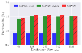
S2PNM-stat and S2PNM-dynm denote the S2PNM model with solely using static user preferences and dynamic users preferences, respectively. Figure. 2 - 5 show that S2PNM-dynm outperforms S2PNM-stat in all cases, and S2PNM (with both static and dynamic user preferences) achieves much higher accuracy than both S2PNM-dynm and S2PNM-stat. These results confirm that (1) S2PNM is effective to capture user dynamic preferences and (2) static user preferences are also necessary for predicting user future ratings without which the performance will be suboptimal. In addition, we can see that S2PNM-dynm and S2PNM have comparable results in terms of Precision@5 and HR@5, whereas S2PNM significantly outperforms S2PNM-dynm in NDCG@5. This indicates that users’ static preferences can help to put right recommendations in higher positions.
4.2.2 Effects of dictionary size
The leftmost figures of Fig. 2 - 5 show the accuracy with different dictionary sizes, i.e., varies in . In Fig. 2 (left), we set user embedding size = 50 and the number of hidden units in GRU = 32. In Fig. 3 (left), we set = 250 and = 256. As shown in the results, increasing the dictionary size can increase accuracy when varies in . This makes sense because a large dictionary can increase the capacity of S2PNM. Therefore, we choose = 1024 for the accuracy comparison.
4.2.3 Effects of GRU size
The middle figures of Fig. 2 - 5 show the recommendation accuracy with varying number of hidden units in GRU (). In Fig. 2 (middle), we set and . In Fig. 3 (middle), we set and . As shown in the results, increasing the GRU size can improve the model performance when . However, all ranking metrics dropped when , which suggests that overfitting happens with . Therefore, we choose for the accuracy comparison.
4.2.4 Effects of embedding size
The rightmost figures of Fig. 2 - 5 show the recommendation accuracy with the embedding size varying in . In Fig. 2 (right), we set and . In Fig. 3, we set and . We can see from the results that higher accuracy can be achieved with larger user embedding size, which is consistent with existing methods [43, 28]. Therefore, we choose in the following accuracy comparison although higher could further improve the performance of S2PNM.
| Method | Model | RMSE |
| SVD++ | Factorization | 0.89267 |
| TimeSVD++ | Factorization | 0.90762 |
| GLOMA | Factorization | 0.89326 |
| MRMA | Factorization | 0.89210 |
| I-AutoRec | Neural | 0.92185 |
| RRN | Neural | 0.89014 |
| NADE(2 layers) | Neural | 0.88876 |
| S2PNM, =50 | Neural | 0.87661 |
| S2PNM, =200 | Neural | 0.87386 |
| S2PNM, =300 | Neural |
4.3 Rating Prediction Comparison
4.3.1 Comparison with State-of-the-art methods
This experiment compares the rating prediction accuracy of S2PNM against state-of-the-art factorization methods [28, 29, 5, 34] and neural methods [51, 62, 68]. Note that SVD++ , GLOMA and MRMA are factorization models which assume that user preferences are static, while TimeSVD++ [29] used a time-dependent bias term to capture the temporal effects. RRN [62] and NADE [68] both leverage the neural autoregressive model to extract the patterns of how user future actions are affected by his/her historical behaviors. For S2PNM, we use a single-layer RNN with GRU units, the dimension of user embedding ranges in , and set the dictionary size as .
Table III compares the RMSE of all the methods on the Netflix prize dataset. We can see that S2PNM with = 50 can outperform SVD++[28], TimeSVD++ [29], GLOMA [5] and MRMA [34] with the rank of 300, I-AutoRec [51] and NADE [68] with 1000-dimension embeddings, RRN [62] with 300-dimension embeddings. This demonstrates that S2PNM is more effective to predict user ratings than the compared methods. In addition, compared with NADE, S2PNM achieves performance gain and over 5X efficiency improvement. The main reasons why S2PNM can improve the recommendation accuracy are: 1) the learned dictionary which maximizes the use of the GRU outputs enriches the expressive capacity of the S2PNM model, 2) the neural network-based distribution approximator that attentively reads the dictionary atoms can accurately capture the dynamic preferences of users, and 3) both the static and dynamic preferences of users are modelled by S2PNM instead of only modeling the static preferences in SVD++, GLOMA, MRMA and I-AutoRec.
4.3.2 Comparison with MRMA on different users

To understand how sequential information help in recommendation, we conduct a detailed comparison with the MRMA method which only learns static preferences of users. As shown in Fig. 6, S2PNM achieves consistent improvements () over MRMA for all kinds of users and the largest improvement is on users with less than ratings. The fact that users with less ratings benefit more from S2PNM indicates that (1) the sequential information captured by S2PNM are indeed helpful when little information of users are obtained from ratings (not enough ratings), and (2) S2PNM may be applied to address the on long-tail user issue where many existing CF methods may fail [63].
4.4 Item Ranking Comparison
4.4.1 Comparison with State-of-the-art methods
| Measures(%) | Precision@5 | HR@5 | NDCG@5 |
| SVD++ | 0.618 | 3.108 | 0.650 |
| BPR | 0.689 | 3.334 | 0.694 |
| eALS | 0.677 | 3.262 | 0.725 |
| NeuMF | 0.802 | 3.579 | 0.779 |
| RUM | 0.692 | 3.590 | 0.791 |
| SHAN | 0.764 | 3.703 | 0.759 |
| SASRec | 0.812 | 3.901 | 0.787 |
| S2PNM, =50 | 0.717 | 3.525 | 0.712 |
| S2PNM, =200 | 0.812 | 3.960 | 0.835 |
| S2PNM, =300 | 0.820 | 4.000 | 0.835 |

Here, we evaluate S2PNM in item ranking task. Differing from rating prediction experiment, this study uses = 5000 and = 256 with batch size as 128. Beside SVD++, we compare S2PNM with four ranking-based methods including BPR [46], eALS [20], NeuMF [19], RUM [9], SHAN [64] and SASREC [26]. Note that NeuMF is a neural method that is designed to utilize implicit feedback with non-linear interactions to improve performance and RUM is a state-of-the-art sequential recommendation method based on external memory network to capture the dynamic user preferences.
Table IV shows the recommendation accuracy of S2PNM and the four compared methods on the Amazon Baby Care dataset. We can see from the results that the four neural methods (NeuMF, RUM, SHAN and SASREC) significantly outperform all factorization methods (SVD++, BPR, and eALS), which confirms that neural methods are indeed more powerful than factorization methods in sequential recommendation. As shown in the table, SASREC achieved the best performance among all the compared method. However, S2PNM outperforms SASREC by 0.99%, 2.54% and 6.10% in terms of Precision5, HR5 and NDCG@5, respectively. This indicates that S2PNM can better capture the sequential interactions between users and items for more accurate recommendation.
4.4.2 Comparison with RUM on different users
As mentioned previously, S2PNM bears some similarities with RUM [9]. The main difference lies in that RUM directly combines user preferences and sequential patterns, while S2PNM translates sequential patterns to dynamic part of user preferences. Fig. 7 compares S2PNM with RUM by HR@5 (results of NDCG and Precision show the same trend thus omitted for space). It is clear that S2PNM consistently outperforms RUM for all kinds of users and the largest improvement is on users with less than ratings. This highlights the importance of translating sequence to preference, especially for sparse users that have few history in training.
| neighborhood computed at 1580-th day, movies watched during day 1580-1826 | ||||||||||
|
|
|||||||||
|
|
|||||||||
| neighborhood computed at 1826-th day, movies watched during day 1826-1860 | ||||||||||
|
|
|||||||||
|
|
|||||||||
| neighborhood computed at 1997-th day, movies watched during day 1997-2118 | ||||||||||
|
|
|||||||||
|
|
|||||||||
4.5 Qualitative Analysis
Here, a qualitative analysis is conducted to better understand the dynamic user preferences captured by S2PNM. To verify if the additive user dynamic preference captured by S2PNM can help track user preference drifts and predict user future preferences, we select the most similar neighbors using Cosine similarity given each . Then, we study the semantic meanings of the neighbors by extracting the most frequent keywords from the movie titles watched by the neighbors.
Table V presents an example for the Netflix user with id=1, and meanwhile presents the user preference drifts represented by the changes of neighbors over different periods of time. We can see from the results:
-
1.
before day 131313The elapsed day is defined as the number of days after the system’s initial date – Nov. 11th 1999., we can see that the user ids of the top 3 neighbors are: , , – all with strong interests in Lord of Rings and Star War. This suggests that user 1 prefered sci-fiction and fantasy movies, which can be verified by the most popular movies watched by user within the period (day 1580 – 1826);
-
2.
during day 1826 – 1860, user preferences shifted from sci-fiction and fantasy movies to romance and comedy movies, e.g., Absence of Malic, and crime movies, e.g., Along Came Poll. Similar patterns also occur in neighborhood: user was closer to user who favored romance and comedy movies and user who favored crime movies;
-
3.
at day 1997, the neighbors became comprehensive - user and user are fans of sci-fiction and fantasy movies, user also shows interests to romance movies, and user is interested to crime movies. Conformed with the patterns unveiled by the neighbors, user watched movies across multiple genres in the next 4 months, including fantasy movies - Lord of the Rings and Harry Potter, sci-fiction movie - Star War, romance movie - Friends, and crime movie - The Sopranos.
It is worth noting that traditional matrix factorization methods work with static user embeddings and thus cannot adjust user preferences over time. This study confirms that S2PNM can adapt automatically to the changes of user interest and thus can help adjust the predictions. We can also learn from the study that user preference drifts are complex and using simple temporal bias terms, e.g., TimeSVD++ [29], could not optimally capture these dynamic information.
5 Related Work
Many collaborative filtering works [1, 54] formulate personalized recommendation problems as matrix completion problems, of which the goal is to recover the missing entries in the rating matrix based on low-rank assumptions. In general, the attributes or preferences of a user are modeled by linearly combining item factor vectors using user-specific coefficients. And most of traditional CF solutions [48, 52, 30, 66, 46, 33, 6, 20] assume the user profiles and item attributes are static so that temporal or sequential information are ignored. Probably the most popular variants are Probabilistic Matrix Factorization (PMF) [41] and its Bayesian extension [49], which achieved robust and strong results in rating prediction. In addition to simple matrix factorization based CF models, hybrid methods have also been investigated in the literature. The Netflix Prize winners Bell et al. [3] and Koren et al. [28] utilized the combination of memory-based and matrix factorization methods to improve the recommendation accuracy. Another research line focuses on the issue of the computational efficiency, for example Mackey et al. [38] employed a Divide-Factor-Combine (DFC) framework as well as [33, 6, 58], in which the expensive task of matrix factorization is randomly divided into smaller subproblems which can be solved in parallel using arbitrary matrix factorization algorithms.
Temporal aspects in recommendation were discussed in TimeSVD++ [29]. The key innovation here lies in that TimeSVD++ introduced time-dependent bias terms to capture temporal dynamics caused by rating scale changes and popularity changes in an integrated fashion [62]. However, the features of TimeSVD++ are hand engineered similar to SVDFeature [8], which makes the model difficult to adapt to new problems due to the lack of the knowledge of the new dataset. To remedy this issue, Factorized Personalized Markov Chains (FPMC) [47] and its extension – hierarchical representation model (HRM) [59] were proposed, of which both embedded the adjacent behavior transition into the latent space. By doing so, the local patterns between items can be exploited in an end-to-end way. Beyond two-step behavior modeling, Markov chain is used for modeling sparse sequence[16]. One major issue of using Markov chains is potential state space explosion in face of different possible sequences over items.
As the revolution of deep learning, many efforts [15, 19, 36] have been made to adopt neural networks to solve the recommendation tasks, which are also mostly focused on the static collaborative filtering setting, i.e., without considering the temporal or sequential information. In specific, one of the earliest works proposed to apply Restricted Boltzmann Machines (RBM) [50] for collaborative filtering. Later, Autoencoder-based method [51] was proposed, which regards the recommendation task as a denoising problem. To exploit the ordinal nature of ratings, neural auto-regressive distribution estimator (NADE) [68] has been used to perform collaborative filtering. The above neural methods showed excellent empirical performance on popular benchmark datasets in static recommendation.
More recently, another line of emerging works employ recurrent/memory networks [22, 10, 37] to tackle the more practical task of sequential recommendation – to predict the future behavior given a user’s historical rating records. This family of the algorithms [65, 9, 25, 62, 64] can usually outperform the aforementioned Markov chain-based methods [47, 59] due to the higher model capacity. In more detail, the Dynamic REcurrent bAsket Model (DREAM) [65] embeded user historical ratings by a RNN to predict his/her future preference. And similarly the Recurrent Recommender Network (RRN) [62] proposed to employ LSTM [22] to capture the dynamics of both users and items. Complementary to the RNN-based methods, Huang et al. [25] and Ren et al. [44] alternatively adopted memory networks [13, 55] to learn the short-term patterns, together with item attributes. In the meanwhile, the Sequential Hierarchical Attention Network (SHAN) [64] and [26, 67] introduced the attention mechanism to automatically assign different influences of items in a user’s long-term set so that the dynamic properties can be captured, then relied on another attention layer to couple user sequential behavior with long-term representation.
Probably most closely related to our work is RUM [9], one of the few neural networks models for sequential recommendation. It utilized an external memory matrix to maintain item-level historical information. When making predictions, the memory of the latest interacted items in a fixed-size window (controlled by parameter ) would be attentively read out to generate an embedding as dynamic part of the user representation. However, we argue that the different sequential patterns might emerge on different timescales such that a simple first-in-first-out windowed mechanism might limit the model capacity. From the experiments, we can observe that our model outperforms state-of-the-art RUM in term of ranking prediction.
In a nutshell, this work formulates the sequential recommendation task as a supervised dictionary learning task. The proposed S2PNM method learns a dictionary to construct user dynamic preferences, which can embed user static and dynamic preferences under the same latent space, making the model very compact. Thus, S2PNM can achieve superior performance by a simple additive mechanism to fuse the static and dynamic preferences of users. To the best of our knowledge, this is the first work that translates user rating sequence into user preference via dictionary learning for sequential recommendation. The experiments on Netflix and Amazon datasets demonstrate that S2PNM can significantly outperform the state-of-the-art matrix factorization methods and neural collaborative filtering methods in the realistic setting.
6 Conclusion and Future Work
This paper proposes S2PNM – a sequence-to-preference neural machine for sequential recommendation. In particular, we propose the Seq2Pref Network for dynamic user preference modeling, which first embeds the sequential dependencies into a latent vector and then translates the dynamic preference into the latent space of user static preference using a learned dictionary. Empirical studies on multiple real-world datasets demonstrate that S2PNM can achieve significantly higher accuracy compared with state-of-the-art factorization and neural sequential recommendation methods.
One line of future work is to study pair-wise learners for S2PNM and extend S2PNM for multi-media items, whereby multi-media items such as videos and images, contains much richer semantics that reflects the interest of users. This requires the model capable of modeling auxiliary information – learn from multi-view and multi-modal data. The second future work is to introduce non-linearity when combing the static user preferences and dynamic user preferences, which may further improve the performance of the proposed method [18]. Another emerging problem is to learn the meaningful dependencies from the fragmented sequence instead of overall sequences, without sacrificing the recommendation qualities. This matters a lot for practical recommender systems. One more future direction is to explore the potential of time-aware recurrent neural networks by devising an extra loss of the RNN-based auto-regressive models to improve the performance of event-time prediction.
Acknowledgements
This work was partially supported by National Natural Science Foundation of China under Grant Nos. U19B2035 and 61972250, and National Key Research and Development Program of China under Grant Nos. 2016YFB1001003, 2018AAA0100704 and 2018YFC0830400.
References
- [1] G. Adomavicius and A. Tuzhilin. Toward the next generation of recommender systems: A survey of the state-of-the-art and possible extensions. IEEE Transactions on Knowledge and Data Engeering, 17(6):734–749, 2005.
- [2] R. Baral, S. Iyengar, T. Li, and N. Balakrishnan. Close: Contextualized location sequence recommender. In Proceedings of the 12th ACM Conference on Recommender Systems, Proceedings of the 12th ACM Conference on Recommender Systems (RecSys ’18), pages 470–474. ACM, 2018.
- [3] R. Bell, Y. Koren, and C. Volinsky. Modeling relationships at multiple scales to improve accuracy of large recommender systems. In Proceedings of the 13th ACM SIGKDD international conference on Knowledge discovery and data mining (KDD ’07), pages 95–104, 2007.
- [4] J. Bennett and S. Lanning. The netflix prize. In KDD Cup, pages 35–35, 2007.
- [5] C. Chen, D. Li, Q. Lv, J. Yan, L. Shang, and S. M. Chu. GLOMA: Embedding global information in local matrix approximation models for collaborative filtering. In Thirty-First AAAI Conference on Artificial Intelligence (AAAI ’17), pages 1295–1301, 2017.
- [6] C. Chen, D. Li, Y. Zhao, Q. Lv, and L. Shang. WEMAREC: Accurate and scalable recommendation through weighted and ensemble matrix approximation. In Proceedings of the 38th International ACM SIGIR conference on Research and Development in Information Retrieval (SIGIR ’15), pages 303–312, 2015.
- [7] T. Chen, Y. Sun, Y. Shi, and L. Hong. On sampling strategies for neural network-based collaborative filtering. In Proceedings of the 23rd ACM SIGKDD International Conference on Knowledge Discovery and Data Mining, pages 767–776, 2017.
- [8] T. Chen, W. Zhang, Q. Lu, K. Chen, Z. Zheng, and Y. Yu. Svdfeature: a toolkit for feature-based collaborative filtering. Journal of Machine Learning Research, 13:3619–3622, 2012.
- [9] X. Chen, H. Xu, Y. Zhang, J. Tang, Y. Cao, Z. Qin, and H. Zha. Sequential recommendation with user memory networks. In Proceedings of the Eleventh ACM International Conference on Web Search and Data Mining, WSDM ’18, pages 108–116, 2018.
- [10] K. Cho, B. van Merrienboer, C. Gulcehre, D. Bahdanau, F. Bougares, H. Schwenk, and Y. Bengio. Learning phrase representations using rnn encoder–decoder for statistical machine translation. In Proceedings of the 2014 Conference on Empirical Methods in Natural Language Processing (EMNLP ’14), pages 1724–1734, 2014.
- [11] J. K. Chorowski, D. Bahdanau, D. Serdyuk, K. Cho, and Y. Bengio. Attention-based models for speech recognition. In Advances in Neural Information Processing Systems (NIPS ’15), pages 577–585, 2015.
- [12] X. Glorot and Y. Bengio. Understanding the difficulty of training deep feedforward neural networks. In AISTATS ’10, pages 249–256, 2010.
- [13] A. Graves, G. Wayne, and I. Danihelka. Neural turing machines. arXiv preprint arXiv:1410.5401, 2014.
- [14] G. Guo, J. Zhang, Z. Sun, and N. Yorke-Smith. Librec: A java library for recommender systems. In UMAP Workshops, volume 4, 2015.
- [15] H. Guo, R. Tang, Y. Ye, Z. Li, and X. He. Deepfm: a factorization-machine based neural network for ctr prediction. In Proceedings of the 26th International Joint Conference on Artificial Intelligence (IJCAI’17), pages 1725–1731. AAAI Press, 2017.
- [16] R. He and J. McAuley. Fusing similarity models with markov chains for sparse sequential recommendation. In 2016 IEEE 16th International Conference on Data Mining (ICDM ’16), pages 191–200, 2016.
- [17] R. He and J. McAuley. Ups and downs: Modeling the visual evolution of fashion trends with one-class collaborative filtering. In Proceedings of the 25th International Conference on World Wide Web (WWW ’16), pages 507–517, 2016.
- [18] X. He and T.-S. Chua. Neural factorization machines for sparse predictive analytics. In Proceedings of the 40th International ACM SIGIR Conference on Research and Development in Information Retrieval, SIGIR ’17, page 355–364. Association for Computing Machinery, 2017.
- [19] X. He, L. Liao, H. Zhang, L. Nie, X. Hu, and T.-S. Chua. Neural collaborative filtering. In Proceedings of the 26th International Conference Companion on World Wide Web (WWW ’17), pages 173–182, 2017.
- [20] X. He, H. Zhang, M.-Y. Kan, and T.-S. Chua. Fast matrix factorization for online recommendation with implicit feedback. In Proceedings of the 41th International ACM SIGIR conference on Research and Development in Information Retrieval (SIGIR ’16), pages 549–558. ACM, 2016.
- [21] B. Hidasi, A. Karatzoglou, L. Baltrunas, and D. Tikk. Session-based recommendations with recurrent neural networks. In The 4th International Conference on Learning Representations (ICLR ’16), 2016.
- [22] S. Hochreiter and J. Schmidhuber. Long short-term memory. Neural computation, 9(8):1735–1780, 1997.
- [23] M. Hosseinzadeh Aghdam, N. Hariri, B. Mobasher, and R. Burke. Adapting recommendations to contextual changes using hierarchical hidden markov models. In Proceedings of the 9th ACM Conference on Recommender Systems (RecSys ’15), pages 241–244. ACM, 2015.
- [24] Y. Hu, Y. Koren, and C. Volinsky. Collaborative filtering for implicit feedback datasets. In 2008 IEEE 8th International Conference on Data Mining (ICDM ’08), pages 263–272, 2008.
- [25] J. Huang, W. X. Zhao, H. Dou, J.-R. Wen, and E. Chang. Improving sequential recommendation with knowledge-enhanced memory networks. In Proceedings of the 41th International ACM SIGIR conference on Research and Development in Information Retrieval (SIGIR ’18), pages 505–514, 2018.
- [26] W.-C. Kang and J. McAuley. Self-attentive sequential recommendation. In Proceedings of 2018 IEEE International Conference on Data Mining (ICDM’18), pages 197–206. IEEE, 2018.
- [27] D. P. Kingma and J. Ba. Adam: A method for stochastic optimization. In The 3rd International Conference on Learning Representations (ICLR ’15), 2015.
- [28] Y. Koren. Factorization meets the neighborhood: a multifaceted collaborative filtering model. In Proceedings of the 14th ACM SIGKDD international conference on Knowledge discovery and data mining (KDD ’08), pages 426–434, 2008.
- [29] Y. Koren. Collaborative filtering with temporal dynamics. In Proceedings of the 15th ACM SIGKDD international conference on Knowledge discovery and data mining (KDD ’09), pages 447–456, 2009.
- [30] Y. Koren, R. Bell, and C. Volinsky. Matrix factorization techniques for recommender systems. Computer, 42(8):30–37, 2009.
- [31] A. Kyrola, G. Blelloch, and C. Guestrin. Graphchi: Large-scale graph computation on just a PC. In The 10th USENIX Symposium on Operating Systems Design and Implementation (OSDI ’12), pages 31–46, 2012.
- [32] D. D. Lee and H. S. Seung. Algorithms for non-negative matrix factorization. In Advances in Neural Information Processing Systems (NIPS ’01), pages 556–562, 2001.
- [33] J. Lee, S. Kim, G. Lebanon, and Y. Singer. Local low-rank matrix approximation. In The 30th International Conference on Machine Learning (ICML ’13), pages 82–90, 2013.
- [34] D. Li, C. Chen, W. Liu, T. Lu, N. Gu, and S. Chu. Mixture-rank matrix approximation for collaborative filtering. In Advances in Neural Information Processing Systems (NIPS ’17), pages 477–485, 2017.
- [35] Y. Li, Y. Liang, and A. Risteski. Recovery guarantee of non-negative matrix factorization via alternating updates. In Advances in Neural Information Processing Systems (NIPS ’16), pages 4987–4995, 2016.
- [36] J. Lian, X. Zhou, F. Zhang, Z. Chen, X. Xie, and G. Sun. xdeepfm: Combining explicit and implicit feature interactions for recommender systems. In Proceedings of the 24th ACM SIGKDD International Conference on Knowledge Discovery & Data Mining (KDD’18), pages 1754–1763. ACM, 2018.
- [37] C. Ma, P. Kang, and X. Liu. Hierarchical gating networks for sequential recommendation. In Proceedings of the 25th ACM SIGKDD International Conference on Knowledge Discovery & Data Mining (KDD’19), pages 825–833, 2019.
- [38] L. W. Mackey, M. I. Jordan, and A. Talwalkar. Divide-and-conquer matrix factorization. In Advances in Neural Information Processing Systems (NIPS ’11), pages 1134–1142, 2011.
- [39] J. Mairal, F. Bach, J. Ponce, and G. Sapiro. Online dictionary learning for sparse coding. In The 26th International Conference on Machine Learning (ICML ’09), pages 689–696, 2009.
- [40] J. J. McAuley and J. Leskovec. From amateurs to connoisseurs: Modeling the evolution of user expertise through online reviews. In Proceedings of the 22nd International Conference Companion on World Wide Web (WWW ’13), pages 897–908. ACM, 2013.
- [41] A. Mnih and R. Salakhutdinov. Probabilistic matrix factorization. In Advances in Neural Information Processing Systems (NIPS ’07), pages 1257–1264, 2007.
- [42] V. Nair and G. E. Hinton. Rectified linear units improve restricted boltzmann machines. In The 27th International Conference on Machine Learning (ICML ’10), pages 807–814, 2010.
- [43] A. Paterek. Improving regularized singular value decomposition for collaborative filtering. In KDD CUP, pages 5–8, 2007.
- [44] K. Ren, J. Qin, Y. Fang, W. Zhang, L. Zheng, W. Bian, G. Zhou, J. Xu, Y. Yu, X. Zhu, et al. Lifelong sequential modeling with personalized memorization for user response prediction. In Proceedings of the 42nd International ACM SIGIR Conference on Research and Development in Information Retrieval (SIGIR’19), pages 565–574, 2019.
- [45] S. Rendle. Factorization machines with libFM. ACM Transactions on Intelligent Systems and Technology, 3(3):57:1–57:22, May 2012.
- [46] S. Rendle, C. Freudenthaler, Z. Gantner, and L. Schmidt-Thieme. Bpr: Bayesian personalized ranking from implicit feedback. In The 25th Conference on Uncertainty in Artificial Intelligence (UAI ’09), pages 452–461. AUAI Press, 2009.
- [47] S. Rendle, C. Freudenthaler, and L. Schmidt-Thieme. Factorizing personalized markov chains for next-basket recommendation. In Proceedings of the 19th International Conference on World Wide Web (WWW ’10), pages 811–820, 2010.
- [48] J. D. Rennie and N. Srebro. Fast maximum margin matrix factorization for collaborative prediction. In The 22nd International Conference on Machine Learning (ICML ’05), pages 713–719, 2005.
- [49] R. Salakhutdinov and A. Mnih. Bayesian probabilistic matrix factorization using markov chain monte carlo. In The 25th International Conference on Machine Learning (ICML ’08), pages 880–887, 2008.
- [50] R. Salakhutdinov, A. Mnih, and G. Hinton. Restricted boltzmann machines for collaborative filtering. In The 24th International Conference on Machine Learning (ICML ’07), pages 791–798, 2007.
- [51] S. Sedhain, A. K. Menon, S. Sanner, and L. Xie. Autorec: Autoencoders meet collaborative filtering. In Proceedings of the 24th International Conference on World Wide Web (WWW ’15), pages 111–112, 2015.
- [52] A. P. Singh and G. J. Gordon. Relational learning via collective matrix factorization. In Proceedings of the 14th ACM SIGKDD international conference on Knowledge discovery and data mining (KDD ’08), pages 650–658, 2008.
- [53] N. Srivastava, G. Hinton, A. Krizhevsky, I. Sutskever, and R. Salakhutdinov. Dropout: A simple way to prevent neural networks from overfitting. The Journal of Machine Learning Research, 15(1):1929–1958, 2014.
- [54] X. Su and T. M. Khoshgoftaar. A survey of collaborative filtering techniques. Advances in Artificial Intelligence, 2009.
- [55] S. Sukhbaatar, J. Weston, R. Fergus, et al. End-to-end memory networks. In Advances in Neural Information Processing Systems (NIPS ’15), pages 2440–2448, 2015.
- [56] A. van den Oord, N. Kalchbrenner, L. Espeholt, O. Vinyals, A. Graves, et al. Conditional image generation with pixelcnn decoders. In Advances in Neural Information Processing Systems (NIPS ’16), pages 4790–4798, 2016.
- [57] A. Vaswani, N. Shazeer, N. Parmar, J. Uszkoreit, L. Jones, A. N. Gomez, Ł. Kaiser, and I. Polosukhin. Attention is all you need. In Advances in Neural Information Processing Systems (NIPS ’17), pages 6000–6010, 2017.
- [58] K. Wang, W. X. Zhao, H. Peng, and X. Wang. Bayesian probabilistic multi-topic matrix factorization for rating prediction. In IJCAI ’16, pages 3910–3916, 2016.
- [59] P. Wang, J. Guo, Y. Lan, J. Xu, S. Wan, and X. Cheng. Learning hierarchical representation model for nextbasket recommendation. In Proceedings of the 38th International ACM SIGIR conference on Research and Development in Information Retrieval (SIGIR ’15), pages 403–412, 2015.
- [60] Q. Wang, H. Yin, Z. Hu, D. Lian, H. Wang, and Z. Huang. Neural memory streaming recommender networks with adversarial training. In Proceedings of the 24th ACM SIGKDD International Conference on Knowledge Discovery & Data Mining (KDD’18), pages 2467–2475, 2018.
- [61] J. Weston, S. Chopra, and A. Bordes. Memory networks, 2014.
- [62] C.-Y. Wu, A. Ahmed, A. Beutel, A. J. Smola, and H. Jing. Recurrent recommender networks. In Proceedings of the Tenth ACM International Conference on Web Search and Data Mining (WSDM ’17), pages 495–503, 2017.
- [63] H. Yin, B. Cui, J. Li, J. Yao, and C. Chen. Challenging the long tail recommendation. Proceedings of the VLDB Endowment, 5(9):896–907, 2012.
- [64] H. Ying, F. Zhuang, F. Zhang, Y. Liu, G. Xu, X. Xie, H. Xiong, and J. Wu. Sequential recommender system based on hierarchical attention networks. In Proceedings of the 27th International Joint Conference on Artificial Intelligence (IJCAI’18), 2018.
- [65] F. Yu, Q. Liu, S. Wu, L. Wang, and T. Tan. A dynamic recurrent model for next basket recommendation. In Proceedings of the 39th International ACM SIGIR conference on Research and Development in Information Retrieval (SIGIR ’16), 2016.
- [66] K. Yu, S. Zhu, J. Lafferty, and Y. Gong. Fast nonparametric matrix factorization for large-scale collaborative filtering. In Proceedings of the 32nd International ACM SIGIR conference on Research and Development in Information Retrieval (SIGIR ’09), pages 211–218, 2009.
- [67] T. Zhang, P. Zhao, Y. Liu, V. S. Sheng, J. Xu, D. Wang, G. Liu, and X. Zhou. Feature-level deeper self-attention network for sequential recommendation. In Proceedings of the 28th International Joint Conference on Artificial Intelligence (IJCAI’19), pages 4320–4326, 2019.
- [68] Y. Zheng, B. Tang, W. Ding, and H. Zhou. A neural autoregressive approach to collaborative filtering. In The 33rd International Conference on Machine Learning (ICML ’16), pages 764–773, 2016.
![[Uncaptioned image]](https://cdn.awesomepapers.org/papers/c11411f2-0420-45fc-a84a-01ed6d04a5b1/Photo_Chen.png) |
Chao Chen (M’19) is a PhD candidate in School of Electronic Information and Electrical Engineering, Shanghai Jiao Tong University, Shanghai, China. He joined IBM Research - China since May 2016, and before that he studied in department of Computer Science from Tongji University, Shanghai, China. His research interests focus on applying neural networks techniques to recommender systems. |
![[Uncaptioned image]](https://cdn.awesomepapers.org/papers/c11411f2-0420-45fc-a84a-01ed6d04a5b1/Photo_Li.png) |
Dongsheng Li (M’14) is a senior researcher with Microsoft Research Asia (MSRA), Shanghai, since February 2020. Before joining MSRA, he was a research staff member with IBM Research – China since April 2015. He is also an adjunct professor with School of Computer Science, Fudan University, Shanghai, China. He obtained Ph.D. from School of Computer Science of Fudan University, China, in 2012. His research interests include recommender systems and general machine learning applications. |
![[Uncaptioned image]](https://cdn.awesomepapers.org/papers/c11411f2-0420-45fc-a84a-01ed6d04a5b1/yanjunchi1.jpg) |
Junchi Yan (M’10) is currently an Associate Professor (PhD Advisor) with Department of Computer Science and Engineering, and AI Institute of Shanghai Jiao Tong University. He is also the co-director for the prestigious SJTU ACM Class (in charge of AI direction). Before that, he was a Senior Research Staff Member with IBM Research – China where he started his career since April 2011, and once an adjunct professor with the School of Data Science, Fudan University. His research interests are machine learning and computer vision. He serves as Associate Editor for IEEE ACCESS, (Managing) Guest Editor for IEEE Transactions on Neural Network and Learning Systems, Pattern Recognition Letters, Pattern Recognition, Vice Secretary of China CSIG-BVD Technical Committee, and on the executive board of ACM China Multimedia Chapter. He has published 40+ peer reviewed papers in top venues in AI and has filed 20+ US patents. He has once been with IBM Watson Research Center, Japan NII, and Tencent/JD AI lab as a visiting researcher. He won the Distinguished Young Scientist of Scientific Chinese and CCF Outstanding Doctoral Thesis. |
![[Uncaptioned image]](https://cdn.awesomepapers.org/papers/c11411f2-0420-45fc-a84a-01ed6d04a5b1/xiaokang.jpg) |
Xiaokang Yang (M’00-SM’04-F’19) received the B. S. degree from Xiamen University, in 1994, the M. S. degree from Chinese Academy of Sciences in 1997, and the Ph.D. degree from Shanghai Jiao Tong University in 2000. He is currently a Distinguished Professor of School of Electronic Information and Electrical Engineering, Shanghai Jiao Tong University, Shanghai, China. His research interests include visual signal processing and communication, media analysis and retrieval, and pattern recognition. He serves as an Associate Editor of IEEE Transactions on Multimedia and an Associate Editor of IEEE Signal Processing Letters. Prof. Yang is also a fellow of IEEE. |