Model Predictive Manipulation of Compliant Objects with Multi-Objective Optimizer and Adversarial Network for Occlusion Compensation
Abstract
The robotic manipulation of compliant objects is currently one of the most active problems in robotics due to its potential to automate many important applications. Despite the progress achieved by the robotics community in recent years, the 3D shaping of these types of materials remains an open research problem. In this paper, we propose a new vision-based controller to automatically regulate the shape of compliant objects with robotic arms. Our method uses an efficient online surface/curve fitting algorithm that quantifies the object’s geometry with a compact vector of features; This feedback-like vector enables to establish an explicit shape servo-loop. To coordinate the motion of the robot with the computed shape features, we propose a receding-time estimator that approximates the system’s sensorimotor model while satisfying various performance criteria. A deep adversarial network is developed to robustly compensate for visual occlusions in the camera’s field of view, which enables to guide the shaping task even with partial observations of the object. Model predictive control is utilized to compute the robot’s shaping motions subject to workspace and saturation constraints. A detailed experimental study is presented to validate the effectiveness of the proposed control framework.
Index Terms:
Robotics; Visual Servoing; Deformable Objects; Occlusion Compensation; Model Predictive ControlI Introduction
The manipulation/shaping of deformable bodies by robots is a fundamental problem that has recently attracted the attention of many researchers [1]; Its complexity has forced researchers to develop new methods in a wide range of fundamental areas that include representation, learning, planning, and control. From an applied research perspective, this challenging problem has shown great potential in various economically-important tasks such as the assembly of compliant/delicate objects [2], surgical/medical robotics [3], cloth/fabric folding [4], etc. The manipulation of compliant materials contrast with its rigid-body counterpart in that physical interactions will invariably change the object’s shape, which introduces additional degrees-of-freedom to the typically unknown objects, and hence, complicates the manipulation task. While great progress has been achieved in recent years, the development of these types of embodied manipulation capabilities is still largely considered an open research problem in robotics and control.
There are various technical issues that hamper the implementation of these tasks in real-world unstructured environments, which largely differ from implementations in ideal simulation environments (a trend followed by many recent works). Here, we argue that to effectively servo-control the shape of deformable materials in the field, a sensor-based controller must possess the following features: 1) Efficient compression of the object’s high-dimensional shape; 2) Occlusion-tolerant estimation of the objects geometry; 3) Adaptive prediction of the differential shape-motion model; Our aim in this paper is precisely to develop a new shape controller endowed with all the above-mentioned features. The proposed method is formulated under the model predictive control (MPC) framework that enables to compute shaping actions that satisfy multiple performance criteria (a key property for real engineering applications).
I-A Related Work
Many researchers have previously studied this challenging problem (we refer the reader to [5, 6] for comprehensive reviews). To servo-control the object’s non-rigid shape, it is essential to design a low-dimensional feature representation that can capture the key geometric properties of the object. Several representation methods have been proposed before, e.g., geometric features based on points, angles, curvatures, etc [7, 8]; However, due to their hard-coded nature, these methods can only be used to represent a single shaping action. Other geometric features computed from contours and centerlines [9, 10, 11] can represent soft object deformation in a more general way. Various data-driven approaches have also been proposed to represent shapes, e.g., using fast point feature histograms [12], bottleneck layers [13, 14], principal component analysis [15], etc. However, there is no widely accepted approach to compute efficient/compact feature representations for 3D shape; This is still an open research problem.
Occlusions of a camera’s field of view pose many complications to the implementation of visual servoing controllers, as the computation of (standard) feedback features requires complete visual observations of the object at all times. Many methods have been developed to tackle this critical issue, e.g. [16] used the estimated interaction matrix to handle information loss in visual servoing, yet, this method requires a calibrated visual-motor model. Coherent point drift was utilized in [17] to register the topological structure from previous sequences and to predict occlusions; However, this method is sensitive to the initial point set, further affects the registration result. A structure preserved registration method was presented in [18] to track occluded objects; This approach has good accuracy and robustness to noise, yet, its efficiency decreases with the number of points. To efficiently implement vision-based strategies in the field, it is essential to develop algorithms that can robustly guide the servoing task, even in the presence of occlusions.
To visually guide the manipulation task, control methods must have some form of model that (at least approximately) describes that how the input robot motions produce output shape changes [19]; In the visual servoing community, such differential relation is typically captured by the so-called interaction (Jacobian) matrix [20]. Many methods have been proposed to address this issue, e.g. the Broyden update rule [21] is a classical algorithm to iteratively estimate this transformation matrix [7, 22, 23]. Although these types of algorithms do not require knowledge of the model’s structure, its estimation properties are only valid locally. Other approaches with global estimation properties include algorithms based on (deep) artificial neural networks [2], optimization-based algorithms [24], adaptive estimators [25], etc. However, the majority of existing methods estimate this model based on a single performance criterion (typically, a first-order Jacobian-like relation), which limits the types of dynamic responses that the robot can achieve during a task. A multi-objective model estimation is particularly important in the manipulation of compliant materials, as their mechanical properties are rarely known in practice, thus, making hard to meet various performance requirements.
To compute the active shaping motions, most control methods only formulate the problem in terms of the final target shape and do not typically consider the system’s physical constraints. MPC represents a feasible solution to these issues, as it performs the control tasks by optimizing cost functions over a finite time-horizon rather than finding the exact analytical solution [26]; This allows MPC to compute controls that guide the task while satisfying a set of constraints, e.g., control saturation, workspace bounds, etc. Despite its valuable and flexible properties, MPC has not been sufficiently studied in the context of shape control of deformable objects.
I-B Our Contribution
To solve the above-mentioned issues, in this paper we propose a new control framework to manipulate purely-elastic objects into desired configurations. The original features of our new methodology include: 1) A parametric shape descriptor to efficiently characterize 3D deformations based on online curve/surface fitting; 2) A robust shape prediction network based on adversarial neural networks to compensate visual occlusions; 3) An optimization-based estimator to approximate the deformation Jacobian matrix and satisfy various performance constraints; 4) An MPC-based motion controller to guide the shaping motions while simultaneously solving workspace and saturation constraints.
To the best of the authors’ knowledge, this is the first time that a shape servoing controller is developed with all the functions proposed in this paper. To validate the effectiveness of our new methodology, we report a detail experimental study with a robotic platform manipulating various types of compliant objects.
II Problem Formulation
Notation: In this paper, we use the following frequently-used notation: Bold small letters, e.g., , denote column vectors, while bold capital letters, e.g., , denote matrices. Time evolving variables are denoted as , for as the discrete time instant. The matrix of ones is denoted by and the identity matrix as . represents the low triangle matrix of , and represents the Kronecker product.
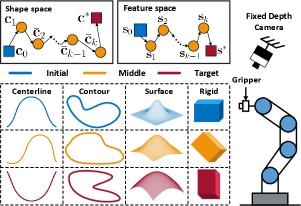
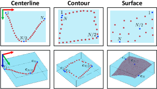
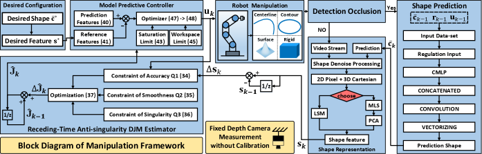
The schematic diagram of the proposed shape servoing framework is conceptually illustrated in Fig. 1. A depth camera with eye-to-hand configuration observes the shapes of elastic objects that are manipulated by the robot, see Fig. 2. We denote the 3D measurement points captured by the vision system as:
| (1) |
for as the number of points, and as the 3D coordinates of the th point, expressed in the camera frame.
II-A Feature Sensorimotor Model
Let us denote the position of the robot’s end-effector by . As the dimension of the observed points is typically very large, therefore, its direct use as a feedback signal for shape servocontrol is impractical. Therefore, an efficient controller may typically require to use some form of dimension reduction technique. To deal with this issue, we construct a feature vector , for , to represent the geometric feedback of the object. This compact feedback-like signal will be used to design our automatic 3D shape controller.
For purely elastic objects undergoing deformations, it is reasonable to model that the object configuration is only dependant on its potential energy (thus, all inertial and viscous effects are neglected from our analysis [10]). We model that is fully determined by the feedback feature vector and the robot’s position [27], i.e.: . In steady-state, the extremum expression satisfies [28]. We then define the following matrices:
| (2) |
which are useful to linearize the extremum equation (by using first-order Taylor’s series expansion) as follows:
| (3) |
for and as small changes. Note that as is satisfied, we can obtain the following motion model:
| (4) |
where represents the deformation Jacobian matrix (which depends on both the feature vector and robot position), and represents the robot’s motion control input. This model can be expressed in an intuitive discrete-time form:
| (5) |
The deformation Jacobian matrix (DJM) indicates how the robot’s action produces changes in the feedback features . Clearly, the analytical computation of requires knowledge of the physical properties and model of the elastic object and the vision system, which are difficult to obtain in practice. Thus, numerical methods are often used to approximate this matrix in real-time, which enables to perform vision-guided manipulation tasks.
In this paper, we consider a robot manipulator whose control inputs represent velocity commands (here, modelled as the differential changes ). It is assumed that can be instantaneously executed without delay [11].
Problem statement. Design a vision-based control method to automatically manipulate a compliant object into a target 3D configuration, while simultaneously compensating for visual occlusions of the camera and estimating the deformation Jacobian matrix of the object-robot system.
III Shape Representation
This section presents how online curve/surface fitting (least-squares minimization (LSM) [29] and moving least squares (MLS) [30]) is combined with a parametric shape descriptor to compute a compact vector of feedback shape features.
III-A LSM-Based Features
III-A1 Centerline and Contour Extraction
Both are expressed as a parametric curve dependent on the normalized arc-length . Then, the point can be represented as , with as the arc-length between the start point and , where and . The fitting functional is constructed as follows:
| (6) |
where the vector denotes the shape weights, specifies the fitting order, and the scalar represents a parametric regression function, which may take various forms, such as: [31]
-
•
Polynominal parameterization [32]:
(7) - •
-
•
Cox-deBoor parameterization [34]:
(9) -
•
Trigonometric parameterization [35]:
(13)
From (1) and (6), we can compute the following fitting cost function:
| (14) |
for a “tall” regression-like matrix constructed as:
| (15) |
and as a compact feedback feature vector that represents the shape. We seek to minimize (14) to obtain a feature vector that closely approximates . The solution to (14) is:
| (16) |
where it is assumed that 111In the following sections, is used to generically represent different, albeit related, functions..
III-A2 Surface Extraction
The equation of the surface is defined as follows:
| (17) |
where are the fitting order along with and direction, and is the shape weight. Same as with (14), as fitting cost function is introduced:
| (18) |
for a “augmented” regression matrix satisfying:
| (19) |
The depth vector is defiend as , and the feature vector is . The solution to the minimization of (18) that approximates is as follows:
| (20) |
For .
III-B MLS-based Feature Extraction
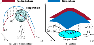
Although LSM has an efficient one-step calculation, the weights of are the same all over the variable parameters (e.g., or ). Thus, to approximate complex curves/surfaces, the fitting order needs to be increased, which may lead to over-fitting problems. To address this issue, MLS assumes that is parameter-dependent, i.e., it changes with respect to (for centerline and contour), or to (for surface). This enables MLS to represent complex shapes with a lower fitting order. A support field [36] is introduced to ensure that the value of each weight is only influenced by data points within the support field. A conceptual diagram is given in Fig. 3.
III-B1 Centerline and Contour Extraction
The parametric equation with is presented by referring to (6):
| (21) |
where the parameter-dependent weight is denoted as . The weighted square residual function is defined as:
| (22) |
where , and is the constant support field radius. The scalar function is calculated as follows [37]:
| (23) |
The function indicates the weight of relative to , decreases as increasing inside the support field. When is outside the support field, . MLS reduces into LSM when is constant. The cost (22) can be equivalently expressed in matrix form as:
| (24) |
where and are defined as follows:
| (25) | ||||
The value of that minimizes (24) is computed as follows:
| (26) |
By completing iterations along the parameter , we can compute the augmented shape features as:
| (27) |
As the dimension of (27) is very large, it is impractical to use its components as a feedback signal for control. Thus, principal components analysis (PCA) [15] is used to reduce the augmented structure (27) into a compact form where by selecting the first most significant dimensions. The feature vector is computed by vectorizing the elements of .
III-B2 Surface Extraction
The equation of the surface is constructed as:
| (28) |
where is the parameter-dependent weight related to . Algorithm 1 gives a pseudocode description of this method.
| (29) |
| (30) |
IV Shape Prediction Network
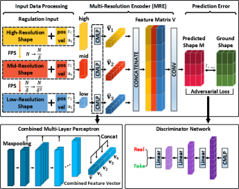
During the manipulation process, occlusions caused by obstacles or the robot itself may affect the integrity of observed shapes, and hence, the vector cannot properly describe the object’s configuration. As a solution to this critical issue, in this paper we propose an occlusion compensation shape prediction network (SPN), which is composed of a regulation input (RI), a multi-resolution encoder (MRE) and a discriminator network (DN) [40]. The proposed SPN utilizes the robot and object configurations and the active robot motions (i.e., , , ) as input to the network to predict the next instance shape, here denoted by . Fig. 4 shows the overall architecture of the SPN.
IV-A Input Data Preprocessing
As the input data to the network have different sizes, they need to be rearranged into structures with unified dimensions. To this end, is first rearranged into the matrix . Then, farthest point sampling (FPS) [41] is used to downsample to two resolutions and , for as the resolution scale. Finally, the vectors and are rearranged into the matrices and , which are similarly downsampled into mid and low resolutions as follows:
| (31) | ||||
| (32) |
Thus, three different resolutions are generated for the network, high , mid , and low , that provides a total input data of dimension . are the geometric shapes of the object under different compression sizes specified by . Thus, these three terms can describe the potential feature structure of objects. The proposed SPN aims to predict the object’s shape that results from the robots actions, under the current object-robot configuration. By using this multi-resolution data {high, mid, low}, the encoder can better learn the potential feature information of shapes.
IV-B Multi-Resolution Encoder
A combined multi-layer perceptron (CMLP) is the feature extractor of MRE, which uses the output of each layer in a MLP to form a multiple-dimensional feature vector. Traditional methods adopt the last layer of the MLP output as features, and do not consider the output of the intermediate layers, which leads to potentially losing important local information [42]. CMLP enables to make good use of low-level and mid-level features that include useful intermediate-transition information [40]. CMLP utilizes MLP to encode input data into multiple dimensions . Then, we maxpool the output of the last four layers to construct a multiple-dimensional feature vector as follows:
| (33) |
The combined feature vector is constructed as: . Three independent CMLPs map three resolutions into three individual for . Each represents the extracted potential information of each resolution. Then, the augmented feature matrix is generated by arranging its columns as , and further through 1D-convolution to obtain . Finally, the predicted next-moment shape is obtained by vectorizing . The prediction loss of MRE is:
| (34) |
where represents the ground-truth next-moment shape in the training data-set.
IV-C Discriminator Network
Generative Adversarial Network (GAN) is chosen as DN to enhance the prediction accuracy. For simplicity, we define and . We define () as the input into , while represents the true shape . is a classification network with similar structure as CMLP, constituted by serial MLP layers to distinguish the predicted shape and the real shape . We maxpool the last three layers of to obtain feature vector . Three feature vectors are concatenated into a latent vector , and then passed through the fully-connected layers followed by sigmoid-classifier to obtain the evaluation. The adversarial loss is defined as follows:
| (35) |
where , and is size of the dataset including and . The total loss of SPN is:
| (36) |
where and are the weights of and , respectively, which satisfy the condition: .
V Receding-time Model Estimation
In this paper, the objects are assumed to be manipulated by the robot slowly, thus is expected to change smoothly. For ease of presentation, we omit the arguments of and denote it as as from now on. To estimate the DJM, three indicators are considered, viz., accuracy, smoothness, and singularity. To this end, an optimization-based receding-time model (RTM) estimator is presented to estimate the changes of the Jacobian matrix, denoted by , which enables to monitor the estimation procedure. can be obtained by considering the following three constraints:
-
•
() Constraint of receding-time error [43]. As depicts the relationship between and in a local range, thus we consider the accumulated error in past moments to ensure the estimation accuracy. is the receding window size. The receding-time error is given by:
(37) The sensitivity to noise can be improved by adjusting , which helps to address the measurement fluctuations. is a constant forgetting factor giving less weight to the past observation data.
-
•
() Constraint of estimation smoothness [43]. As is assumed to be smooth, thus should be estimated smoothly to avoid sudden large fluctuations, which can be achieved by minimizing the Frobenius norm of :
(38) -
•
() Constraint of shape manipulability [44]. It evaluates the feasibility of changing the object’s shape under the current object-robot configuration:
(39) where and are the maximum and minimum eigenvalue, respectively, and . When , the object can deform isotropically in any direction. A growing indicates that the object is reaching singular (non-manipulable) configuration.
Finally, the total weighted optimization index is given by:
| (40) |
where are the weights that specify the contribution of each constraint, and which satisfy . The index (40) is then solved by using numerical optimization tools (e.g., Matlab/fmincon or Python/CasADi) to obtain and thus, iteratively update the deformation Jacobian matrix as follows: .
VI Model Predictive Controller
It is assumed that the matrix has been accurately estimated at the time instant by the RTM, such that it satisfies . Based on this model, we propose an MPC-based controller to derive the velocity inputs for the robot, while taking saturation and workspace constraints into account. Two vectors are defined as follow:
| (41) |
where and represent the predictions of and in the next periods, respectively. The vectors and denote the th predictions of and from the time instant , where , and must hold. The prediction can be calculated from the estimated Jacobian matrix by noting that is satisfied during period (which is reasonable, given the regularity of the object). This way, the predictions are computed as follows:
| (42) |
All predictions are then grouped and arranged into a single vector form:
| (43) |
In addition to and , we define the constant sequence vector that represents the desired shape feature as:
| (44) |
The cost function for the optimization of the control input is formulated as:
| (45) |
where and are the weights for the error convergence rate and the smoothness of , respectively. Two constraints are considered:
-
•
Saturation limits. In practice, robots have limits on their achievable joint speeds. These constraints are useful in soft object manipulation tasks to avoid damaging the object. Therefore, needs to be constrained:
(46) where and are the constant lower and upper bounds, respectively.
-
•
Workspace limits. Robots are also often required to operate in a confined workspace to avoid colliding with the environment. In soft object manipulation, this constraint is needed to avoid over-stretching or over-compressing the manipulated object. To this end, the following constant bounds are introduced:
(47) Similarly as in (42), the recursive structure of (47) can be obtained follows:
(48) for and defined as:
(49)
The quadratic optimization problem is formulated as follows:
| (50) |
where , and are constant matrices. Then, can be obtained by using a standard quadratic solver on (50). Finally, is calculated by the receding horizon scheme:
| (51) |
Fig. 5 presents the conceptual block diagram of the proposed framework.
Remark 2.
The proposed MPC-based technique (50) computes the robot’s shaping actions based on a performance objective and subject to system’s constraints; This approach does not require the identification of the full analytical model of the deformable object. Its quadratic optimization form enables to integrate additional metrics into the problem, e.g., rising time and overshoot.

VII Results
VII-A Experimental Setup
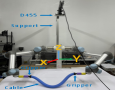
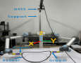
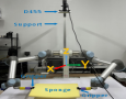
Vision-based manipulation experiments are conducted to validate our proposed framework. The experimental platform used in our study includes a fixed D455 depth sensor, a UR5 robot manipulator, and various deformable objects shown in Fig. 6. The depth sensor receives the video stream, from which it computes the 3D shapes by using the OpenCV and RealSense libraries. In our experiments, only 3 DOF of the robot manipulator are considered, therefore, the control input represents the linear velocity of the end-effector; A saturation limit of m/s, is applied for . The motion control algorithm is implemented on ROS/Python, which runs with a servo-control loop of 10 Hz. A video of the conducted experiments can be downloaded from https://github.com/JiamingQi-Tom/experiment_video/raw/master/paper4/video.mp4
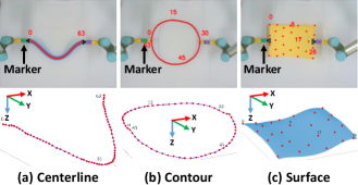
The proposed shape extraction algorithm is depicted in Fig. 7. The RGB image from the camera is transformed into HSV and combined with mask processing to obtain a binary image. is utilized with FPS to extract a fixed number of object points. The point on the centerline closest to the gripper’s green marker is chosen to sort the centerline along the cable. Then we obtain the 3D shapes by using the RealSense sensor and checking its 2D pixels. We adopt the method in [11] to compute the object’s contour. A surface is obtained in the similar way to the centerline, i.e., by sorting points from top to bottom, and from left to right. As 2D pixels and 3D points have a one-to-one correspondence in a depth camera, thus, our extraction method improves the robustness to measurement noise and is simpler than traditional point cloud processing algorithms.
| Centerline | Contour | Surface / Rigid | |
| Method | LSM | MLS | MLS |
| Support Radius | N/A | ||
| PCA | N/A | ||
| Fitting order | |||
| Basis-Function | Bernstein | Trigonometric | Polynominal |
| Numbers |
VII-B Online Fitting of the Parametric Shape Representation
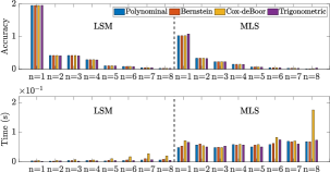
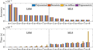
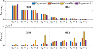
In this section, ten thousand samples of centerlines, contours and surfaces with , respectively, are collected by commanding the robot to manipulate the objects, whose configuration is then captured by a depth sensor. Such shaping actions are shown in Fig. 8, and visualized in the accompanying multimedia attachment. This data is used to evaluate the performance (viz. its accuracy and computation time) of our representation framework. For that, we calculate the average error between the feedback shape and the reconstructed shape as follows . The computation time is defined as the average of the overall processing time of all sample data among each method.
Fig. 9 shows that the larger the scalars are, the better the fitting accuracy of LSM and MLS is. MLS fits better than LSM under the same condition, as MLS calculates the independent weight while LSM assumes that each node has the same weight. MLS works better in fitting contour because the parametric curve may not be continuous in the end corner, thus, the equal weight assumption of LSM is not suitable here. As the number of data points for surface is , it does not satisfy the condition for higher order fitting models (e.g., ), thus, we only use . The results show that MLS performs better than LSM in the surface representation; Interestingly, MLS obtains satisfactory performance even with . Fig. 9 also shows that larger will also increase the computation time. MLS has a more noticeable increase, as it calculates the weights of all nodes while LSM calculates them once. The trigonometric approach is the fastest, polynomial and Bernstein follow, while Cox-deBoor is the slowest with the most iterative operations. The above analysis verifies the effectiveness of the proposed extraction framework, which can represent objects with a low-dimensional feature. Details of the curve fitting configuration is given in Table. I.
VII-C Occlusion-Robust Prediction of Object Shapes
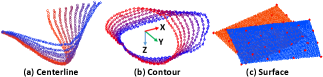
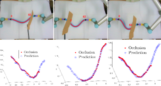
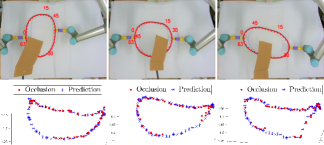
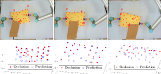
The data collected in Section VII-B is used to evaluate our proposed SPN. 80% of the data is used as the training set, and the remaining 20% of the data is used to test the trained network. We set for the centerline, contour, and surface parametrization. SPN is built using PyTorch and trained by an ADAM optimizer with a batch size of 500, and the initial learning rate set to 0.0001. RELU activation and batch normalization are adopted to improve the network’s performance. In this validation test, the robot deforms the objects with small babbling motions while a cardboard sheet covers parts of objects. Fig. 10 shows that SPN can predict and provide relatively complete shapes for the three types of manipulated objects. The accompanying video demonstrates the performance of this method.
VII-D Estimation of the Sensorimotor Model
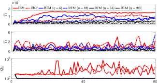
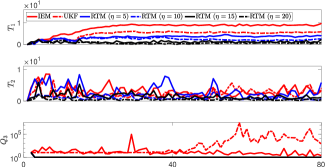
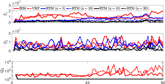
This section aims to evaluate RTM (40) that approximates the deformation Jacobian matrix; The performance of the RTM estimator is compared with the interaction matrix estimator (IEM) in [15], and the unscented Kalman filter (UKF) in [31]. To this end, we introduce two metrics, i.e., and , to quantitatively compare performances of these algorithms:
| (53) |
where is the approximated shape feature that is computed based on the control actions. Fig. 11 shows that RTM with provides the best performance for among the methods; This means that constraint (37) enables RTM to learn from past data by adjusting . Small values of reflect that RTM accurately predicts the differential changes induced by the DJM; This means that constraint (38) helps to compute a smooth matrix . As the proposed method incorporates the constraint (39), thus, RTM can prevent singularities in the estimation of the Jacobian matrix, while IEM and UKF are prone to reach ill-conditioned estimations. We use RTM with in the following sections.
VII-E Automatic Shape Servoing Control
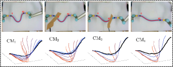
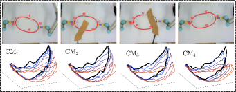
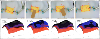
This section conducts four automatic manipulation experiments, labeled as Exp1, Exp2, Exp3, and Exp4, respectively. The target contour is obtained from previous demonstrations of the manipulation task, which ensures its reachability. A cardboard sheet is manually placed over the object to produce (partial) occlusions and test the robustness of our algorithm. The estimation methods in [15] and [31] are compared with the proposed receding-time model with MPC ( and ). We label these methods as , and each method has been optimized to achieve a balance of stability, convergence, and responsiveness.
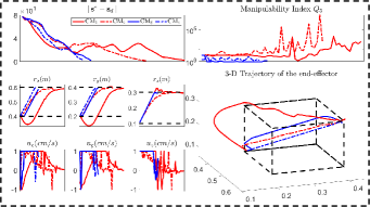
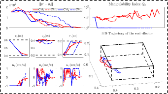
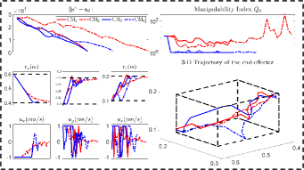
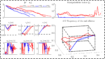
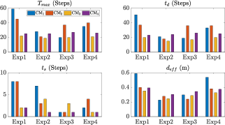
In addition to the feedback shape error , we also compare (i.e., the number of steps from start to finish), (the steps from to 10% of this value), (the steps from 10% to the threshold value), and (the total moving distance of the end-effector), [11, 23]. Fig. 12 shows the shaping motions of the manipulated objects toward the desired configuration (black curve), with the cardboard blocking the view at various instances. The results demonstrate that SPN can predict the object’s shape during occlusions and feed it back to the controller to enforce the shape servo-loop; This results in the objects being gradually manipulated towards the desired configuration. The error norm plots in Fig. 13 shows that provides the best control performance for the error minimization, with as the second-best, and and showing similar performance. A higher is helpful for feature prediction, yet, since we assume that is constant in the window period , it may lead to inaccurate predictions and even wrong manipulation of objects. Therefore, should be chosen according to the performance requirements of the system.
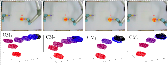
From the plots in Fig. 13, we can see RTM with provides the smallest value, which validates that RTM can enhance the manipulation feasibility and avoid shapes falling into the singular configurations. The black dashed lines represent the workspace constraints of , on which we can see the end-effector’s trajectories in the Cartesian coordinate system; The results show that and remain within the workspace, while and may violate this constraint. Due to the adopted input saturation in our platform, all four methods can satisfy the control saturation constraint. Exp4 shows that our method has good universality, not only for the shape control, but also for traditional rigid object positioning.
A performance comparison of these experiments is given in Fig. 14. The results illustrate that our proposed shape servoing framework achieves the best performance relative to the manipulation speed , response speed , convergence speed , and motion distance .
VIII Conclusions
In this paper, we present an occlusion-robust shape servoing framework to control shapes of elastic objects into target configurations, while considering workspace and saturation constraints. A low-dimensional feature extractor is proposed to represent 3D shapes based on LSM and MLS. A deep neural network is introduced to predict the object’s configuration subject to occlusions, and feed it to the shape servo-controller. A receding-time model estimator is designed to approximate the deformation Jacobian matrix with various constraints such as accuracy, smoothness, singularity. The conducted experiments validate the proposed methodology with multiple unstructured shape servoing tasks in visually occluded situations and with unknown deformation models.
However, there are some limitations in our framework. For example, as the support field radius is constant (i.e., it does not adjust with dynamic shapes), the computed representation lacks flexibility. Also, the SPN needs to obtain substantial offline training data to properly work, which might pose complications in practice. Note that our method may not accurately shape objects with negligible elastic properties (e.g., fabrics, food materials, etc). Future work include the incorporation of shape reachability detection into the framework in order to determine the feasibility of a given shaping task beforehand.
References
- [1] J. Zhu, A. Cherubini, C. Dune, D. Navarro-Alarcon, F. Alambeigi, D. Berenson, F. Ficuciello, K. Harada, X. Li, J. Pan, et al., “Challenges and outlook in robotic manipulation of deformable objects,” arXiv preprint arXiv:2105.01767, 2021.
- [2] X. Li, X. Su, and Y.-H. Liu, “Vision-based robotic manipulation of flexible pcbs,” IEEE/ASME Transactions on Mechatronics, vol. 23, no. 6, pp. 2739–2749, 2018.
- [3] L. Cao, X. Li, P. T. Phan, A. M. H. Tiong, H. L. Kaan, J. Liu, W. Lai, Y. Huang, H. M. Le, M. Miyasaka, et al., “Sewing up the wounds: A robotic suturing system for flexible endoscopy,” IEEE Robotics & Automation Magazine, vol. 27, no. 3, pp. 45–54, 2020.
- [4] Z. Hu, P. Sun, and J. Pan, “Three-dimensional deformable object manipulation using fast online gaussian process regression,” IEEE Robotics and Automation Letters, vol. 3, no. 2, pp. 979–986, 2018.
- [5] J. Sanchez, J.-A. Corrales, B.-C. Bouzgarrou, and Y. Mezouar, “Robotic manipulation and sensing of deformable objects in domestic and industrial applications: a survey,” Int. J. of Rob. Res., 2018.
- [6] H. Yin, A. Varava, and D. Kragic, “Modeling, learning, perception, and control methods for deformable object manipulation,” Science Robotics, vol. 6, no. 54, 2021.
- [7] D. Navarro-Alarcon, Y.-H. Liu, J. G. Romero, and P. Li, “Model-free visually servoed deformation control of elastic objects by robot manipulators,” IEEE Transactions on Robotics, vol. 29, no. 6, pp. 1457–1468, 2013.
- [8] D. Navarro-Alarcon, Y.-h. Liu, J. G. Romero, and P. Li, “On the visual deformation servoing of compliant objects: Uncalibrated control methods and experiments,” The International Journal of Robotics Research, vol. 33, no. 11, pp. 1462–1480, 2014.
- [9] H. Wang, B. Yang, J. Wang, X. Liang, W. Chen, and Y.-H. Liu, “Adaptive visual servoing of contour features,” IEEE/ASME Transactions on Mechatronics, vol. 23, no. 2, pp. 811–822, 2018.
- [10] D. Navarro-Alarcon and Y.-H. Liu, “Fourier-based shape servoing: a new feedback method to actively deform soft objects into desired 2-d image contours,” IEEE Transactions on Robotics, vol. 34, no. 1, pp. 272–279, 2017.
- [11] J. Qi, G. Ma, J. Zhu, P. Zhou, Y. Lyu, H. Zhang, and D. Navarro-Alarcon, “Contour moments based manipulation of composite rigid-deformable objects with finite time model estimation and shape/position control,” IEEE/ASME Transactions on Mechatronics, 2021.
- [12] Z. Hu, T. Han, P. Sun, J. Pan, and D. Manocha, “3-d deformable object manipulation using deep neural networks,” IEEE Robotics and Automation Letters, vol. 4, no. 4, pp. 4255–4261, 2019.
- [13] J. Qi, G. Ma, P. Zhou, H. Zhang, Y. Lyu, and D. Navarro-Alarcon, “Towards latent space based manipulation of elastic rods using autoencoder models and robust centerline extractions,” Advanced Robotics, vol. 36, no. 3, pp. 101–115, 2022.
- [14] P. Zhou, J. Zhu, S. Huo, and D. Navarro-Alarcon, “LaSeSOM: A latent and semantic representation framework for soft object manipulation,” IEEE Robotics and Automation Letters, vol. 6, no. 3, pp. 5381–5388, 2021.
- [15] J. Zhu, D. Navarro-Alarcon, R. Passama, and A. Cherubini, “Vision-based manipulation of deformable and rigid objects using subspace projections of 2d contours,” Robotics and Autonomous Systems, vol. 142, p. 103798, 2021.
- [16] N. Cazy, P.-B. Wieber, P. R. Giordano, and F. Chaumette, “Visual servoing when visual information is missing: Experimental comparison of visual feature prediction schemes,” in 2015 IEEE International Conference on Robotics and Automation (ICRA). IEEE, 2015, pp. 6031–6036.
- [17] T. Tang, C. Wang, and M. Tomizuka, “A framework for manipulating deformable linear objects by coherent point drift,” IEEE Robotics and Automation Letters, vol. 3, no. 4, pp. 3426–3433, 2018.
- [18] T. Tang and M. Tomizuka, “Track deformable objects from point clouds with structure preserved registration,” The International Journal of Robotics Research, p. 0278364919841431, 2018.
- [19] D. Navarro-Alarcon, J. Qi, J. Zhu, and A. Cherubini, “A lyapunov-stable adaptive method to approximate sensorimotor models for sensor-based control,” Frontiers in Neurorobotics, vol. 14, 2020.
- [20] F. Chaumette and S. Hutchinson, “Visual servo control, part I: Basic approaches,” IEEE Robotics and Automation Magazine, vol. 13, no. 4, pp. 82–90, 2006.
- [21] K. Hosoda and M. Asada, “Versatile visual servoing without knowledge of true jacobian,” in Proceedings of IEEE/RSJ International Conference on Intelligent Robots and Systems (IROS’94), vol. 1. IEEE, 1994, pp. 186–193.
- [22] F. Alambeigi, Z. Wang, R. Hegeman, Y.-H. Liu, and M. Armand, “Autonomous data-driven manipulation of unknown anisotropic deformable tissues using unmodelled continuum manipulators,” IEEE Robotics and Automation Letters, vol. 4, no. 2, pp. 254–261, 2018.
- [23] R. Lagneau, A. Krupa, and M. Marchal, “Active deformation through visual servoing of soft objects,” in 2020 IEEE International Conference on Robotics and Automation (ICRA). IEEE, 2020, pp. 8978–8984.
- [24] Lagneau, K. Romain, M. Alexandre, and Maud, “Automatic shape control of deformable wires based on model-free visual servoing,” IEEE Robotics and Automation Letters, vol. 5, no. 4, pp. 5252–5259, 2020.
- [25] L. Han, H. Wang, Z. Liu, W. Chen, and X. Zhang, “Visual tracking control of deformable objects with a fat-based controller,” IEEE Transactions on Industrial Electronics, 2021.
- [26] A. Hajiloo, M. Keshmiri, W.-F. Xie, and T.-T. Wang, “Robust online model predictive control for a constrained image-based visual servoing,” IEEE Transactions on Industrial Electronics, vol. 63, no. 4, pp. 2242–2250, 2015.
- [27] H. Wakamatsu and S. Hirai, “Static modeling of linear object deformation based on differential geometry,” The International Journal of Robotics Research, vol. 23, no. 3, pp. 293–311, 2004.
- [28] M. Yu, H. Zhong, and X. Li, “Shape control of deformable linear objects with offline and online learning of local linear deformation models,” arXiv preprint arXiv:2109.11091, 2021.
- [29] H. Abdi et al., “The method of least squares,” Encyclopedia of Measurement and Statistics. CA, USA: Thousand Oaks, 2007.
- [30] P. Lancaster and K. Salkauskas, “Surfaces generated by moving least squares methods,” Mathematics of computation, vol. 37, no. 155, pp. 141–158, 1981.
- [31] J. Qi, W. Ma, D. Navarro-Alarcon, H. Gao, and G. Ma, “Adaptive shape servoing of elastic rods using parameterized regression features and auto-tuning motion controls,” arXiv preprint arXiv:2008.06896, 2020.
- [32] K. Smith, “On the standard deviations of adjusted and interpolated values of an observed polynomial function and its constants and the guidance they give towards a proper choice of the distribution of observations,” Biometrika, vol. 12, no. 1/2, pp. 1–85, 1918.
- [33] G. G. Lorentz, Bernstein polynomials. American Mathematical Soc., 2013.
- [34] I. J. Schoenberg, Cardinal spline interpolation. SIAM, 1973.
- [35] M. J. D. Powell et al., Approximation theory and methods. Cambridge university press, 1981.
- [36] W. Y. Tey, N. A. Che Sidik, Y. Asako, M. W Muhieldeen, and O. Afshar, “Moving least squares method and its improvement: A concise review,” Journal of Applied and Computational Mechanics, vol. 7, no. 2, pp. 883–889, 2021.
- [37] H. Zhang, C. Guo, X. Su, and C. Zhu, “Measurement data fitting based on moving least squares method,” Mathematical Problems in Engineering, vol. 2015, 2015.
- [38] J. C. Mason and D. C. Handscomb, Chebyshev polynomials. CRC press, 2002.
- [39] R. T. Farouki, “Legendre–bernstein basis transformations,” Journal of Computational and Applied Mathematics, vol. 119, no. 1-2, pp. 145–160, 2000.
- [40] Z. Huang, Y. Yu, J. Xu, F. Ni, and X. Le, “Pf-net: Point fractal network for 3d point cloud completion,” in Proceedings of the IEEE/CVF Conference on Computer Vision and Pattern Recognition, 2020, pp. 7662–7670.
- [41] X. Yan, C. Zheng, Z. Li, S. Wang, and S. Cui, “Pointasnl: Robust point clouds processing using nonlocal neural networks with adaptive sampling,” in Proceedings of the IEEE/CVF Conference on Computer Vision and Pattern Recognition, 2020, pp. 5589–5598.
- [42] C. R. Qi, H. Su, K. Mo, and L. J. Guibas, “Pointnet: Deep learning on point sets for 3d classification and segmentation,” in Proceedings of the IEEE conference on computer vision and pattern recognition, 2017, pp. 652–660.
- [43] H. Mo, B. Ouyang, L. Xing, D. Dong, Y. Liu, and D. Sun, “Automated 3-d deformation of a soft object using a continuum robot,” IEEE Transactions on Automation Science and Engineering, 2020.
- [44] K. M. Lynch and F. C. Park, Modern robotics. Cambridge University Press, 2017.
![[Uncaptioned image]](https://cdn.awesomepapers.org/papers/2adc8720-8bfc-4ff0-baae-dbc90f557330/Tom.jpg) |
Jiaming Qi received the M.Sc. in integrated circuit engineering from Harbin Institute of Technology, Harbin, China, in 2018. In 2019, he was a visiting PhD student at The Hong Kong Polytechnic University. He is currently pursuing the Ph.D. degree with control science and engineering, Harbin Institute of Technology, Harbin, China. His current research interests include data-driven control for soft object manipulation, visual servoing, robotics and control theory. |
![[Uncaptioned image]](https://cdn.awesomepapers.org/papers/2adc8720-8bfc-4ff0-baae-dbc90f557330/Lidongyu.png) |
Dongyu Li (Member, IEEE) received the B.S. and Ph.D. degree in control science and engineering, Harbin Institute of Technology, China, in 2016 and 2020. He was a joint Ph.D. student with the Department of Electrical and Computer Engineering, National University of Singapore from 2017 to 2019, and a research fellow with the Department of Biomedical Engineering, National University of Singapore, from 2019 to 2021. He is currently an Associate Professor with the School of Cyber Science and Technology, Beihang University, China. His research interests include networked system cooperation, adaptive systems, and robotic control. |
![[Uncaptioned image]](https://cdn.awesomepapers.org/papers/2adc8720-8bfc-4ff0-baae-dbc90f557330/Gaoyufeng.png) |
Yufeng Gao (Student Member, IEEE) received his bachelor of engineering and bachelor of economics degrees from Wuhan University of Technology and Wuhan University, China, both in 2016. And he received the Ph.D. degree in control science and engineering, Harbin Institute of Technology, China, in 2021. He was a joint Ph.D. student with the Chair of Automatic Control Engineering, Technical University of Munich, Germany, from 2018 to 2019. His current research interests include spacecraft system modeling, control and optimization. |
![[Uncaptioned image]](https://cdn.awesomepapers.org/papers/2adc8720-8bfc-4ff0-baae-dbc90f557330/Jeffery.png) |
Peng Zhou (Student Member, IEEE) was born in China. He received the M.Sc. degree in software engineering from the School of Software Engineering, Tongji University, Shanghai, China, in 2017 and is currently pursuing his the Ph.D. degree in mechanical engineering at The Hong Kong Polytechnic University, Kowloon, Hong Kong. His research interests include deformable object manipulation, motion planning and robot learning. |
![[Uncaptioned image]](https://cdn.awesomepapers.org/papers/2adc8720-8bfc-4ff0-baae-dbc90f557330/x30.png) |
David Navarro-Alarcon (Senior Member, IEEE) received the Ph.D. degree in mechanical and automation engineering from The Chinese University of Hong Kong (CUHK), Shatin, Hong Kong, in 2014. From 2014 to 2017, he was a Postdoctoral Fellow and then a Research Assistant Professor with the CUHK T Stone Robotics Institute. Since 2017, he has been with The Hong Kong Polytechnic University, Hong Kong, where he is currently an Assistant Professor with the Department of Mechanical Engineering, and the Principal Investigator of the Robotics and Machine Intelligence Laboratory. His current research interests include perceptual robotics and control theory. |