Model-Agnostic and Diverse Explanations for Streaming Rumour Graphs
Abstract
The propagation of rumours on social media poses an important threat to societies, so that various techniques for rumour detection have been proposed recently. Yet, existing work focuses on what entities constitute a rumour, but provides little support to understand why the entities have been classified as such. This prevents an effective evaluation of the detected rumours as well as the design of countermeasures. In this work, we argue that explanations for detected rumours may be given in terms of examples of related rumours detected in the past. A diverse set of similar rumours helps users to generalize, i.e., to understand the properties that govern the detection of rumours. Since the spread of rumours in social media is commonly modelled using feature-annotated graphs, we propose a query-by-example approach that, given a rumour graph, extracts the most similar and diverse subgraphs from past rumours. The challenge is that all of the computations require fast assessment of similarities between graphs. To achieve an efficient and adaptive realization of the approach in a streaming setting, we present a novel graph representation learning technique and report on implementation considerations. Our evaluation experiments show that our approach outperforms baseline techniques in delivering meaningful explanations for various rumour propagation behaviours.
keywords:
explainable rumour detection , data stream , social networks , graph embedding1 Introduction
Rumours on social media are an increasingly critical issue, threatening societies at a global scale. They fuel misinformation campaigns, reduce the credibility of news outlets, and potentially affect the opinions and, hence, actions of large parts of a society. The mechanisms for content sharing and user engagement that form the basis of most social media platforms foster the propagation, amplification, and reinforcement of rumours in graph-based propagation structures [1, 2, 3]. Fig. 1 illustrates such a propagation structure for a rumour that emerged about the Las Vegas shooting in 2017, which attracted millions of engagements on Twitter and news websites.

With rumours emerging as a worldwide phenomenon, various techniques for their detection have been proposed [4, 2, 5]. However, existing techniques focus on identifying what entities are part of a rumour structure, but provide little support for explaining the obtained results [6]. Especially the increasing popularity of methods for rumour detection based on deep learning, which exploit latent features, calls for explanations on why certain entities have been classified as a rumour. Such explanations are important for various reasons: (1) they enable an evaluation of the detected rumours and, hence, serve to assess the accuracy of rumour detection techniques; (2) they outline opportunities for improving the models adopted by the detection techniques; and (3) they enable users to devise and implement countermeasures that slow down and prevent the spread of rumours in the future.
Explanations of rumours may be based on different paradigms. Since rumours are shared by humans, it is difficult to extract discrete rules to serve as explanations, though [7]. Feature-based explanations, in turn, cannot capture the graph-based propagation structures of rumours [8]. Also, counter-factual approaches are not suited to understand why entities are classified as being part of a rumour, due to their focus on features that may change the result [9]. As such, explanations shall be based on a set of related examples, which enable users to generalize their properties [10]. For a rumour represented as a graph, the explanation is then given in terms of related subgraphs of rumours detected in the past.
However, existing example-based explanation methods are still limited by easily overlooked assumptions. First, it is often assumed that the underlying model is stable over time. In practice, ML models are routinely retrained to react to changes in the overall environment and to changes in users’ features. Explanations are often generated by a model-specific approach to identify the decision boundary of a specific model [11]; and thus, become obsolete quickly when the model changes. Second, it is often assumed that there is no constraint on model access and complexity. Most of existing works generate synthetic data samples and calling the model evaluation on these samples repeatedly to identify the decision boundary to find most similar ones to the original input. However, the model is not always available for such evaluation calls (e.g. software and hardware requirements) and can be very costly in practice (e.g. some models might take minutes, if not hours, to complete a prediction) [12].
To tackle these issues, we follow a model-agnostic approach to generate examples that are applicable to different types of models. In particular our approach works generally well with various problems and domains and is free from model access requirements. The performance of existing model-specific approaches are not generalized to other settings and even change considerably with a small of change of experimental setups [12]. Moreover, our approach is not limited to a single example as in many previous works [9], but include diverse examples to increase the likelihood of returning at least one option that matches the user’s true interest. Especially, our approach is free of model bias, which can still happen in many modern ML models [13, 14].
A realization of example-based explanations for rumour detection faces diverse challenges. First, social media platforms are highly dynamic. The characteristics of rumours evolve over time, hence explanations are instance-specific. Second, rumours on social media materialize along multiple modalities, making traditional textual analysis insufficient [7]. For example, a rumour may be characterized by the relations between users and their interactions, not only by some textual content. Third, the representation of rumours as graphs induces computational challenges. It is intractable to query the respective graph structures directly [15].
In this paper, we address the above challenges and derive explanations for rumours with a query-by-example approach. Given a rumour graph, it extracts the subgraphs of past rumours that are most useful to explain the rumour, thereby achieving instance-specific explanations. By adopting a model based on feature-annotated graphs, diverse modalities can be incorporated. Moreover, we present a novel graph representation learning technique, which enables us to derive explanations efficiently in a streaming setting. More specifically, our contributions can be summarised as follows:
-
•
We define the problem of example-based explanation for rumour detection. This is the first formulation of explanations for dynamic, graph-based rumours.
-
•
We provide a framework to address the explanation problem. Given a rumour, we show how to score the utility of subgraphs of past rumours and select the most useful ones.
-
•
We design a graph representation learning technique to enable an efficient computation of explanations.
-
•
We outline how the efficiency and robustness can be increased by indexing and caching schemes.
-
•
We propose an adaptation mechanism to concept drifts, i.e. when new rumour patterns emerge and are different from past rumour examples.
We further report on evaluation experiments with synthetic and real-world data. We show that our approach delivers meaningful explanations for various rumour propagation behaviours. Compared to baseline techniques, selection of explanations with our approach is faster, while the runtime for graph similarity scoring improves by up to four orders of magnitude. Our approach also accumulates more than higher utility of explanations when a large number of rumours are detected and streamed into the system.
In the remainder, § 2 summarizes related work, before § 3 introduces a graph-based model for our work. The problem of example-based explanations for rumour detection and our general approach for it are introduced in § 4. We first clarify the utility scoring and selection of subgraphs in § 5, before realizing these steps based on graph embeddings in § 6 and presenting further optimizations in § 7. We report on experiment results in § 8, before we conclude in § 9.
2 Related Work
Explainable rumour detection. Most existing approaches to rumour detection neglect the question why certain entities have been classified as a rumour. For this reason, techniques from the field of explainable machine learning have been adopted recently. However, explainable rumour detection focuses on pinpointing specific features that explain the detection results [6]. Also, for rumour detection based on deep learning, attention mechanisms and gradient activation maps have been employed to explain the latent features used in the detection [16]. However, understanding the structure of rumours turned out to be more important than understanding the detection itself [17, 18, 19, 20]. Due to the graph-based propagation structures of rumours, explanations solely based on features insufficient [21, 22, 23, 24].
Recently, approaches to construct graph-based explanations using graph neural networks have been proposed [25, 3, 26, 27, 28]. However, the explanation is still given in terms of gradient footprints of the deep learning model rather than the characteristics of the rumour itself. Also, the explanation technique depends on the deep learning model and, hence, cannot be generalised to other detection techniques.
We go beyond the state of the art by considering the detection technique as a black-box and by providing subgraphs of related rumours as explanations. We later show empirically that such explanations have a high discriminating power.
Computational explanations. Various paradigms to explain computational results have been studied in the literature, including interpretable models, rule-based explanations, counterfactuals, and feature-based explanations [29]. Interpretable models enable a direct inspection of the factors that govern some computation, e.g., regressions, decision trees, generalized additive models, and Bayesian networks. For example, the weights learned in a linear regression and the path taken in a decision tree can directly be interpreted by a user. However, such interpretable models are not sufficiently expressive to capture the structure of rumours.
As argued above, explanations based on examples are most suited in the context of rumour detection. The reason being that rumours involve human perception, which is difficult to capture with discrete rules [7], whereas feature-based approaches fail to capture the graph-based structures of rumour propagation [8]. Counter-factual explanations, in turn, focus on features that may change the result of rumour detection rather than the features that led to the detection result in the first place [9]. While synthetic examples have the advantage of gradient optimisation [30] to generate them, real examples have the benefits of acting as case studies to convince decision makers in critical applications such as healthcare and social informatics [31].
Similar to example-based explanations based on subgraphs, as targetted in our work, exemplary contextual information, such as user comments, may be extracted to explain detected rumours [8]. However, such contextual information tends to be subjective and provides limited insight on the rumour as a whole. By extracting subgraphs of past rumours, our approach supports a more comprehensive assessment of the properties that characterize a rumour.
Subgraph querying. Our work is orthogonal to graph search. This is because the subgraphs that serve as explanations do not necessarily participate in the prediction of the rumour of interest. Even if the subgraphs and the considered rumour are of similar structure (and they are close in the embedding space), it is not obvious to what extent the detection technique applied the same reasoning and which features influenced the classification as a rumour [2]. Thereon, we formulate a subgraph selection problem that maximises a notion of explanation utility, which incorporates both similarity and diversity of the respective subgraphs.
3 Model
Below, we introduce the formal model adopted in our work, which is also summarized in Table 1.
Multi-modal Social Graph (MSG). To capture social media data, we adopt the notion of a multi-modal social graph (MSG). It is an undirected graph with entities and relations , where are all subsets of of size two [32].
Each entity and relation has a type called modality. Formally, with as a set of pre-defined entity modalities, we define a type function that maps each entity to a modality. An entity represents an instance of its modality. This model extends naturally to a streaming setting, where the set of entities is extended over time, but the set of modalities is fixed. The modality of a relation is derived directly from the modalities of the entities, and captured by a type function with being all subsets of of size two. It is defined as . For brevity, we write for either type function, when the domain is clear, and define as the set of all entity and relation modalities.
Each entity or relation can be associated with a vector of features of its modality (aka intrinsic characteristics of the modality), such as language structures and lexical features of a social post [6]. These features often capture rumour signals in a social graph. In our model, we incorporate such features by a set of functions , where assigns an -dimensional feature vector to each element of modality .
Social graphs can capture different types of social networks [33]. In the remainder, we use the case of Twitter for illustration purposes. Then, the entities of an MSG are of the modalities user, tweet, hashtag, or link. Edges capture the relations between entities, e.g., that a user created a tweet or that a link was referred to in a tweet.
| Notation | Description |
|---|---|
| A set of modalities | |
| All possible values of modalities | |
| A multi-modal social graph (MSG) | |
| An explanation of rumour subgraphs | |
| The utility of an explanation | |
| The modality of an entity | |
| Embedding of an entity | |
| Embedding of a rumour subgraph |
Rumours. For the purpose of this paper, we largely abstract from the specifics of techniques for rumour detection (except in our evaluation experiments). That is, we assume that for a given multi-modal social graph, a rumour detector identifies rumours as subgraphs of the MSG. Moreover, in a streaming setting, the MSG is extended over time by the addition of entities and edges, so that also the rumour detector constructs sets of rumours over time.
4 Problem Statement and Approach
We first explain the intuition of example-based explanations under a graph-based model by means of an example in § 4.1. Then, we present a formal statement of example-based explanations in § 4.2 and outlined our general framework to address this problem in § 4.3.
4.1 Intuition of Example-based Explanations
Consider the example given in Fig. 2. Here, a given rumour (top left) includes several entities and relations, including specific users, tweets, a hashtag, and a linked article, each being assigned further features. For example, the first user has 10K followers and the relation between the two users is marked as a friendship link that has been established one day ago. The relation between two tweets indicates a retweet with a certain time difference (1 hour), while the hashtag has the number of mentions (1M) as a feature.
Fig. 2 also shows previously detected rumours (top right), each differing in the structure and the associated features. Those that are similar to the rumour of interest may serve as explanations of rumour detection, as they enable users to generalize from the different structures and understand the general characteristics of the detected rumours. For example, in Fig. 2, users can deduce a pattern in the rumours that is given as a subgraph of a famous user (10k followers) with a new friend (1 day friendship relation), who posts a tweet that links to an old article (one year ago), which was quickly retweeted by the new friend.

Extracting a set of related rumours to explain a rumour of interest enables various downstream applications, such as group attack detection, where the common subgraphs of the returned examples help to identify groups of bot and fake accounts [34]; rumour diffusion, where commonalities and differences of the examples characterize different propagation patterns [35]; and rumour source detection, where invariant features of the examples help to identifying the genesis of rumours to develop mitigation and prevention mechanism [36]. To support these applications effectively, however, the extracted examples shall meet three criteria:
-
•
Similarity: Explanations shall be given through examples that are similar to the rumour of interest. For a graph-based model, similarity search is computational challenging, though.
-
•
Diversity: Explanations shall be fair in the sense that they are not biased to one rumour structure. Information redundancy shall be avoided to provide comprehensive insights [37].
-
•
Conciseness: Explanations shall be as simple as possible, following the principle of Occam’s razor [7]. That is, smaller sets of examples shall be favoured.
4.2 Problem Formulation
The above criteria for explanations for rumour detection correspond to somewhat conflicting goals: similarity favours biased explanations; diversity favours different explanations; and conciseness favours a small number of examples and limits the amount of information. We model the trade-off between similarity and diversity and capture the desired information through a utility function that assigns a score to all possible example (i.e., subgraphs of rumours in the past). Moreover, conciseness of the explanation is captured by a dedicated parameter that limits the number of extracted examples. Based thereon, we formulate the problem addressed in this work:
Problem 1.
Given a set of rumours detected in the past , a rumour of interest , and a utility function , the problem of example-based explanations of rumour detection is to extract a set of rumours, such that:
To support explainable rumour detection efficiently and effectively, a solution to extract the subgraphs of past rumours that are most useful shall further satisfy the following requirements:
-
(R1)
Efficient computation: The utility of past rumours shall be calculated fast with a small storage cost.
-
(R2)
Incremental computation: The approach shall be applicable for a stream of detected rumours.
-
(R3)
Adaptive computation: The approach shall support efficient updates of the underlying social graph.
4.3 Solution Framework
Our framework for example-based explanations of rumour detection is illustrated in Fig. 3. As input, our framework takes a stream of detected rumours that are returned by some black-box detector. When not considering further optimisations, each detected rumour is stored as-is. When a user requests an explanation for a particular rumour, we select a set of subgraphs with maximal utility as an explanation (Explainer in Fig. 3). An instantiation of this approach requires the definition of the utility function to score the detected rumours and select the most useful ones. In § 5, we provide such an instantiation of the utility function. Moreover, we propose several efficient selection algorithms, since the problem of selecting optimal subgraphs turns out to be NP-hard and a naive solution would require storing all rumour subgraphs.
However, this first approach still has a high time complexity, as the similarity search requires expensive graph computations. To achieve a more efficient extraction of explanations, we incorporate a novel technique for graph representation learning. First, we train an embedding model for the whole multi-modal social graph as part of an offline processing step (Embedding in Fig. 3). Then, when processing detected rumours in an online manner, each rumour is indexed as multi-dimensional vector by the learned embedding model. Once an explanation shall be derived for a rumour, we will, again, select a set of subgraphs with maximal utility (Explainer in Fig. 3). However, this optimal subset of rumours is now computed efficiently based on the subgraph’s embeddings. As such, the challenge is to capture the characteristics of multi-modal social graphs so that the semantic similarity of rumours is reflected in the distance of their embeddings. The details of our technique for graph representation learning are given in § 6.

5 Utility Scoring & Graph Selection
Below, we first discuss how to measure the similarity of multi-modal social graphs (§ 5.1) and the diversity of a set of graphs (§ 5.2). Subsequently, we incorporate both aspects in a utility score for explanations (§ 5.3). Finally, we address the selection of the most useful subgraphs (§ 5.4).
5.1 Quantifying Graph Similarity
Measures for graph similarity may follow two paradigms: exact subgraph matching (subgraph isomorphism) and inexact subgraph matching. In rumour detection, it is more appropriate to consider approaches of the latter category, since users are interested in slight variations of rumour structures. As such, our framework defines a retrieval problem, where the relevance of a subgraph , given a subgraph for which an explanation shall be derived, is derived from the similarity of and , denoted by . Various graph similarity measures for inexact graph matching have been proposed in the literature, see [38]. In our framework, the graph similarity measure represents a design choice and the only assumption imposed is that the similarity score is normalized to . Specifically, we incorporate the following measures:
-
•
MCS: The size of the maximum common subgraph (MCS) between two graphs is taken as a basic similarity measure. This measure is used in many graph matching studies [39].
-
•
Graphsim [38]: Graphsim generalizes the concept of a MCS and incorporates data modalities. Based on an isomorphic mapping between nodes of two graphs, the measure compute the Jaccard similarity of their modalities. The similarity of edges as well as the overall similarity of two graphs are then derived from the similarity of the mapped nodes.
-
•
GED: The graph edit distance (GED) lifts the idea of the string edit distance to graphs. It is often applied in error-tolerant graph matching [15].
-
•
Embedding-based similarity: Graphs may be transformed to multi-dimensional vectors using embedding [40] for similarity scoring. That is, deep learning is leveraged to extract latent feature from both structural and node/edge-level information. We later propose a respective technique for multi-modal social graphs.
We illustrate graph similarity based on Fig. 2 and the MCS measure, which counts the number of similar nodes and edges in the maximum common subgraph. We consider two entities or relations of the same modality to be similar, if they have the same features. For example, the user with 10K followers in the rumour of interest () is similar to the user with 10K followers in rumour . Then, and have five similar entities, five similar relations, two different entities, and four different relations. Their graph similarity would be . In the same vein, we have , , and . In the remainder, we incorporate a similarity threshold in the selection of subgraphs. Only subgraphs with a similarity score of at least serve as candidates, i.e., , . The threshold enables users to control the amount of structural differences between a rumour and the extracted examples.
5.2 Quantifying Explanation Diversity
Next, we show how to achieve some diversity in the explanation constructed for a rumour. For graph data, a traditional definition of diversity, or fairness, relies on the coverage, the number of nodes of a graph that are part of a set of subgraphs. Such a definition is not suitable for multi-modal social graphs, though, where nodes may be virtually equivalent due to having the same neighbourhood structure, the same modality, and the same set of assigned features. Hence, considering a traditional notion of coverage for explanations would limit a user in understanding the characteristics of rumours.
Content-based coverage. Our first idea to achieve a suitable notion of diversity is to eliminate explanations that contain many pairs of similar subgraphs. Given a set of subgraphs, , and a similarity measure for subgraphs, we define the content-based coverage of an explanation as:
Modality-based coverage. Diversity of explanations shall further incorporate the modality of nodes. To this end, we first define the distance of a node to a subgraph as
where is the distance between nodes and . We say that a modality is covered by a subgraph , if there is a node with the same modality, i.e., , within distance from , i.e., , where is a distance threshold. By limiting the distance, we ensure that the modality plays a role in information propagation inside the subgraph [38]. Then, we define the influence of this modality as , where is the minimum distance of any node to , with , and being a decay factor. Based thereon, we define the modality-based coverage of a subgraph as:
where and are parameters that enable users to control this aspect of the coverage of the explanation. For example, increasing and favours large subgraphs over smaller ones.
5.3 Utility Scoring
Equipped with a similarity measure for subgraphs and notions of coverage to ensure diversity in a set of subgraphs, we are ready to define a measure for the overall quality of an explanation. Specifically, we propose three utility measures, which differ in the adopted notion of coverage. Given a rumour that shall be explained and a similarity measure for subgraphs along with a similarity threshold , the utility of a set of subgraphs is assessed with one of the following measures:
-
•
Content-based utility:
(1) where is a balancing parameter between similarity and coverage.
-
•
Modality-based utility:
(2) where and is a balancing parameter again. Here, we add a factor to the coverage score to prevent selecting subgraphs of low relevance but with high diversity.
-
•
Hybrid utility:
(3)
We illustrate the computation of with . Taking up the example from § 5.1, we examine the utility of the second explanation, i.e., . We have . Similarly, it holds and . Therefore, explanation would be preferred over in this configuration.
Before turning to the algorithms to select an explanation, we observe two important properties of , , and .
Theorem 1 (Monotonicity).
Let be a set of subgraphs of detected rumours. For any subsets with , it holds that , , and .
Theorem 2 (Submodularity).
Let be a set of subgraphs of detected rumours. For any subsets with and any subset with , it holds that . Similar inequalities also hold for and .
5.4 Selecting Optimal Explanations
Given the above results and knowing that submodular maximisation is NP-hard [41], we should not expect any exact, polynomial-time solution to construct an optimal explanation. Our goal therefore is to design algorithms to approximate a solution efficiently. Below, we first present a greedy selection strategy, before presenting a swap-based algorithm.
Greedy selection. For submodular maximisation, there exists a standard greedy algorithm to select the top- subgraphs with an approximation ratio of [41]. It proceeds in two steps. First, we find all relevant subgraphs to with at least similarity. Second, these subgraphs are ranked as follows. Let be the set of the top- subgraphs, which is initially empty. In each iteration of the greedy selection, a subgraph that maximises (or , respectively) is selected.
The time complexity of the greedy selection is , where is the total number of similar subgraphs, is the number of modalities, and is the size of selection. Since we need to store all similar subgraphs explicitly, the space complexity is .
Swap-based selection. A drawback of the greedy strategy is that we need to store all subgraphs and evaluate their relevance before selecting the top- results, which does not scale to large numbers of subgraphs. Moreover, each time a new rumour is detected, the selection needs to be recomputed from scratch.
Against this background, we devise a swap-based algorithm, inspired by Jin et al. [41], that iterates over the candidate set multiple times. In each iteration, we maintain a set of subgraphs. We check if there exists a set , where and , and a set such that (or , respectively) and . If so, it will replace by . While the algorithm runs in polynomial time, it has an approximate ratio of . Supposing the algorithm goes through the entire set of subgraphs times, the time complexity becomes , which is worse than conducting the greedy selection times. However, this mechanism hints us at the possibility of swapping a new subgraph with an old one without completely recomputing the result.
Extending the basic idea of swap-based selection, we evaluate each new subgraph on the fly, i.e., we only go through the entire set of subgraphs once without storing them. More precisely, we keep a set of subgraphs as a candidate solution. Each time a new rumour is detected, represented by subgraph , we check if there exists a subgraph such that , for some . If so, we replace with . As such, denotes a trade-off parameter between the regret of removing old subgraphs and retaining new ones. Similar to [41], we can show that this one-pass swap-based selection algorithm has an approximation ratio of with for modality-based coverage, , whereas a guarantee cannot be given for the other measures, and .
Turning to the algorithm’s complexity, we note that the decision whether to perform a swap needs and, if so, the update takes time. Since the algorithm stores only the current solution, the space complexity is .
A drawback of the swap-based algorithm is that it requires a static query, i.e., the rumour to explain is fixed. Otherwise, the relevance score of each subgraph is no longer valid. However, we later present a caching mechanism that enables the one-pass swap-based selection to be used also to explain different rumours.
6 Graph Similarity with Embeddings
To avoid expensive graph computations when extracting an explanation for a rumour, this section shows how a novel technique for graph representation learning provides the basis for efficient example-based explanations. We first summarize how embeddings are incorporated in our approach (§ 6.1), before introducing the representation learning technique for nodes (§ 6.2), subgraphs based on nodes (§ 6.3), and subgraphs based on edges (§ 6.4).
6.1 Overview
Subgraph embedding. A vector representation of a rumour is derived by subgraph embedding, as realised by an encoder and a decoder [15]. The former constructs a -dimensional vector (where ), aka embedding, for a subgraph. The latter maps these vectors to a measure that reflects the similarity of two subgraphs. As such, the proximity of two subgraph embeddings in the vector space should capture the true similarity of two subgraphs. The difference between the proximity and the similarity is captured by a loss function, which is minimized when learning an embedding model by setting the parameters of the encoder and the decoder.
A model for rumour embedding that shall be applied for MSGs should capture the following aspects:
-
•
Structure-preserving: Embeddings of subgraphs shall capture their structure, e.g., isomorphic subgraphs should be close.
-
•
Modality-aware: The different types of nodes, i.e., modalities shall be incorporated in the embeddings.
-
•
Feature-aware: The features assigned to nodes and edges shall be incorporated in the embeddings. Note that traditional graph embeddings commonly neglect edge features, as they are often observed in social networks [2].
Similarity computation. The similarity of subgraphs is computed as the cosine similarity of their embeddings, normalized to . Using the cosine similarity, we emphasize the immediate neighbourhood of the nodes, independent of their location in the graph [15].
Query Embedding. The rumour to explain, , is a subgraph over a multi-modal social graph . To facilitate similarity search, an embedding of needs to be in the same space as the embedding of the MSG. This is achieved by using the model learned to embed the nodes and subgraphs of also for . However, even in case the subgraph extends , adding nodes and edges to it, the model is still applicable, since the model focuses on the neighbourhood structure rather than the exact location of the subgraphs.
6.2 Node Embedding
Graph convolutional network (GCN). Given the above requirements, a Graph Convolutional Network (GCN) [36, 26, 27, 28] provides a starting point for our embedding model. A GCN directly reflects the structure of a graph and the feature vectors assigned to nodes. A traditional GCN applies a -hop aggregation, i.e., a function that incorporates the values of the neighbourhood of a node through recursive computation with a predefined depth . Here, the initial embedding of the recursion is given by the node values (or initialized randomly or through a one-hot vector of its degree) [42].
Yet, traditional GCNs ignore the types of nodes and -hop aggregation would incorporate the complete neighbourhood of a node. Applying such a model to a MSG, thus, would mix up modalities.
Message-passing GCN (MPGCN). To overcome this limitation and achieve fine-granular control on the construction of an embedding, we incorporate a message-passing mechanism [15] in the GCN. A node representation is created by combining the representation of its own properties with those of its neighbours, through message-based interactions. A message sent from one node to its neighbours is constructed based on the node’s current representation. Since messages are exchanged only between nodes connected by edges, the graph structure is incorporated. Each forward pass then includes three phases, also illustrated in Fig. 4: (i) a sending phase, in which messages are broadcast to neighbours; (ii) a receiving phase, in which messages from neighbours are consumed; and (iii) a updating phase, which updates the embeddings.
Sending: Given a node at the -th iteration, we send a message to its neighbours constructed from its current embedding :
where is a matrix that differs between iterations.
Receiving: For a node , the messages received from its neighbours are aggregated into a community embedding:
where is an aggregation function and is the set of neighbours of . Informally, the community embedding reflects how node is related to its neighbours.
Updating: For a node , a new embedding is computed using its embedding and its community embedding :
| (4) |
where is a vector aggregation function that balances the intrinsic characteristics of a node and the influence of its neighbours.

Functions and are parametrized and may be changed in each iteration. In a traditional GCN, the aggregation is commonly defined as a component-wise maximum of the neighbouring embeddings after some linear transformation [42]:
Function is typically a simple concatenation of the neighbourhood embedding and the current embedding , before applying some non-linear transformation:
In this setting, are the parameters of the GCN that need to be learned.
Feature-aware MPGCN. To incorporate features assigned to nodes and edges, we incorporate the following mechanisms:
-
•
Node features: We use node features in the message passing by initializing the first iteration with them:
(5) This way, both feature and structure characteristics of each node are jointly propagated to compute embeddings.
-
•
Edge features: We consider edge features in the updating step of each iteration, as they act as a third type of information that is embedded in the messages:
(6) Here, we concatenate all features of associated edges of a node and reuse them for every iteration in order to regularise the messages by their intrinsic nature.
Modality-aware MPGCN. The above GCN with message-passing enables us to incorporate types of nodes, i.e., modalities in the construction of embeddings, as required for MSGs. Next, we provide an instantiation of the above model, which we refer to as a heterogeneous MPGCN, or -MPGCN for short. It adapts the message-passing procedure in the sending and receiving phases.
Sending: The sent message now depends on the modalities and of the sending node and the receiving node :
| (7) |
where is a separate matrix for each pair of modalities .
Receiving: Instead of using the maximum as an aggregation function, we sum up the messages from neighbours of a node to avoid the loss of the modality information.
| (8) |
The idea being that neighbouring nodes potentially belong to different modalities, so that the sum retains information about all of them. An aggregation based on the maximum, as in a traditional GCN, in turn, would only keep the information of one modality. Moreover, it is known that an aggregation based on the maximum, in some cases, cannot distinguish between two different neighbourhoods [43].
Parameter training. As common for neural networks, our model is trained by forward and backward propagation.
Forward propagation: This phase operates like a message-passing algorithm with a pre-defined number of iterations. In each iteration, the parameters of the -MPGCN, including , , , and , are fixed; and the aforementioned steps of sending (Eq. 7), receiving (Eq. 8), and updating (Eq. 4) are performed for each node. In brief, for each node in the MSG, a message is sent to each of its neighbours , which is constructed based on the modalities and . In the receiving step, given the messages that a node received from its neighbours , the function is applied to obtain the community embedding of node , i.e., . In the updating step, a new embedding of at iteration + is obtained by applying the function to the community embedding and its embedding of the previous iteration .
Backward propagation: The model parameters (the message matrix and parameters of functions and ) are trained in an unsupervised manner. Initially, these parameters are assigned randomly, while, later, they are learned gradually using Stochastic Gradient Descent (SGD), taking into account a loss function that favours a small proximity of embeddings of neighbouring nodes:
| (9) |
where and are the numbers of positive and negative samples, respectively; is the set of all nodes from the one-hop neighbourhood to the -hop neighbourhood of with the same modality; is the set of non-neighbouring nodes of with a different modality. As such, we randomly select and neighbouring and non-neighbouring nodes of , respecting its modality.
The time and space complexities of one forward/backward propagation are and , respectively, where is the maximum degree of .
6.3 Node-based Subgraph Embedding
Our approach to embed subgraphs of a MSG exploits the above model that returns embeddings for all nodes. This model, learned on the whole graph, captures the graph’s structure in a comprehensive manner. Hence, for a subgraph of , we can project the model on the respective nodes. Such a projection is akin to truncated message passing, in which solely the nodes in send messages to neighbouring nodes that are also in . Note though that the parameters of the functions used for sending, receiving, and updating are taken from the -MPGCN learned to embed individual nodes.
The above process yields embeddings for all nodes of a subgraph. Since each embedding summarises the node’s receptive field, i.e., the subgraph, it is a candidate to represent the whole subgraph. Motivated by this observation, we follow a compositional approach and compute the average of the node embeddings to obtain an embedding for the whole subgraph.
6.4 Edge-based Subgraph Embedding
Finally, we consider an adapted approach to obtain subgraph embeddings that incorporate solely the edges of a multi-modal social graph. The idea here being that edges can be considered the smallest possible subgraphs, so that edge embeddings may be more discriminative than node embeddings. To realize this idea, we first construct edge embeddings by averaging the embeddings of the adjacent nodes. Second, we again adopt a compositional approach and average the edge embeddings to represent the subgraph. This is equivalent to a degree-weighted combination of the respective node embeddings, as follows:
| (10) |
In other words, an edge-based subgraph embedding is similar to information diffusion: The influence of a node is amplified by its degree and the influence of a rumour on entities and relations in a social graph is normalised by the number of its propagations . It is noteworthy there are many other similarities. For example, soft cosine similarity is a measure that originally computes the similarity between two documents even though they have no words in common [40]. The idea is to convert the words into respective word vectors, and then, compute the similarities between them. In the context of graph, we can design a graph-based soft cosine similarity between two subgraphs by computing the similarities between their respective nodes. However, soft cosine similarity or any other similarities such as average similarity both need an aggregation of individual similarity to compute group similarity (e.g. a document vector is a sum of belonging word vectors). Our approach is a generic method that computes a weighted aggregation of node embeddings into the subgraph embedding. Here, the weights are designed as the respective degree of the nodes so that their importance are reflected during similarity computation.
7 Optimisations for Efficiency and Robustness
Finally, we show how to improve the efficiency and robustness of our approach, by means of indexing (§ 7.1), caching (§ 7.2), and handling of concept drift (§ 7.3).
7.1 Indexing
In our context, the relative similarity of embeddings is more important than their absolute similarity. Since we approach the problem of subgraph selection based on embeddings, we can use nearest neighbour search in the embedding space. This way, we can relay on a large body of work on indexing for fast nearest neighbour search in numeric spaces, including R-trees [44] and kd-trees [45].
Note that these indexing techniques can be applied to assess the cosine similarity by normalizing each embedding to have a length of one. In this case, the cosine similarity corresponds to the dot product between two embeddings, which is negatively correlated with their Euclidean distance. Moreover, several variants of R-trees and kd-trees to handle high-dimensional embeddings have been proposed [46]. In our experiments, we later adopt an improved version of the kd-tree [46].
7.2 Caching
The subgraph of the rumour to explain may itself be part of explanations for other rumours. This observation motivates the design of a cache for subgraphs that are frequently used in explanations. Specifically, our idea is based on the incremental k-medians clustering algorithm. Each time a new rumour is detected, we update the medians. For each median, we maintain an explanation using the one-pass swap-based selection algorithm in § 5.4, where the relevance scores of subgraphs are evaluated by the new median.
Using such a caching mechanism, the one-pass selection algorithm is tailored to explain multiple rumours by maintaining a set of candidate subgraphs for each median rumour. However, when a median changes, we need to recompute the candidate set, via greedy selection or the basic swap-based algorithm that includes multiple passes over the data. Hence, the one-pass selection strategy shall be used solely when the clustering of rumours is stable.
7.3 Dealing with Concept Drift
As a multi-modal social graph is extended over time with new nodes and edges, new neighbourhood structures may appear in the graph, potentially resulting in a concept drift. Another type of concept drift is that new rumour patterns can emerge and be different from past rumour examples. Such drifts can alter the level of similarity of neighbouring or non-neighbouring nodes are supposed to have.
Embedding update. Our message-passing mechanism enables us to handle such phenomenon by performing a few iterations in the parameter training process. As a result, convergence is reached faster than by completely retraining the model as it would need to be done for traditional GCNs.
The question is how frequent such adaption shall be incorporated, though. A straightforward approach is to perform the adaption after a fixed number of entities or relations have been added to the graph. However, such approach may incur unnecessary overhead if there is no concept drift. However, we observe that concept drift will cause a change in the assessment of dissimilar subgraphs, which can be exploited for drift detection, as follows.
Drift detection. We maintain a set of anchor subgraphs of (e.g., using the medians of the incremental -medians clustering in § 7.2). Then, we index a rumour subgraph by computing the dissimilarity between the embeddings of and the anchor graphs :
The vector is referred to as the dissimilarity representation of . If there is no change in characteristics of the underlying graph, there is no change in the dissimilarity space. That is, any new rumour subgraphs would be generated according to a stationary probability distribution and the dissimilarity vectors would follow a stationary probability distribution. Hence, when a concept drift happens, the new rumour subgraphs would no longer be generated according to the old stationary distribution. Then, the change in the distributions can be identified using the CUSUM test, see [47], which is based on the Central Limit Theorem for multivariate vector streams.
8 Performance Evaluation
We evaluated our approach in various experimental settings, as detailed in § 8.1. Below, we report on the effectiveness (§ 8.2) and efficiency (§ 8.3) of example-based explanations; their utility characteristics (§ 8.4), properties of the employed embeddings (§ 8.5 and § 8.6), before concluding with a qualitative discussion (§ 8.7) and experiments on adaptivity (§ 8.8).
8.1 Experimental Setup
Datasets. We used several benchmarks in rumour detection:
Snopes: This dataset111http://resources.mpi-inf.mpg.de/impact/web_credibility_analysis/Snopes.tar.gz originates from the by far most reliable and largest platform for fact checking [1], covering different domains such as news websites, social media, and e-mails. The dataset comprises 80421 documents of 23260 sources that contain 4856 labelled stories (as rumour or non-rumour). The multi-modal graph has been constructed by taking unique, curated stories from Snopes and using them as a query for a search engine to collect Web pages as documents, while the originating domain names indicate the sources. The top-30 retrieved documents are linked to a given story, except those that originate from Snopes in order to avoid a bias [48].
Anomaly: This dataset contains 4 million tweets, 3 million users, 28893 hashtags, and 305115 linked articles [2]. The data spans over different domains, such as politics, fraud & scam, and crime.
COVID-19 news: We assembled a collection of datasets related to COVID-19 from Aylien [49], AAAI222https://github.com/diptamath/covid_fake_news/, and further sources333https://data.mendeley.com/datasets/zwfdmp5syg/1,444https://doi.org/10.5281/zenodo.4282522. For example, the Aylien data covers 1.7 million global news, 215657 hashtags, 136847 users, and 440 news sources throughout the COVID-19 outbreak (Nov 2019 - July 2020) [49].
Synthetic data. To generate synthetic data for controlled experiments, we used several propagation models. Such models can be divided as follows [36].
Infection model: This class of models was originally proposed to describe the spread of diseases among individuals. Widely used infection models are the SI (Susceptible-Infected) model, the SIS (Susceptible-Infected- Susceptible) model, and the SIR (Susceptible-Infected-Recovery) model. Individuals in these models assume three states, Suspected, Infected, and Recovery, and may change between some of these states with a certain probability. For example, in the SI model, a suspected individual becomes infected with a certain probability. Due to the similarity of the propagation of diseases and rumours, infection models are widely adopted for social media [50].
Influence model: An influence model focuses on the effects of neighbours on one’s decision, with IC (Independent Cascade) and LT (Linear Threshold) being two widely-adopted models. The IC model is an iterative model, where in each iteration, each node has a chance to activate its neighbours. If a neighbour is not activated by the node successfully, it will never be activated by again. However, can still be activated by other neighbours. This iteration is repeated until the model converges. In the LT model, each node is initialized with a threshold , which describes the probability of the node to be infected. Each edge is initialized with a weight . In each iteration, for a node , the total influence of its neighbours will be summarized with . If , the node will be activated. The iteration is repeated until convergence is reached.
In this work, we rely on data generated based on these infection models and influence models, as ground truth as well as training data. The features are taken from the real datasets and assign to nodes randomly. Details about this generation can be found in [36].
Baselines. To construct numeric representations of graphs, we compare with the following baseline techniques:
-
•
GGSX [51]: is a structure-based graph index that uses paths with bounded length as features.
-
•
CTIndex [52]: is a structure-based graph index that identifies both paths and cycles of interest to create graph fingerprints.
-
•
Sub2Vec: An embedding technique for subgraphs based on neighbourhood information [40]. Similar to our edge-based version of subgraph embedding, Sub2Vec also leverages the information about node degrees and subgraph sizes in the embedding. However Sub2Vec lacks any mechanisms for the efficient construction of embeddings in dynamic settings.
Turning to the similarity of graphs, we compare our approach based on embeddings against the following measures (see also § 5.1):
Metrics. We use the following measures:
Explanation time: We assess the total runtime of constructing an explanation for a rumour.
Runtime: We evaluate the runtime of various operations in our framework, including the time needed for embedding the graph, for embedding the rumours, and for computing the subgraph similarity.
F1-score: A good explanation shall be useful also for rumour detection. Hence, we evaluate the predictive power of an explanation by incorporating it in a classifier. Specifically, we design a classifier based on a graph neural network with an attention mechanism [53]. It computes an attention map based on the maximum similarity between the input subgraph and each of the explaining examples and aggregates these attention maps with a multi-layer architecture [54]. In other words, the training process is basically the same. The only difference is that now the selected examples are considered as prototypes where the GNN pays additionally attentions to these prototypes in a middle prototypical layer. We then measure the F1-score of this classifier.
Memory cost: We evaluate how much space is needed to store a rumour subgraph upon arrival (only for the explanation purpose).
Environment. Our results have been obtained on a workstation with an AMD Ryzen Threadripper 1900X 8-Core CPU @ 3.8GHz with 62 GB RAM and an Nvidia GTX 1080Ti GPU with 12 GB. We report average results over 10 experimental runs. Unless stated otherwise, we use a query size of 10, a cache size of 20, and an embedding size of eight.
8.2 Effectiveness of Explanations
We first assess the predictive aspect of our approach through the accuracy of a trained classifier, as introduced above.


Propagation models. Using synthetic data, we investigate the robustness of our explanations for different propagation models. Fig. 6 shows the F1-score of the explanation relative to the explanation size, taking the top- examples in the explanation, varying from 1 to 25. Initially, the F1-score is small due to the lack of information in a small explanation for detection purposes. However, when the explanation size increases, the predictive power increases quickly. Also, when the explanation size is large enough (), the F1-score converges to similar values for all propagation models, highlighting the robustness of our model.
Real-world datasets. Adopting the same setup for real-world datasets, a similar trend can be observed in Fig. 6. The F1-score increases when the explanation size increase because there is more information in the explanation for rumour detection. Interestingly, the convergence is slower than for the synthetic data. A reason could be that social media includes different rumour structures, so that more information is needed to capture them.
8.3 Efficiency of Explanations
We evaluate the efficiency of our framework by measuring the total runtime when user asks for an explanation. To this end, we choose a rumour randomly as a query and consider all rumours as a historic data. We do so for each rumour in each dataset and report the averaged result.
Effects of query size. We vary the number of nodes in the rumour used as a query, while fixing the explanation size to 15. To have a consistent query size, we add dummy nodes to a rumour until a pre-defined size is reached (8, 16, 32, 64). The dummy nodes are added randomly to the neighborhood of nodes in the rumor. The features of dummy nodes are instantiated to a random value. We also study different utility functions (, , , see § 5.3). Fig. 7 shows that the explanation time is small, less than in all cases. The explanation time increases linearly with the explanation size, since larger queries need more time for embedding. Among different selection strategies, as expected, the one-pass algorithm with caching mechanism is the fastest. In some cases, the explanation time for smaller queries ( for with greedy and swap-based selections) can be higher than for larger queries. This is because there could be more similar rumours with smaller sizes to consider for explanation, depending on the size distribution of rumours in the datasets.


Effects of explanation size. Here, we vary the number of examples in the explanation from to , while fixing the query size to 16. Again, we consider the different utility functions. As seen in Fig. 8, the explanation time is larger for bigger , but the increase is not drastic. Considering that 15 elements may typically be handled by users in terms of cognitive load [55], the explanation can be retrieved with less than .


8.4 Utility of Explanations
Next, we investigate the utility of graph-based explanations. Since users in different application domains can have different perspectives on utility [56], we follow a utility-based approach of evaluating explanations [57, 58]. In particular, we evaluate the utility difference (increase or decrease) of explanations derived with different selection algorithms.
Effects of query size. Similar to the above setting, we vary the number of nodes in the rumour used as a query from three to nine, and report average results. Fig. 10 shows the utility (§ 5.3) scaled into the percentage of the maximum value. The utility increases when the query size increases, since the selected subgraphs tend to be larger (to be similar with the query). The greedy selection strategy yields the best results, achieving more than 60% utility with a query size of only three.


Effects of explanation size. We also study the effects of the number of examples on the utility. Again, we scale the utility based on the maximum value. Fig. 10 indicates that the utility increases with the explanation size, as more examples usually provide more information. The greedy selection strategy performs best. Yet, this time, it achieves less than 30% of utility when the explanation size is five. This highlights that it is difficult to provide a good explanation when the number of allowed examples is small.
Effects of streaming data. Now, we turn to the change in utility under a stream of rumours. The setting is that each arriving rumour is considered as the query, while the explanation is derived from all previous rumours. However, to avoid bias, we also select a random number of old rumours as queries, as in practice, users can freely request an explanation for any rumour. In other words, we are interested in the cumulative utility of the system as a whole rather than the utility for some random query. Fig. 11 presents the result for Snopes and Anomaly datasets (COVID dataset shows a similar trend and is omitted for space reasons). We measure the difference of the utility from the beginning of the stream to the end. Different selection algorithms are used, excluding the one-pass algorithm, which is not applicable in this scenario as it requires a static query. Once combined with caching, it may be used as a list of candidates is maintained for each median of rumour clusters (§ 7.2).

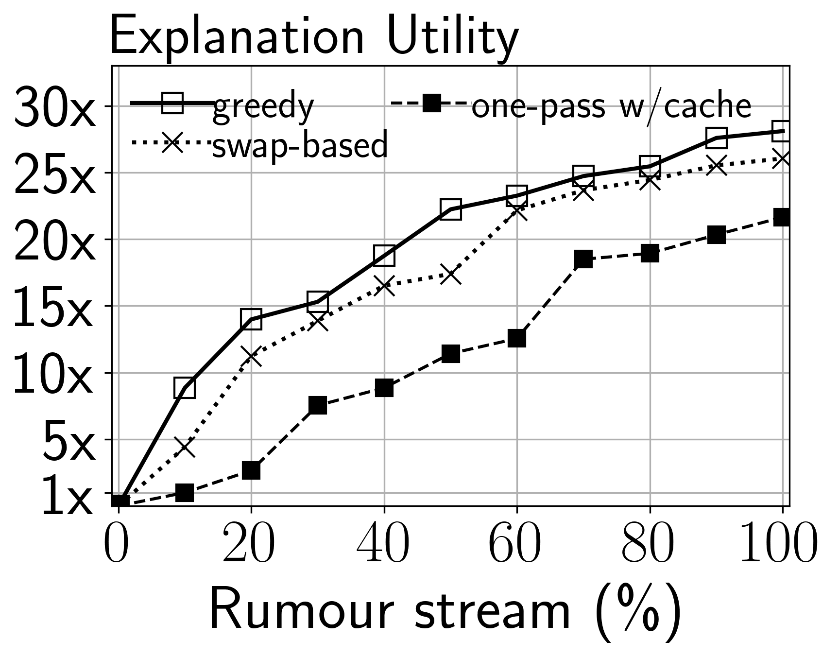
We observe that the utility increases greatly over time. At the beginning, the utility increases slowly, as there is not yet sufficient information for the derivation of an explanation. However, the utility improves quickly and converges. For example, in the Snopes dataset, with the greedy selection, the utility increases with only 50% of rumours. This indicates that the approach can incorporate the information of the multi-modal social graph quickly and provide useful explanations. Interestingly, different datasets exhibits different scales of utility improvement. For example, the greedy selection can reach more than improvement with 50% on the Anomaly dataset. This can be attributed to the fact that larger social graphs cover more features and structural information, which can be exploited to derive explanations.
8.5 Correctness of Rumour Embedding
Now, we assess whether the embeddings of structurally-similar subgraphs are indeed close in the embedding space. Our hypothesis is that there is a correlation between the cosine similarity of our graph embeddings and traditional graph similarity measures, including MCS, graphsim, and GED. To enable the use of MCS, for each dataset, we randomly extract subgraphs of size 15 from the social graph. We then select 10K pairs of subgraphs randomly and compute the size of their maximum common subgraphs. In the comparison with graphsim, we follow a similar procedure, but select pairs of subgraphs of the same size. As for GED, we generate a pair of subgraphs with edit distance by first constructing a two-hop ego graph from a randomly-selected node in the data graph. We then remove edges randomly, so that the subgraph is still connected, to obtain a subgraph . For each pair of subgraphs in every setting, we also measure their embedding similarity.
| Snopes | Anomaly | COVID | |
|---|---|---|---|
| MCS | 0.79 | 0.81 | 0.80 |
| graphsim | 0.89 | 0.88 | 0.87 |
| GED | -0.95 | -0.93 | -0.96 |

Table 2 confirms our hypothesis: There is a strong correlation between our embedding similarity and the graph similarity measures, reflected by Pearson’s correlation coefficients. GED has the strongest correlation (a negative correlation, as GED is a distance measure), since, similar to our embedding, it incorporates the whole structure of subgraphs, not only their common part. Fig. 12 further shows the average embedding similarity for each GED value. Here, values are normalised to by dividing by the maximum embedding similarity and the maximum GED value. Over all datasets, the GED and the embedding similarity behave consistently.
8.6 Efficiency of Rumour Embedding
Embedding time. We evaluate the efficiency of our embedding method in building the model for the whole social graph (training) as well as indexing a new subgraph (testing). To this end, we extract random subgraphs of the datasets with the same number of nodes, varying from to . Then, we measure the training time for each graph and report the average at each graph size.
As seen in Fig. 14, larger graph sizes increase the embedding time. Yet, compared to generic graph embedding methods, runtimes are competitive [59]. In particular, the time to embed a new rumour is small ( for all cases), as required in streaming settings.


Similarity computation. When selecting relevant rumours for explanation, similarity computation is an important operation. In this experiment, we evaluate our similarity computation method based on embeddings against existing baseline measures, including graphsim, MCS, and GED. For each dataset, we measure the similarity computation time between all pairs of identified rumours and report the average time.
According to Fig. 14, our embedding-based method is very fast for graph similarity computation, taking only 1ms or less. Moreover, our method is 4-5 orders of magnitude faster than MCS and graphsim, which require the computation of connected components .
Indexing performance. Our embedding method can be seen as a graph indexing technique. Hence, we also compare it against graph indices, such as CTIndex or GGSX in terms of time required to create an index/vector for a subgraph. For our approach, this is the time required to construct an embedding after we already trained the model. In this experiment, we set the subgraph size to 32.
| Snopes | Anomaly | COVID | |
|---|---|---|---|
| CTIndex | 79ms1kB | 87ms1kB | 1326ms1kB |
| GGSX | 131ms14.01kB | 528ms232kB | 928ms814kB |
| Sub2vec | 1045ms356kB | 1021ms363kB | 1028ms335kB |
| Our | 20ms1kB | 22ms1kB | 23ms1kB |

Table 3 shows the difference in the efficiency of structure-based approaches and our embedding-based index. CTIndex requires at least 79ms to create an index and on large datasets like COVID, it would take 1.326s. GGSX performs better than CTIndex for larger datasets like COVID, but require 131ms for small datasets like Snopes. Sub2vec, a subgraph embedding technique, requires around 1s to generate the embedding for a subgraph. Our method is even faster, around one order of magnitude, and constructs an index in around 20ms. Note that we evaluate the indexing in isolation, without any performance improvements.
Turning to space requirements, we fixed the embedding size for both CTIndex and our approach, with a similar index size for a fair comparison. As such, CTIndex and our index both require 1kB space. The index size of GGSX, in turn, depends on the social graph and ranges from 14.01kB to 814kB. Sub2vec also uses a fixed space because the dimensions of the embeddings are often fixed regardless of the subgraph size. We conclude that our index has comparable size, but can be constructed much quicker.
8.7 Qualitative Analysis
To assess the quality of our rumour embedding model, Fig. 15 presents the t-SNE visualisation of the vectors of rumour and non-rumour subgraphs in the Anomaly dataset (other datasets exhibit similar results). Here, the rumours (red) are clustered and distant from non-rumour subgraphs (green). Moreover, there is no single cluster for all rumours, implying that we should incorporate not only relevancy but also diversity when deriving an explanation.
8.8 Adaptivity of Explanations
Finally, we consider the adaptivity of explanations in cases of concept drifts. To simulate such scenarios, we vary the data distribution by randomly reordering the appearances of detected rumours in terms of their similarity, such that the similarity distribution is normal or skewed. We also vary the input rate (the high rate is 5 to 10 times faster than the low rate). Then, we measure the F1-score as in § 8.2. The results are averaged over all datasets and 10 random runs for each configuration, with an explanation size of seven.
| Data | Input | Static | Dynamic | Dynamic embedding |
|---|---|---|---|---|
| dist. | rate | embedding | embedding | w/ drift detection |
| normal | low | +0.00% | +45.32% | +67.95% |
| high | +0.00% | +45.04% | +67.95% | |
| skewed | low | -23.25% | +33.98% | +61.79% |
| high | -23.25% | +22.95% | +61.79% |
Table 4 presents the results for three versions of our framework: static embedding, a baseline where the model is not updated; dynamic embedding, where the model is updated as explained in § 7.3 after a fixed amount of time; and dynamic embedding w/ drift detection, where the model is updated when a concept drift is detected as presented in § 7.3. We report the difference in the F1-score from the baseline. Dynamic embedding turns out to improve the performance in adverse conditions, while drift detection further improves the robustness to different input rates and data distributions.
9 Conclusions
With the detection of rumours on social media becoming an increasingly important task, in this paper, we presented an approach to help users understand why certain entities are classified as a rumour. To this end, we followed the paradigm of example-based explanations of rumours for a graph-based model. That is, given a rumour graph, our approach extracts the most similar subgraphs that represent past rumours, while ensuring a certain level of diversity in the result. To achieve efficient construction of explanations, we proposed a novel technique for graph representation learning that incorporates both, features and modalities of nodes and edges. Further optimizations include indexing and caching schemes, as well as means to adapt to concept drift. Our experiments with diverse datasets highlight the efficiency and effectiveness of our approach. Especially, our approach yields explanations of much higher accumulated utility, up to a factor of , than baseline techniques. This implies that users would receive more information when investigating rumours with our explanation framework.
One limitation of our work is that explanations are based on real samples, so that some users might find it difficult to generalise from them. One possible improvement is include synthetic samples as additional explanation for users to compare, which however might overwhelm user cognitive load. In future work, we plan to use our explanations for downstream applications, such as group attack detection. Also, we intend to investigate the consensus computing of user feedback on explanation utility [58] and the integration of pseudo feedback mechanisms [56, 57].
References
- [1] S. Vosoughi, D. Roy, S. Aral, The spread of true and false news online, Science 359 (6380) (2018) 1146–1151.
- [2] N. T. Tam, M. Weidlich, B. Zheng, H. Yin, N. Q. V. Hung, B. Stantic, From anomaly detection to rumour detection using data streams of social platforms, PVLDB 12 (9) (2019) 1016–1029.
- [3] T. Cai, J. Li, A. Mian, R.-H. Li, T. Sellis, J. X. Yu, Target-aware holistic influence maximization in spatial social networks, TKDE 34 (4) (2022) 1993–2007.
- [4] R. E. Prasojo, M. Kacimi, W. Nutt, News: News event walker and summarizer, in: SIGMOD, 2019, pp. 1973–1976.
- [5] L. V. Lakshmanan, M. Simpson, S. Thirumuruganathan, Combating fake news: a data management and mining perspective, PVLDB 12 (12) (2019) 1990–1993.
- [6] J. C. Reis, A. Correia, F. Murai, A. Veloso, F. Benevenuto, Explainable machine learning for fake news detection, in: WebSci, 2019, pp. 17–26.
- [7] F. Yang, S. K. Pentyala, S. Mohseni, M. Du, H. Yuan, R. Linder, E. D. Ragan, S. Ji, X. Hu, Xfake: Explainable fake news detector with visualizations, in: WWW, 2019, pp. 3600–3604.
- [8] K. Shu, L. Cui, S. Wang, D. Lee, H. Liu, defend: Explainable fake news detection, in: KDD, 2019, pp. 395–405.
- [9] K. H. Tran, A. Ghazimatin, R. Saha Roy, Counterfactual explanations for neural recommenders, in: SIGIR, 2021, pp. 1627–1631.
- [10] Y. Mathov, E. Levy, Z. Katzir, A. Shabtai, Y. Elovici, Not all datasets are born equal: On heterogeneous tabular data and adversarial examples, Knowledge-Based Systems 242 (2022) 108377.
- [11] R. K. Mothilal, A. Sharma, C. Tan, Explaining machine learning classifiers through diverse counterfactual explanations, in: FAccT, 2020, pp. 607–617.
- [12] S. Barocas, A. D. Selbst, M. Raghavan, The hidden assumptions behind counterfactual explanations and principal reasons, in: FAccT, 2020, pp. 80–89.
- [13] W. Wang, J. Lu, T. Tong, Z. Liu, Debiased learning and forecasting of first derivative, Knowledge-Based Systems 236 (2022) 107781.
- [14] P. Mazumder, P. Singh, Protected attribute guided representation learning for bias mitigation in limited data, Knowledge-Based Systems 244 (2022) 108449.
- [15] C. T. Duong, T. D. Hoang, H. Yin, M. Weidlich, Q. V. H. Nguyen, K. Aberer, Efficient streaming subgraph isomorphism with graph neural networks, PVLDB 14 (5) (2021) 730–742.
- [16] S. Kumar, R. Asthana, S. Upadhyay, N. Upreti, M. Akbar, Fake news detection using deep learning models: A novel approach, ETT 31 (2) (2020) e3767.
- [17] X. Zhou, R. Zafarani, A survey of fake news: Fundamental theories, detection methods, and opportunities, CSUR 53 (5) (2020) 1–40.
- [18] Q. Huang, C. Zhou, J. Wu, M. Wang, B. Wang, Deep structure learning for rumor detection on twitter, in: IJCNN, 2019, pp. 1–8.
- [19] Q. Huang, J. Yu, J. Wu, B. Wang, Heterogeneous graph attention networks for early detection of rumors on twitter, in: IJCNN, 2020, pp. 1–8.
- [20] Q. Huang, C. Zhou, J. Wu, L. Liu, B. Wang, Deep spatial–temporal structure learning for rumor detection on twitter, Neural Computing and Applications (2020) 1–11.
- [21] N. T. Tam, M. Weidlich, D. C. Thang, H. Yin, N. Q. V. Hung, Retaining data from streams of social platforms with minimal regret, in: Proceedings of the Twenty-Sixth International Joint Conference on Artificial Intelligence, IJCAI-17, 2017, pp. 2850–2856.
- [22] N. Q. V. Hung, H. H. Viet, N. T. Tam, M. Weidlich, H. Yin, X. Zhou, Computing crowd consensus with partial agreement, IEEE Transactions on Knowledge and Data Engineering 30 (1) (2017) 1–14.
- [23] T. T. Nguyen, T. T. Huynh, H. Yin, V. Van Tong, D. Sakong, B. Zheng, Q. V. H. Nguyen, Entity alignment for knowledge graphs with multi-order convolutional networks, IEEE Transactions on Knowledge and Data Engineering (2020).
- [24] T. T. Nguyen, M. T. Pham, T. T. Nguyen, T. T. Huynh, Q. V. H. Nguyen, T. T. Quan, et al., Structural representation learning for network alignment with self-supervised anchor links, Expert Systems with Applications 165 (2021) 113857.
- [25] Z. Ying, D. Bourgeois, J. You, M. Zitnik, J. Leskovec, Gnnexplainer: Generating explanations for graph neural networks, NIPS 32 (2019).
- [26] X. Song, J. Li, Q. Lei, W. Zhao, Y. Chen, A. Mian, Bi-clkt: Bi-graph contrastive learning based knowledge tracing, Knowledge-Based Systems 241 (2022) 108274.
- [27] X. Song, J. Li, Y. Tang, T. Zhao, Y. Chen, Z. Guan, Jkt: A joint graph convolutional network based deep knowledge tracing, Information Sciences 580 (2021) 510–523.
- [28] G. Xue, M. Zhong, J. Li, J. Chen, C. Zhai, R. Kong, Dynamic network embedding survey, Neurocomputing 472 (2022) 212–223.
- [29] X. Zhang, F. T. Chan, S. Mahadevan, Explainable machine learning in image classification models: An uncertainty quantification perspective, Knowledge-Based Systems 243 (2022) 108418.
- [30] Y. Chang, Z. Ren, T. T. Nguyen, W. Nejdl, B. W. Schuller, Example-based explanations with adversarial attacks for respiratory sound analysis, in: Interspeech, 2021.
- [31] T. C. Phan, T. T. Nguyen, M. Weidlich, H. Yin, J. Jo, Q. V. H. Nguyen, exrumourlens: Auditable rumour detection with multi-view explanations, in: ICDE, 2022.
- [32] Y. Sun, J. Han, X. Yan, P. S. Yu, T. Wu, Pathsim: Meta path-based top-k similarity search in heterogeneous information networks, PVLDB 4 (11) (2011) 992–1003.
- [33] Y. Fang, Y. Yang, W. Zhang, X. Lin, X. Cao, Effective and efficient community search over large heterogeneous information networks, PVLDB 13 (6) (2020) 854–867.
- [34] M. Han, H. Kim, G. Gu, K. Park, W.-S. Han, Efficient subgraph matching: Harmonizing dynamic programming, adaptive matching order, and failing set together, in: SIGMOD, 2019, pp. 1429–1446.
- [35] S. Wang, T. Terano, Detecting rumor patterns in streaming social media, in: Big Data, 2015, pp. 2709–2715.
- [36] M. Dong, B. Zheng, N. Quoc Viet Hung, H. Su, G. Li, Multiple rumor source detection with graph convolutional networks, in: CIKM, 2019, pp. 569–578.
- [37] J. van der Waa, E. Nieuwburg, A. Cremers, M. Neerincx, Evaluating xai: A comparison of rule-based and example-based explanations, Artificial Intelligence 291 (2021) 103404.
- [38] H. Yu, D. Yuan, Subgraph search in large graphs with result diversification, in: SDM, 2014, pp. 1046–1054.
- [39] Y. Zhu, L. Qin, J. X. Yu, Y. Ke, X. Lin, High efficiency and quality: large graphs matching, VLDBJ 22 (3) (2013) 345–368.
- [40] B. Adhikari, Y. Zhang, N. Ramakrishnan, B. A. Prakash, Sub2vec: Feature learning for subgraphs, in: PAKDD, 2018, pp. 170–182.
- [41] T. Jin, Y. Yang, R. Yang, J. Shi, K. Huang, X. Xiao, Unconstrained submodular maximization with modular costs: Tight approximation and application to profit maximization, PVLDB 14 (10) (2021).
- [42] W. Hamilton, Z. Ying, J. Leskovec, Inductive representation learning on large graphs, in: NIPS, 2017, pp. 1024–1034.
- [43] R. Yang, J. Shi, X. Xiao, Y. Yang, J. Liu, S. S. Bhowmick, Scaling attributed network embedding to massive graphs, PVLDB 14 (1) (2020) 37–49.
- [44] A. Guttman, R-trees: A dynamic index structure for spatial searching, in: SIGMOD, 1984, pp. 47–57.
- [45] M. De Berg, O. Cheong, M. Van Kreveld, M. Overmars, Orthogonal range searching: Querying a database, Computational Geometry (2008) 95–120.
- [46] T. Stepišnik, D. Kocev, Oblique predictive clustering trees, Knowledge-Based Systems 227 (2021) 107228.
- [47] X. Zheng, P. Li, X. Hu, K. Yu, Semi-supervised classification on data streams with recurring concept drift and concept evolution, Knowledge-Based Systems 215 (2021) 106749.
- [48] K. Popat, S. Mukherjee, J. Strötgen, G. Weikum, Where the truth lies: Explaining the credibility of emerging claims on the web and social media, in: WWW Companion, 2017, pp. 1003–1012.
- [49] S. Montariol, M. Martinc, L. Pivovarova, Scalable and interpretable semantic change detection, in: NAACL-HLT, 2021, pp. 4642–4652.
- [50] Z. Wang, W. Dong, W. Zhang, C. W. Tan, Rumor source detection with multiple observations: Fundamental limits and algorithms, SIGMETRICS 42 (1) (2014) 1–13.
- [51] V. Bonnici, A. Ferro, R. Giugno, A. Pulvirenti, D. Shasha, Enhancing graph database indexing by suffix tree structure, in: IAPR-PRIB, Springer, 2010, pp. 195–203.
- [52] K. Klein, N. Kriege, P. Mutzel, Ct-index: Fingerprint-based graph indexing combining cycles and trees, in: ICDE, 2011, pp. 1115–1126.
- [53] P. Xuan, H. Cui, H. Zhang, T. Zhang, L. Wang, T. Nakaguchi, H. B. Duh, Dynamic graph convolutional autoencoder with node-attribute-wise attention for kidney and tumor segmentation from ct volumes, Knowledge-Based Systems 236 (2022) 107360.
- [54] Z. Zhang, Multi-layer attention aggregation in deep neural network, in: ITAIC, 2019, pp. 134–138.
- [55] B. Wang, X. Hu, P. Li, S. Y. Philip, Cognitive structure learning model for hierarchical multi-label text classification, Knowledge-Based Systems 218 (2021) 106876.
- [56] W. Gan, J. C.-W. Lin, P. Fournier-Viger, H.-C. Chao, H. Fujita, Extracting non-redundant correlated purchase behaviors by utility measure, Knowledge-Based Systems 143 (2018) 30–41.
- [57] M. Zhao, J. Liu, Z. Zhang, J. Fan, A scalable sub-graph regularization for efficient content based image retrieval with long-term relevance feedback enhancement, Knowledge-based systems 212 (2021) 106505.
- [58] S. F. Nimmy, O. K. Hussain, R. K. Chakrabortty, F. K. Hussain, M. Saberi, Explainability in supply chain operational risk management: A systematic literature review, Knowledge-Based Systems 235 (2022) 107587.
- [59] R. Zhu, K. Zhao, H. Yang, W. Lin, C. Zhou, B. Ai, Y. Li, J. Zhou, Aligraph: A comprehensive graph neural network platform, PVLDB 12 (12) (2019) 2094–2105.