ML-based Modeling to Predict I/O Performance on Different Storage Sub-systems
Abstract
Parallel applications can spend a significant amount of time performing I/O on large-scale supercomputers. Fast near-compute storage accelerators called burst buffers can reduce the time a processor spends performing I/O and mitigate I/O bottlenecks. However, determining if a given application could be accelerated using burst buffers is not straightforward even for storage experts. The relationship between an application’s I/O characteristics (such as I/O volume, processes involved, etc.) and the best storage sub-system for it can be complicated. As a result, adapting parallel applications to use burst buffers efficiently is a trial-and-error process. In this work, we present a Python-based tool called PrismIO that enables programmatic analysis of I/O traces. Using PrismIO, we identify bottlenecks on burst buffers and parallel file systems and explain why certain I/O patterns perform poorly. Further, we use machine learning to model the relationship between I/O characteristics and burst buffer selections. We run IOR (an I/O benchmark) with various I/O characteristics on different storage systems and collect performance data. We use the data as the input for training the model. Our model can predict if a file of an application should be placed on BBs for unseen IOR scenarios with an accuracy of 94.47% and for four real applications with an accuracy of 95.86%.
Index Terms:
I/O performance, trace analysis tool, benchmarking, machine learning, modelingI Introduction
Some high performance computing (HPC) applications can suffer from I/O performance bottlenecks due to slower advances in storage hardware technology as compared to compute hardware [1]. Such I/O bottlenecks can have a significant impact on the overall application performance [2], thus people create new I/O subsystems to improve applications performance. Recently, one type of I/O subsystem that is gaining more attention is the burst buffer.
Burst buffers (BBs) are fast intermediate storage layers positioned between compute nodes and hard disk storage [3]. Besides doing I/O all the time on the parallel file system (PFS), applications can let I/O go through BB and write back to the parallel file system at the end of the job. Therefore, BBs are suitable for applications with frequent checkpointing and restart[4]. Studies also show that BBs can accelerate I/O for a variety of HPC applications [4, 5, 6, 7, 8]. For instance, Bhimji et al. [7] demonstrate several types of applications including scientific simulation, data analysis, etc. can achieve better performance on BBs.
Although burst buffers have the potential to improve I/O performance, determining if an application could be accelerated by putting files on burst buffers is a complex task. First, the underlying relationship between an application’s I/O characteristics and its performance on I/O subsystems can be considerably complicated. In this paper, we use I/O characteristics to refer to things that decide the I/O behavior of an application, such as I/O volume, I/O library used, etc. For instance, the amount of data transferred per read or write, which we refer to as transfer size in the rest of the paper, can impact the I/O subsystem choices. For a very simple example, we did several IOR [9] runs with all configurations the same except different transfer sizes when writing files on Lassen GPFS (the regular parallel file system on Lassen) and BBs. We find that with a smaller transfer size it performs better on BB, while with a larger transfer size it performs better on GPFS (Figure 1). Varying other configurations of IOR can also lead to significant performance differences. We did a suite of IOR runs with various configurations on both systems, and the most extreme one among them runs 10x faster on GPFS than on BB. In later sections we present case studies on them and explain such cases through detailed analysis.

Second, even though we can manually figure out whether to direct the I/O of an application to BBs by doing experiments, it is a trial-and-error process. There is no work making the I/O subsystem selection an efficient workflow for arbitrary applications. Moreover, even a single application can read from or write to multiple files with different I/O characteristics. I/O to some files can have characteristics that perform better on GPFS, while I/O to other files can have characteristics that perform better on BBs. Figuring out the placement of each file manually for large-scale HPC applications is unrealistic.
Lastly, doing detailed analyses is challenging as well. Understanding why certain I/O characteristics perform well or poorly on certain I/O subsystems through detailed analyses is important. Detailed analyses can inspire insights for optimizations. They also help us validate our decision of choosing BBs or not. However, doing so is not trivial. Users have to make considerable efforts to write their own codes for the analysis, as existing tools are not efficient enough for detailed analysis. They lack of interfaces that enable users to customize their analysis.
We address the challenges by providing a methodology to conduct detailed analysis and model the selection of storage sub-systems using machine learning for HPC applications. We first present our performance analysis tool (PrismIO) and several case studies we did with it. We identify the bottlenecks of certain systems and explain why. PrismIO provides a data structure and APIs that enable users to customize their analysis. It also provides API to extract the I/O characteristics of an application. Next, we model the relationship between I/O characteristics and burst buffer selections using machine learning. We run IOR with various I/O characteristics on several I/O subsystem installations and collect performance data. With the data, we train models that select the best I/O subsystem for files of an application based on its I/O characteristics. Finally, we present a workflow that efficiently extracts I/O characteristics of applications, executes the model, and gives the file placement plan.
The main contributions of this work are:
-
•
We build a tool called PrismIO that enables detailed analysis of I/O traces. We identify and reason about different patterns/bottlenecks of I/O subsystems.
-
•
We conduct detailed experiments to study the relationship between I/O characteristics and the best storage sub-system choices. The resulting dataset can be used to model this relationship.
-
•
We train a machine learning model that approximates this relationship on Lassen. The model predicts whether to place files on BBs or GPFS based on I/O patterns with 94.47% accuracy.
-
•
To make it easy to train ML models, we add API functions in PrismIO that extract I/O characteristics and integrate the modeling workflow into PrismIO.
II Background & related work
In this section, we provide relevant literature needed to understand our work. We introduce BB, its architecture, and how it benefits I/O performance based on previous research. We also provide previous works that study how to better use BB and the limitations they found. Besides, we introduce performance analysis tools for I/O and their limitations.
II-A Burst buffers
Burst Buffers (BBs) are fast intermediate storage layers between compute nodes and storage nodes [3]. The traditional HPC I/O architecture consists of on-node memory, I/O nodes for handling I/O requests, and a disk-based parallel file system [10]. But this architecture is not enough to fill the gap between computational performance and I/O performance [7]. Therefore, BB is a natural solution to be introduced between these layers. BBs are implemented on several state-of-the-art HPC clusters such as Lassen, Summit, and Cori.
Burst buffers can be implemented in various ways. In terms of hardware, BBs are mostly made with SSDs. For example, Lassen at LLNL uses 1.6 TB Samsung PM1725a NVMe SSDs [11]. In terms of architecture, there are two major types: node-local and shared BBs [12]. Lassen and Summit adapt node-local BBs. In this case, a BB is directly connected to a compute node. All BBs are independent, which means they don’t share the same namespace. For the shared BBs (as used in Cori), BB nodes are separated from compute nodes and can be accessed by multiple compute nodes through interconnected networks [13]. In this case, compute nodes perform I/O on the global BB file system with a shared namespace. In this paper, we focus on node-local BBs.
Research has demonstrated the benefit BB brings to I/O performance [2]. For example, Bhimji et al. analyze the performance of a variety of HPC applications on Cori burst buffers, including scientific simulations, visualization, image reconstruction, and data analysis [7]. They demonstrate that burst buffers can accelerate the I/O of these applications and outperform regular Parallel File Systems (PFS). Pottier et al. [14] also demonstrate that node-local burst buffer significantly decreases the runtime and increases the bandwidth of an application called SWarp. From the research mentioned above [2, 14, 7], it is evident that BB has the potential to improve the I/O performance of certain HPC applications.
Although these papers demonstrate BB is promising in improving I/O performance, most of them raise the same concern: The performance is sensitive to application I/O patterns [7, 8, 14]. Pottier et al. demonstrated different workflows may not get the same benefit from BBs [14]. Some of them have decreased performance compared with the performance on regular file systems. For instance, they indicated that the shared burst buffer can perform worse than the regular PFS and is sensitive to the amount of data transferred per read/write operation. However, their work is only based on a single application called SWarp so it might not be general enough to cover common I/O patterns of HPC application. Existing research on this issue has not given a general solution to the problem due to insufficient experiments and modeling to cover different I/O patterns. Besides, the metric they use is the total runtime, which may not be a good I/O metric as it can be significantly affected by work other than I/O like computation. To summarize, the underlying relationship between an application’s I/O characteristics and the storage subsystem choice is still unclear.
II-B I/O performance analysis tools
There exist I/O performance analysis tools that can assist in studying such relationships. Two popular I/O performance analysis tools are PyDarshan [15, 16] and Recorder-viz [17]. Both of them trace application runs and capture basic performance information such as time and I/O volume of an operation. They provide visualization scripts upon their traces. With them users can derive aggregated I/O metrics such as I/O bandwidth, file sizes, etc. These tools can be helpful to start with the I/O subsystems selection research question, however, they are not efficient enough for detailed analysis due to the lack of interfaces that enable users to customize their analysis. Users have to make significant efforts to write their own codes to achieve deeper discoveries. Besides these two tracing tools, there is an automated analysis project called Tokio [18, 19], short for total knowledge of I/O. The project collects the I/O activities of all applications running on NERSC Cori for a time period and then provides a clear view of the system behavior. It does a great job in holistic I/O performance analyses such as detecting I/O contention and unhealthy storage devices at the system level. However, there is no application-level analysis so it does not map I/O characteristics to I/O subsystem selections.
III Data collection
To aid users in the appropriate selection of I/O subsystems to place files in their application, we conduct detailed analyses. We also leverage machine learning to model the relationship between I/O characteristics and the best I/O subsystems. Both of them require good supporting data. Therefore, the cornerstone of our work is to carefully design an experiment to build up a large and unbiased dataset. In this subsection, we introduce our experimental setup and data collection in detail. We go through machines, environments, benchmark configurations, and how we process the data.
III-A HPC machine and storage system
We conduct our experiment on Lassen. Lassen is a cluster at LLNL using IBM Power9 CPUs with 23 petaflops peak performance. It uses IBM’s Spectrum Scale parallel file systems, formerly known as GPFS. GPFS is one of the most common implementations of parallel file systems (PFS). It is used by many of the world’s supercomputers [20]. In terms of BB, Lassen uses node-local BBs implemented with Samsung NVMe PCIe SSDs.
III-B The IOR benchmark and its configuration
The benchmark we use is IOR [9]. We choose IOR because it is configurable enough to emulate various HPC workflows. It is proved to be an effective replacement for full-application I/O benchmarks [21] [22]. In our experiment, we select representative I/O characteristics that are common in real applications and configure IOR with them. For instance, we include collective MPI-IO because it’s a common characteristic in checkpoint/restart applications. We use IOR to emulate the I/O characteristics of real applications by covering all possible combinations of the selected I/O characteristics. We further separate I/O into six types, RAR, RAW, WAR, WAW, RO, and WO, to better map IOR runs with different types of applications (RAR for read after read, RAW for read after write, RO for read only, etc.). For instance, RAR and RO are common in ML applications between epochs. We again cover all feasible combinations of these read/write types and I/O characteristics.
We do the following to take variabilities into account. We repeat each run five times at different times and days to minimize the impact of temporal system variability. Since our whole experiment contains around 35,000 runs, we avoid adding abnormal burdens to the system and reflect system performance as normal as possible. We run them sequentially so at one time there is only one IOR run. We collect all I/O metrics from IOR standard output, including total I/O time, read/write time, bandwidth, etc, and take the mean of five iterations. Each IOR run produces a sample of the dataset.
III-C Data processing
The data we use is derived from IOR runs with different configurations on BB and GPFS, where each IOR run is a sample in the dataset. The independent variables are all I/O features we included in the experiment. Descriptions of them are presented in Table I. We first process them to make them suitable for common ML models. Most ML models cannot directly handle string-formatted categorical columns. Also, if a column is nominal instead of ordinal, simply converting it into integers ranging from 0 to the number of categories may result in erroneous inference. One popular solution is using one-hot vector encoding. It works by creating as many columns as the number of categories for a categorical column in the data set. Each column represents a category. We set a column to 1 if the original value is the category represented by that column and 0 for all other columns. We encode all our categorical columns such as file system, API, etc., into one-hot vectors.
| Input I/O feature | Description |
|---|---|
| I/O interface | Categorical feature |
| Can be POSIX, MPI-IO, HDF5 | |
| collective | Enable collective MPI-IO |
| fsync | Perform fsync after POSIX file close |
| preallocate | Preallocate the entire file before writing |
| transfer size | The amount of data of a single read/write |
| unique dir | Each process does I/O in its own directory |
| read/write per | The number of read/write |
| open to close | from open to close of a file |
| use file view | Use an MPI datatype for setting the file |
| view to use individual file pointer | |
| fsync per write | perform fsync upon POSIX write close |
| I/O type | Categorical feature |
| can be RAR, RAW, WAR, WAW, etc. | |
| random access | whether the file is randomly accessed |
As our goal is to classify the best I/O subsystem to place a file, the dependent variable should be the I/O subsystem. Recall that we run every I/O feature combination on both GPFS and BBs. We obtain the true label by selecting the I/O subsystem that gives the best I/O bandwidth for each particular I/O feature combination, which will be either GPFS or BB. The exhaustive I/O feature combinations plus the true label makes our final dataset. The final dataset has 19 feature columns and 2967 rows.
IV PrismIO: An I/O performance analysis tool
We have created PrismIO, a Python library that builds on top of Pandas [23, 24], as a solution to better facilitate detailed analysis. It has two primary benefits. First, it enables users to do analysis on a Pandas dataframe instead of an unfamiliar trace format. Based on the dataframe structure, PrismIO provides APIs that assist users in efficiently doing detailed analyses. Second, it provides functions that extract the I/O characteristics of applications. It is the foundation for applying our model to other applications because I/O characteristics are the input to the model.
IV-A Data structure
PrismIO is primarily designed for analyzing Recorder traces. Recorder [17] is an I/O tracing tool. It captures function calls from common I/O-related libraries such as fwrite, MPI_file_write, etc. We choose Recorder over Darshan because trace enables more detailed analysis than profiles. Recorder has a couple of APIs to generate plots, but it’s hard for users to efficiently customize analysis. To address this, we implement PrismIO as a Python library that builds on top of Pandas dataframe to organize data and build APIs upon it. The primary class that holds data and provides APIs is called IOFrame. It reorganizes the trace into a Pandas dataframe. Each row is a record of a function call. Columns store information of function calls, including start time, end time, the rank that calls the function, etc. It also explicitly lists information that is non-trivial to retrieve from the complex trace structure such as read/write access offset of a file.
IV-B API functions for analyzing I/O performance
PrismIO provides several analytical APIs that report aggregated information from different aspects, such as I/O bandwidth, I/O time, etc. It also provides feature extraction APIs that extract important I/O characteristics users may be interested in. These APIs will be part of our prediction workflow that we will discuss in later sections as they extract features needed for the model. In addition, PrismIO provides visualization of the trace. The following is a portion of frequently used APIs. Due to the space limit, we do not discuss all APIs in detail. Readers can check our GitHub repo for details if interested.
io_bandwidth One common analysis for I/O performance is to check the I/O bandwidth of each rank on different files. This function groups the dataframe by file name and rank and then calculates the bandwidth by dividing summed I/O volume by summed I/O time in each group. It provides options for quick filtering. It is common that people only want to focus on certain ranks in parallel application analysis. We provide a “rank” option that takes a list of ranks and filters out ranks that are listed before the groupby and aggregation. We also provide a general filter option where users can specify a filter function. The following code and Figure 2 demonstrate an example of using io_bandwidth.

io_time io_time returns the time spent in I/O by each rank on different files. Similar to io_bandwidth, users can filter different things. Figure 3 demonstrates an example of using it to check how much time rank 0, 1, 2, 3 spent in metadata operations (open, close, sync, etc.) on each file.

shared_files Another common analysis about parallel I/O is to see how files are shared across ranks. shared_files reports for each file, how many ranks are sharing it and what those ranks are. Figure 4 demonstrates part of the result of shared_files of a run.
IV-C Feature extraction API
Feature extraction is a class of APIs that extract the I/O characteristics of an application. As introduced previously, one primary purpose of these APIs is to prepare inputs to the model. In the machine learning context, the inputs to a model are called features. As our model models whether to place files on BBs based on I/O characteristics of applications, I/O characteristics are the input features to our model. In the rest of the paper, when we discuss topics related to the model, we use I/O features to refer to I/O characteristics. Such features include I/O type (RAR, RAW, WAR, etc.), access pattern (random or sequential), file per process (FPP), I/O interface (POSIX, MPI-IO, etc.), etc. For an arbitrary application, users either need to read the source code or analyze the trace to get them. With the original trace, users may spend considerable time writing code to analyze it, while with PrismIO, users can get those features by function calls. We provide examples to demonstrate the simplicity of using them.

access_pattern access_pattern counts the number of different access patterns including consecutive, sequential, and random access. Figure 5 demonstrates the access_pattern output of an example trace.

readwrite_pattern readwrite_pattern identifies read/write patterns such as RAR, RAW, etc., and calculates the amount of data transferred with those patterns. Figure 6 demonstrates the output of readwrite_pattern of a sample trace.

IV-D Visualization API
timeline The most-used visualization API in our use case study is timeline. It plots the timeline of function calls on each rank. Each line covers the time interval of a function execution, from start to end. It provides filter options for users to select certain types of functions. Figure 7 demonstrates an example timeline plot of I/O functions for a sample trace.

V Case studies
In this section, we present interesting case studies to demonstrate our analysis with PrismIO. We present insights that have not been systematically studied via large-scale experiments.


V-A Extreme runs analysis
We use IOR runs that perform quite differently between PFS and BB from the experiment dataset introduced in Section IV as our use cases for analysis and call them extreme runs. Figure 9 plots the I/O bandwidth of IOR runs with 64 processes on 2 nodes on GPFS and BB on Lassen. Each point represents a run with a certain I/O feature combination. The x-axis is the I/O bandwidth on PFS and the y-axis is the I/O bandwidth on BB. The farther the point from the diagonal, the IOR run with that configuration performs more differently on PFS and BB.

We pick the highlighted runs in Figure 9 to conduct detailed analyses. The upper left one performs much better on BBs than on PFS. The lower middle one performs much better on PFS than on BB. We refer to them as “Good BB Bad PFS” and “Good PFS Bad BB” in later text. Since they perform very differently between systems, they may indicate bottlenecks of systems. We trace them with Recorder, and then do detailed analyses with PrismIO.
Lassen GPFS bottleneck analysis: We first present the analysis for the “Good BB Bad PFS” run on Lassen. The I/O bandwidth per process for that run on GPFS is 155.01 MB/s, whereas on BB it is 3236.24 MB/s. Such a significant gap indicates there must be performance issues on GPFS for this run. We first utilize PrismIO io_time API and find the run on GPFS spends 37.8% of the I/O time in metadata operations. We then use the PrismIO timeline API introduced in section III to visualize the I/O function traces (Figure 10). We immediately observe a significant load imbalance of open over nodes on GPFS: the 32 processes on one node run much slower than 32 processes on the other node, but this is not happening on BB. We have checked the source code of IOR and logically all processes do exactly the same thing, so it is likely an issue with the system. To further drill down, we check if it is because that particular node is problematic or if it is a system issue.


We run IOR with the same configuration but on more nodes. Figure 8 demonstrates the I/O timeline of IOR runs on 2, 4, 8, 16 nodes. We noticed there is one and only one node that performs much better than the other nodes, so we checked if it is the same one in these four runs. Unfortunately, we did not observe a common node. Therefore, we conclude that it’s a system problem of GPFS in balancing metadata operations like open. We checked with LC admins and confirmed the low-level reason is that GPFS does not have metadata or data servers. When writing a bunch of files to the same directory, one of the nodes becomes the metadata server for that directory and thus ranks on it are much faster than ranks on other nodes for metadata operations.
Lassen BB bottleneck analysis: Similar to the previous section, we dive deeper to analyze the bottlenecks of Lassen BBs based on the “Good GPFS Bad BB” run. The run is running on 2 nodes with 32 processes per node as well. Figure 11 (a) (b) demonstrates the timeline for I/O function calls of each rank in that run on GPFS and BB, respectively. This time we observe a significant load imbalance over ranks on BB. Some ranks perform much worse than others, and such ranks are spread across both nodes. Besides, faster ranks on BB actually perform better than on GPFS. Furthermore, we noticed those faster ranks have unexpectedly high bandwidths, which indicates they are probably taking advantage of the SSD hardware cache. As it is part of the BB architecture, in most real-world use cases, applications have to use it by default. It does not make sense to exclude it from I/O performance modeling and analysis. To confirm this hypothesis, we run these IOR runs with the same configurations but with direct I/O enabled, in which case all I/O traffic would skip any kind of cache and directly go to storage.
Figure 11 (c) demonstrates the I/O timeline of the same run on BB but with direct I/O enabled. All ranks now take the same long time on BBs. This confirms that the load imbalance over ranks on BBs is due to the SSD hardware cache. GPFS is a shared file system so its hardware cache is likely to be occupied by millions of other workloads, while the hardware cache of node-local BBs is not filled until the total amount of I/O exceeds the cache size. When the hardware cache is filled, ranks with I/O that cannot use the cache have to run much slower than ranks with I/O that can use the cache. Therefore, the empirical conclusion from some research that large I/O does not perform well on BB is not completely correct. A single large I/O can still perform better on BB than on GPFS if the BB hardware cache is not full. Users can still do large I/O on BB, as long as the total amount of I/O at a time does not overwhelm the hardware cache.
V-B Overall trends
From the previous case studies, we identified some values of features that can be more preferable to BB. We saw MPI-IO, POSIX, transfer size, etc. can affect the choice of BB. Moreover, later in the model section, we get feature importance from the model. We will observe transfer size and read/write patterns are important features for the prediction. To give a summary of such trends, for a certain feature, we fix its value, and look at all runs with that feature equal to that value. We count how many runs are better on BB and PFS. Figure 12 demonstrates the percentage of runs better on Lassen BB as the values of features change. As transfer size grows, the percentage of runs better on BB decreases. Similarly, the percentage of runs better on BB is higher when reading than writing. We can conclude that although overall BB brings better performance than GPFS, it prefers smaller transfer sizes and read operations.


VI ML model for selecting best I/O sub-systems
We apply machine learning to efficiently recommend which file should be placed on which system, which we refer to as “file placement” in the rest of the paper. We design and train an ML model that selects the best I/O subsystems for application file placements. Moreover, to efficiently apply the model to an application when users don’t know its I/O characteristics, we make the selection process into a workflow with assistance from PrismIO feature extraction. In this section, we discuss the design of our models and the workflow.
VI-A Model design
The key to answering whether to place files written by an application on burst buffers is to understand the relationship between the I/O characteristics of an application and it’s performance on different I/O subsystems. As defined previously, we use I/O features to refer to I/O characteristics that we use as inputs to our model. Since some parameters are continuous such as transfer size and number of read/write, we need a model to interpolate the relationship. And since the parameter space is large, heuristic-based methods may not work well and are difficult to be extended when adding new I/O features. Therefore, we decided to apply machine learning (ML) techniques to model such relationships. An application can have multiple files with very different I/O patterns. These files from the same application can usually be placed on different I/O subsystems. Therefore, our model focuses on individual files instead of the whole application. Ideally, it predicts the best I/O subsystem for each file and thus results in the best file placement plan globally for the application.
Since Lassen uses node-local BBs, the target is either using it or not. So it should be a binary classification problem. We evaluate several different classifiers and compare their test accuracies. We do 90-10 split on our dataset. We train the model with 90% of the data, and then use the rest 10%, which is unseen for the model, to get the test accuracy by comparing predictions with the true labels. To mitigate the variability from data split, we train and evaluate each classifier 10 times with random data split every time. We report the test accuracy of the classifiers we tried in the result section.
VI-B Workflow for identifying best performing I/O sub-system
We make the selection process efficient by developing a workflow. This is because even though we obtained the approximation of the relationship with the ML model, applying it to large-scale HPC applications with a large number of different files is non-trivial. When users don’t know the I/O features of an application, they cannot apply the model. To solve this problem, we combine the feature extraction functions of PrismIO with the model and make them into a workflow. Figure 13 highlights the workflow design and demonstrates how parts fit together in the workflow and their inputs/outputs. Given an application, the user should only need to run it once on any machine and trace it with Recorder. Then the workflow would take the Recorder trace, extract I/O features for each file, and feed them into the pre-trained model to predict the best file placement, namely which file should be placed on which system for all files.

We have made the workflow a function called predict in PrismIO. Users simply need to call it with the trace path. It groups the data by file names and calls feature extraction APIs on each of them. It loads the model and predicts whether to use BBs for each file. The I/O features and predictions are organized as a dataframe indexed by file name. Figure 14 demonstrates a part of the workflow output of a sample trace.

VII Results
In this section, we present a comprehensive evaluation of our ML models. First, we report test accuracy for all classifiers we have tried on IOR benchmarking data. Second, we evaluate our prediction workflow with four real applications. We report the accuracy of the workflow on real applications.
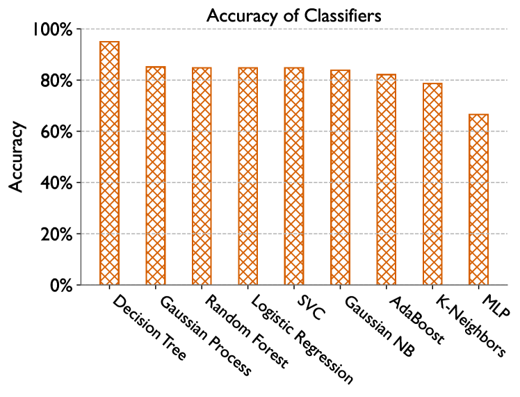
VII-A Comparing different ML models
We use the percentage of correct prediction to evaluate our classifiers. In other words, we compare the predictions with the ground truth and see what percentage it predicts the correct answer. We use accuracy to refer to this. For Lassen among the classifiers we tried, the Decision Tree classifier gives the highest test accuracy, which is 94.47% (Figure 15). Therefore, we decide to continue with the Decision Tree classifier.
The Decision Tree classifier has metrics for feature importance. Figure 16 demonstrates the importance of all features. Since our model predicts whether a combination of I/O features performs better on GPFS or BB, higher feature importance for model prediction implies the feature can be a key factor that distinguishes GPFS and BB. It may also imply underlying bottlenecks of a certain system. On the other hand, features with very low importance may be insignificant for prediction and accuracy. Therefore, features are selected after model selection by eliminating the least important features recursively until the accuracy significantly drops. After selecting the classifier and feature set, the chosen classifier is trained using the same data. This training is offline and the trained model can be loaded at runtime.

VII-B Model evaluation using production applications
In section V, we presented our test of the model on unseen IOR runs and got a 94.47% accuracy for Lassen. However, IOR is not a real application and we directly know the I/O features from the configurations of IOR runs. To further evaluate how our prediction workflow works on real applications, we test it with four unseen applications: LAMMPS, CM1, Paradis, and HACC-IO. LAMMPS is a molecular dynamics simulator, CM1 is an extreme climate simulator, Paradis is a dislocation dynamics simulator, and HACC-IO is the I/O proxy application of HACC, which is a cosmology simulator.
First, we run these applications on both Lassen GPFS and BBs and trace them with Recorder. Although we only need the trace on any one of the systems to make the prediction, we need both to get the ground truth. We run them with configurations from example use cases provided in the documentation or repository of these applications. Second, for each run, we apply our prediction workflow on either the GPFS trace or BB trace. As discussed in section V, it predicts which I/O subsystem to use for each file. Third, we get the ground truth of whether to use BBs for each file by comparing its I/O bandwidth on GPFS and BBs. We apply the PrismIO io_bandwidth API discussed in section III to get the I/O bandwidths of each file. Finally, we compare the predicted system with the ground truth to get accuracy.
We get 121 samples in our test data set. Since our model predicts whether to use BBs for a file based on its I/O features, each individual file produced by runs should be a sample. However, although these applications write a large number of files, many of them have exactly the same I/O features. For example, one LAMMPS run in our experiment has 386 different files, but most of them are dump files. LAMMPS does multiple dumps and it writes files in the same way for each dump. Such files will have exactly the same I/O features and the prediction for them will also be the same, meaning they cannot be used as different samples. Therefore, we create more application runs by varying their input configurations such as problem size, the number of processes, interfaces, etc. They will have more files with different I/O features and thus produce more samples. We group files with the same I/O features and treat them as a single sample. We use average bandwidth to figure out the ground truth for the group.

Figure 17 demonstrates the test accuracy. We achieve 95.86% accuracy on the whole test data set. For individual applications, we experimented with seven different HACC-IO cases and achieved 100% accuracy because it has quite simple I/O patterns. We experimented with two Paradis cases, three CM1 cases, and three LAMMPS cases to cover different I/O features. We achieved 96.67%, 96.55%, and 92% accuracy for Paradis, CM1, and LAMMPS, respectively.
VIII Conclusion
In this paper, we presented a prediction workflow that predicts whether to put files on BBs or not based on the I/O characteristics of an application. We did an experiment that covered a variety of I/O characteristics combinations using IOR. We trained and tested our model using the experiment data and it achieved 94.47% accuracy on unseen IOR data. Moreover, we developed feature extraction functions to apply our model to applications when we don’t know their I/O characteristics. we demonstrated use cases of the prediction workflow of runs of four real applications. It achieved 95.86% overall accuracy on those runs.
Besides the prediction workflow, we presented PrismIO, a Python-based library that enables programmatic analysis. It provides APIs for users to do detailed analyses efficiently. With the tool, we demonstrated two case studies where we utilized PrismIO to conduct detailed analyses. We explained the causes of two I/O performance issues on Lassen GPFS and BBs and made some empirical conclusions more complete. The case studies demonstrate the potential of PrismIO in making data analytics quick and convenient for the HPC user.
In the future, we plan to apply the same methodology to build prediction workflow for other platforms that have BBs such as Summit. Moreover, the current feature extraction APIs are not fast enough, therefore, we plan to improve their performance by designing better algorithms and creating APIs that extract multiple features at the same time. We believe that will make our prediction workflow more efficient for large application runs.
Acknowledgment
This work was performed under the auspices of the U.S. Department of Energy by Lawrence Livermore National Laboratory under Contract DE-AC52-07NA27344 (LLNL-CONF-858971). This material is based upon work supported by the U.S. Department of Energy, Office of Science, Office of Advanced Scientific Computing Research under the DOE Early Career Research Program.
References
- [1] A. Gainaru, G. Aupy, A. Benoit, F. Cappello, Y. Robert, and M. Snir, “Scheduling the i/o of hpc applications under congestion,” in 2015 IEEE International Parallel and Distributed Processing Symposium, 2015, pp. 1013–1022.
- [2] N. T. Hjelm, “libhio: Optimizing io on cray xc systems with datawarp,” 2017.
- [3] T. Wang, K. Mohror, A. Moody, K. Sato, and W. Yu, “An ephemeral burst-buffer file system for scientific applications,” in SC ’16: Proceedings of the International Conference for High Performance Computing, Networking, Storage and Analysis, 2016, pp. 807–818.
- [4] K. Sato, N. Maruyama, K. Mohror, A. Moody, T. Gamblin, B. R. de Supinski, and S. Matsuoka, “Design and modeling of a non-blocking checkpointing system,” in SC ’12: Proceedings of the International Conference on High Performance Computing, Networking, Storage and Analysis, 2012, pp. 1–10.
- [5] B. Nicolae, A. Moody, E. Gonsiorowski, K. Mohror, and F. Cappello, “Veloc: Towards high performance adaptive asynchronous checkpointing at large scale,” in 2019 IEEE International Parallel and Distributed Processing Symposium (IPDPS), 2019, pp. 911–920.
- [6] K. Sato, K. Mohror, A. Moody, T. Gamblin, B. R. d. Supinski, N. Maruyama, and S. Matsuoka, “A user-level infiniband-based file system and checkpoint strategy for burst buffers,” in 2014 14th IEEE/ACM International Symposium on Cluster, Cloud and Grid Computing, 2014, pp. 21–30.
- [7] W. Bhimji, D. Bard, M. Romanus, D. Paul, A. Ovsyannikov, B. Friesen, M. Bryson, J. Correa, G. K. Lockwood, V. Tsulaia, S. Byna, S. Farrell, D. Gursoy, C. Daley, V. Beckner, B. Van Straalen, D. Trebotich, C. Tull, G. H. Weber, N. J. Wright, K. Antypas, and n. Prabhat, “Accelerating science with the nersc burst buffer early user program,” 1 2016. [Online]. Available: https://www.osti.gov/biblio/1393591
- [8] A. Ovsyannikov, M. Romanus, B. Van Straalen, G. H. Weber, and D. Trebotich, “Scientific workflows at datawarp-speed: Accelerated data-intensive science using nersc’s burst buffer,” in 2016 1st Joint International Workshop on Parallel Data Storage and data Intensive Scalable Computing Systems (PDSW-DISCS), 2016, pp. 1–6.
- [9] “Ior.” [Online]. Available: https://ior.readthedocs.io/en/latest/index.html
- [10] Y.-F. Guo, Q. Li, G.-M. Liu, Y.-S. Cao, and L. Zhang, “A distributed shared parallel io system for hpc,” in Fifth International Conference on Information Technology: New Generations (itng 2008), 2008, pp. 229–234.
- [11] Using lc’s sierra systems. [Online]. Available: hpc.llnl.gov/documentation/tutorials/using-lc-s-sierra-systems
- [12] L. Cao, B. W. Settlemyer, and J. Bent, “To share or not to share: Comparing burst buffer architectures,” in Proceedings of the 25th High Performance Computing Symposium, ser. HPC ’17. San Diego, CA, USA: Society for Computer Simulation International, 2017.
- [13] B. R. Landsteiner, D. Henseler, D. Petesch, and N. J. Wright, “Architecture and design of cray datawarp,” 2016.
- [14] L. Pottier, R. F. da Silva, H. Casanova, and E. Deelman, “Modeling the performance of scientific workflow executions on hpc platforms with burst buffers,” in 2020 IEEE International Conference on Cluster Computing (CLUSTER), 2020, pp. 92–103.
- [15] Pydarshan documentation — pydarshan 3.3.1.0 documentation. [Online]. Available: https://www.mcs.anl.gov/research/projects/darshan/docs/pydarshan/index.html
- [16] P. Carns, K. Harms, W. Allcock, C. Bacon, S. Lang, R. Latham, and R. Ross, “Understanding and improving computational science storage access through continuous characterization,” ACM Trans. Storage, vol. 7, no. 3, oct 2011. [Online]. Available: https://doi.org/10.1145/2027066.2027068
- [17] C. Wang, J. Sun, M. Snir, K. Mohror, and E. Gonsiorowski, “Recorder 2.0: Efficient parallel i/o tracing and analysis,” in 2020 IEEE International Parallel and Distributed Processing Symposium Workshops (IPDPSW), 2020, pp. 1–8.
- [18] G. K. Lockwood, S. Snyder, S. Byna, P. Carns, and N. J. Wright, “Understanding data motion in the modern hpc data center,” in 2019 IEEE/ACM Fourth International Parallel Data Systems Workshop (PDSW), 2019, pp. 74–83.
- [19] T. Wang, S. Byna, G. K. Lockwood, S. Snyder, P. Carns, S. Kim, and N. J. Wright, “A zoom-in analysis of i/o logs to detect root causes of i/o performance bottlenecks,” in 2019 19th IEEE/ACM International Symposium on Cluster, Cloud and Grid Computing (CCGRID), 2019, pp. 102–111.
- [20] D. Quintero, J. Bolinches, J. Chaudhary, W. Davis, S. Duersch, C. H. Fachim, A. Socoliuc, and O. Weiser, “Ibm spectrum scale (formerly gpfs),” 2020.
- [21] H. Shan, K. Antypas, and J. Shalf, “Characterizing and predicting the i/o performance of hpc applications using a parameterized synthetic benchmark,” in SC ’08: Proceedings of the 2008 ACM/IEEE Conference on Supercomputing, 2008, pp. 1–12.
- [22] J. M. Kunkel, J. Bent, J. Lofstead, and G. S. Markomanolis, “Establishing the io-500 benchmark,” 2017.
- [23] W. McKinney, Python for Data Analysis: Data Wrangling with Pandas, NumPy, and IPython. O’Reilly Media, 2017.
- [24] ——, “Data structures for statistical computing in python,” in Proceedings of the 9th Python in Science Conference, S. van der Walt and J. Millman, Eds., 2010, pp. 51 – 56.