Mixture-of-Supernets: Improving Weight-Sharing Supernet Training with Architecture-Routed Mixture-of-Experts
Abstract
Weight-sharing supernets are crucial for performance estimation in cutting-edge neural architecture search (NAS) frameworks. Despite their ability to generate diverse subnetworks without retraining, the quality of these subnetworks is not guaranteed due to weight sharing. In NLP tasks like machine translation and pre-trained language modeling, there is a significant performance gap between supernet and training from scratch for the same model architecture, necessitating retraining post optimal architecture identification.
This study introduces a solution called mixture-of-supernets, a generalized supernet formulation leveraging mixture-of-experts (MoE) to enhance supernet model expressiveness with minimal training overhead. Unlike conventional supernets, this method employs an architecture-based routing mechanism, enabling indirect sharing of model weights among subnetworks. This customization of weights for specific architectures, learned through gradient descent, minimizes retraining time, significantly enhancing training efficiency in NLP. The proposed method attains state-of-the-art (SoTA) performance in NAS for fast machine translation models, exhibiting a superior latency-BLEU tradeoff compared to HAT, the SoTA NAS framework for machine translation. Furthermore, it excels in NAS for building memory-efficient task-agnostic BERT models, surpassing NAS-BERT and AutoDistil across various model sizes. The code can be found at: https://github.com/UBC-NLP/MoS.
Mixture-of-Supernets: Improving Weight-Sharing Supernet Training with Architecture-Routed Mixture-of-Experts
Ganesh Jawaharμ♡††thanks: Some of the work was completed while Ganesh was interning at Meta. Haichuan Yang∞ Yunyang Xiong∞ Zechun Liu∞ Dilin Wang∞ Fei Sun∞ Meng Li∞ Aasish Pappu∞ Barlas Oguz∞ Muhammad Abdul-Mageedμ♢ Laks V.S. Lakshmananμ Raghuraman Krishnamoorthi∞ Vikas Chandra∞ μUniversity of British Columbia ∞Meta ♢MBZUAI ♡Google DeepMind [email protected], {haichuan, yunyang, zechunliu, wdilin, feisun, aasish, barlaso}@meta.com [email protected], [email protected], [email protected], {raghuraman, vchandra}@meta.com
1 Introduction


| Supernet | Weight sharing | Capacity | Overall Time () | Average BLEU () |
|---|---|---|---|---|
| HAT (Wang et al., 2020a) | Strict | Single Set | 508 hours | 25.93 |
| Layer-wise MoS | Flexible | Multiple Set | 407 hours (20%) | 27.21 (4.9%) |
| Neuron-wise MoS | Flexible | Multiple Set | 394 hours (22%) | 27.25 (5.1%) |
Neural architecture search (NAS) automates the design of high-quality architectures for natural language processing (NLP) tasks while meeting specified efficiency constraints (Wang et al., 2020a; Xu et al., 2021, 2022a). NAS is commonly treated as a black-box optimization (Zoph et al., 2018; Pham et al., 2018), but obtaining the best accuracy requires repetitive training and evaluation, which is impractical for large datasets. To address this, weight sharing is applied via a supernet, where subnetworks represent different model architectures (Pham et al., 2018).
Recent studies demonstrate successful direct use of subnetworks for image classification with performance comparable to training from scratch (Cai et al., 2020; Yu et al., 2020). However, applying this supernet approach to NLP tasks is more challenging, revealing a significant performance gap when using subnetworks directly. This aligns with recent NAS works in NLP (Wang et al., 2020a; Xu et al., 2021), which address the gap by retraining or finetuning the identified architecture candidates. This situation introduces uncertainties about the optimality of selected architectures and requires repeated training for obtaining final accuracy on the Pareto front, i.e., the best models for different efficiency (e.g., model size or inference latency) budgets. This work aims to enhance the weight-sharing mechanism among subnetworks to minimize the observed performance gap in NLP tasks.
The weight-sharing supernet is trained by iteratively sampling architectures from the search space and training their specific weights from the supernet. Standard weight-sharing (Yu et al., 2020; Cai et al., 2020) involves directly extracting the first few output neurons to create a smaller subnetwork (see Figure 1 (a)), posing two challenges due to limited model capacity. First, the supernet imposes strict weight sharing among architectures, causing co-adaptation (Bender et al., 2018; Zhao et al., 2021) and gradient conflicts (Gong et al., 2021). For example, in standard weight-sharing, if a 5M-parameters model is a subnetwork of a 90M-parameters model, 5M weights are directly shared. However, the optimal shared weights for the 5M model may not be optimal for the 90M model, leading to significant gradient conflicts during optimization (Gong et al., 2021). Second, the supernet’s overall capacity is constrained by the parameters of a single deep neural network (DNN), i.e., the largest subnetwork in the search space. However, when dealing with a potentially vast number of subnetworks (e.g., billions), relying on a single set of weights to parameterize all of them could be insufficient (Zhao et al., 2021).
To address these challenges, we propose a Mixture-of-Supernets (MoS) framework. MoS enables architecture-specific weight extraction, allowing smaller architectures to avoid sharing some output neurons with larger ones. Additionally, it allocates large capacity without being constrained by the number of parameters in a single DNN. MoS includes two variants: layer-wise MoS, where architecture-specific weight matrices are constructed based on weighted combinations of expert weight matrices at the level of sets of neurons, and neuron-wise MoS, which operates at the level of individual neurons in each expert weight matrix. Our proposed NAS method proves effective in constructing efficient task-agnostic BERT models (Devlin et al., 2019) and machine translation (MT) models. For efficient BERT, our best supernet outperforms SuperShaper (Ganesan et al., 2021) by 0.85 GLUE points, surpasses NAS-BERT (Xu et al., 2021) and AutoDistil (Xu et al., 2022a) in various model sizes ( parameters). Compared to HAT (Wang et al., 2020a), our top supernet reduces the supernet vs. standalone model gap by 26.5%, provides a superior pareto front for latency-BLEU tradeoff ( to ms), and decreases the steps needed to close the gap by 39.8%. A summary in the Table 1 illustrates the time savings and BLEU improvements of MoS supernets for the WMT’14 En-De task.
We summarize our key contributions:
-
1.
We propose a formulation that generalizes weight-sharing methods, encompassing direct weight sharing (e.g., once-for-all network (Cai et al., 2020), BigNAS (Yu et al., 2020)) and flexible weight sharing (e.g., few-shot NAS (Zhao et al., 2021)). This formulation enhances the expressive power of the supernet.
-
2.
We apply the MoE concept to enhance model capability. The model’s weights are dynamically generated based on the activated subnetwork architecture. Post-training, the MoE can be converted into equivalent static models as our supernets solely depend on the fixed subnetwork architecture after training. (3)
-
3.
Our experiments show that our supernets achieve SoTA NAS results in building efficient task-agnostic BERT and MT models.
2 Supernet - Fundamentals
A supernet, utilizing weight sharing, parameterizes weights for millions of architectures, offering rapid performance predictions and significantly reducing NAS search costs. The training objective can be formalized as follows. Let denote the training data distribution. Let , denote the training sample and label respectively, i.e., . Let denote an architecture uniformly sampled from the search space . Let denote the subnetwork with architecture , and be parameterized by the supernet model weights . Then, the training objective of the supernet can be given by,
| (1) |
The mentioned formulation is termed single path one-shot (SPOS) optimization (Guo et al., 2020) for supernet training. Another popular technique is sandwich training (Yu et al., 2020), where the largest (), smallest (), and uniformly sampled architectures () from the search space are jointly optimized.
3 Mixture-of-Supernets
Existing supernets typically have limited model capacity to extract architecture-specific weights. For simplicity, assume the model function is a fully connected layer (output , omitting bias term for brevity), where , , and . and correspond to the number of input and output features respectively. Then, the weights () specific to architecture with output features are typically extracted by taking the first rows111We assume the number of input features remains constant. If it changes, only the initial columns of are extracted. (as shown in Figure 1 (a)) from the supernet weight . Assume one samples two architectures ( and ) from the search space with the number of output features and respectively. Then, the weights corresponding to the architecture with the smallest number of output features will be a subset of those of the other architecture, sharing the first output features exactly. This weight extraction technique enforces strict weight sharing between architectures, irrespective of their global architecture information (e.g., different features in other layers). For example, architectures and may have vastly different capacities (e.g., vs parameters). The smaller architecture (e.g., ) must share all weights with the larger one (e.g., ), and the supernet (modeled by ) cannot allocate weights specific to the smaller architecture. Another issue with is that the supernet’s overall capacity is constrained by the parameters in the largest subnetwork () in the search space. Yet, these supernet weights must parameterize numerous diverse subnetworks. This represents a fundamental limitation of the standard weight-sharing mechanism. Section 3.1 proposes a reformulation to overcome this limitation, implemented through two methods (Layer-wise MoS, Section 3.2, Neuron-wise MoS, Section 3.3), suitable for integration into Transformers (see Section 3.4).
3.1 Generalized Model Function
We can reformulate the function to a generalized form , which takes 2 inputs: the input data , and the activated architecture . includes the learnable parameters of . Then, the training objective of the proposed supernet becomes,
| (2) |
For the standard weight sharing mechanism mentioned above, and function just uses to perform the “trimming” operation on the weight matrix , and forwards the subnetwork. To further minimize objective equation 2, enhancing the capacity of the model function is a potential approach. However, conventional methods like adding hidden layers or neurons are impractical here since the final subnetwork architecture of mapping to cannot be altered. This work introduces the concept of Mixture-of-Experts (MoE) (Fedus et al., 2022) to enhance the capacity of . Specifically, we dynamically generate weights for a specific architecture by routing to certain weight matrices from a set of expert weights. We term this architecture-routed MoE-based supernet as Mixture-of-Supernets (MoS) and design two routing mechanisms for function . Due to lack of space, the detailed algorithm for supernet training and search is shown in A.2.
3.2 Layer-wise MoS
Assume there are (number of experts) unique weight matrices (, or expert weights), which are learnable parameters. For simplicity, we only use a single linear layer as the example. For an architecture with output features, we propose the layer-wise MoS that computes the weights specific to the architecture (i.e. ) by performing a weighted combination of expert weights, . Here, corresponds to the standard top rows extraction from the expert weights. The alignment vector () captures the alignment scores of the architecture with respect to each expert (weights matrix). We encode the architecture as a numeric vector (e.g., a list of the number of output features for different layers), and apply a learnable router (an MLP with softmax) to produce such scores, i.e. . Thus, the generalized model function for the linear layer (as shown in Figure 1 (b)) can be defined as (omitting bias for brevity):
| (3) |
The router governs the degree of weight sharing between two architectures through modulation of alignment scores (). For instance, if and is a subnetwork of architecture , the supernet can allocate weights specific to the smaller architecture by setting and . In this scenario, exclusively utilizes weights from , and uses weights from , enabling updates to and towards the loss from architectures and without conflicts. It’s worth noting that few-shot NAS (Zhao et al., 2021) is a special case of our framework when the router is rule-based. Moreover, functions as an MoE, enhancing expressive power and reducing the objective equation 2. Once supernet training is done, for a given architecture , the score can be generated offline. Expert weights collapse, reducing the number of parameters for architecture to . Layer-wise MoS results in a lower degree of weight sharing between differently sized architectures, as evidenced by a higher Jensen-Shannon distance between their alignment probability vectors compared to similarly sized architectures. Refer to A.1.1 for more details.
3.3 Neuron-wise MoS
Layer-wise MoS employs a standard MoE setup, where each expert is a linear layer/module. The router determines the combination of experts to use for forwarding the input based on . In this setup, the degree of freedom for weight generation is , and the parameter count grows by , with being the parameters in the standard supernet. Therefore, a sufficiently large is needed for flexibility in subnetwork weight generation, but it also introduces too many parameters into the supernet, making layer-wise MoS challenging to train. To address this, we opt for a smaller granularity of weights to represent each expert, using neurons in DNN as experts. In terms of the weight matrix, neuron-wise MoS represents an individual expert with one row, whereas layer-wise MoS uses an entire weight matrix. For neuron-wise MoS, the router output for each layer, and the sum of each row in is 1. Similar to layer-wise MoS, we use an MLP to produce the matrix and apply softmax on each row. We formulate the function for neuron-wise MoS as
| (4) |
where constructs a diagonal matrix by putting on the diagonal, and is the -th column of . is still an matrix as in layer-wise MoS. Compared to layer-wise MoS, neuron-wise MoS offers increased flexibility ( instead of only ) to manage the degree of weight sharing between different architectures, with the number of parameters remaining proportional to . Neuron-wise MoS provides finer control over weight sharing between subnetworks. Gradient conflict, computed using cosine similarity between the supernet and smallest subnet gradients following NASVIT (Gong et al., 2021), is lowest for neuron-wise MoS compared to layer-wise MoS and HAT, as shown by the highest cosine similarity (see A.1.2).
3.4 Adding to Transformer
MoS is adaptable to a single linear layer, multiple linear layers, and other parameterized layers (e.g., layer-norm). Given that the linear layer dominates the number of parameters, we adopt the approach used in most MoE work (Fedus et al., 2022). We apply MoS to the standard weight-sharing-based Transformer () by replacing the two linear layers in every feed-forward network block with .
4 Experiments - Efficient BERT
| Supernet | Training time (hours) | MNLI | CoLA | MRPC | SST2 | QNLI | QQP | RTE | Avg. GLUE () |
|---|---|---|---|---|---|---|---|---|---|
| Standalone | - | 82.61 | 59.03 | 86.54 | 91.52 | 89.47 | 90.68 | 71.53 | 81.63 |
| Supernet (Sandwich) | 37 | 82.34 | 57.58 | 86.54 | 91.74 | 88.67 | 90.39 | 73.26 | 81.50 (-0.13) |
| Layer-wise MoS (ours) | 43 (16%) | 82.40 | 57.62 | 87.26 | 92.08 | 89.57 | 90.68 | 77.08 | 82.38 (+0.75) |
| Neuron-wise MoS (ours) | 45 (21.6%) | 82.68 | 58.71 | 87.74 | 92.16 | 89.22 | 90.49 | 76.39 | 82.48 (+0.85) |
| Supernet | #Params | #Steps | CoLA | MRPC | SST2 | QNLI | QQP | RTE | Avg. GLUE |
|---|---|---|---|---|---|---|---|---|---|
| NAS-BERT | 5M | 125K | 19.8 | 79.6 | 87.3 | 84.9 | 85.8 | 66.7 | 70.7 |
| AutoDistil (proxy) | 6.88M | 0 | 24.8 | 78.5 | 85.9 | 86.4 | 89.1 | 64.3 | 71.5 |
| Neuron-wise MoS | 5M | 0 | 28.3 | 82.7 | 86.9 | 84.1 | 88.5 | 68.1 | 73.1 |
| NAS-BERT | 10M | 125K | 34.0 | 79.1 | 88.6 | 86.3 | 88.5 | 66.7 | 73.9 |
| Neuron-wise MoS | 10M | 0 | 34.7 | 81.0 | 88.1 | 85.1 | 89.1 | 66.7 | 74.1 |
| AutoDistil (proxy) | 26.1M | 0 | 48.3 | 88.3 | 90.1 | 90.0 | 90.6 | 69.4 | 79.5 |
| AutoDistil (agnostic) | 26.8M | 0 | 47.1 | 87.3 | 90.6 | 89.9 | 90.8 | 69.0 | 79.1 |
| Neuron-wise MoS | 26.8M | 0 | 52.7 | 88.0 | 90.0 | 87.7 | 89.9 | 78.1 | 81.1 |
| NAS-BERT | 30M | 125K | 48.7 | 84.6 | 90.5 | 88.4 | 90.2 | 71.8 | 79.0 |
| Neuron-wise MoS | 30M | 0 | 51.0 | 87.3 | 91.1 | 87.9 | 90.2 | 72.2 | 80.0 |
| AutoDistil (proxy) | 50.1M | 0 | 55.0 | 88.8 | 91.1 | 90.8 | 91.1 | 71.9 | 81.4 |
| Neuron-wise MoS | 50M | 0 | 55.0 | 88.0 | 91.9 | 89.0 | 90.6 | 75.4 | 81.6 |
4.1 Experiment Setup
We explore the application of our proposed supernet in constructing efficient task-agnostic BERT (Devlin et al., 2019) models, focusing on the BERT pretraining task. This involves pretraining a language model from scratch to learn task-agnostic text representations using a masked language modeling objective. The pretrained BERT model is then finetuned on various downstream NLP tasks. Emphasis is on building highly accurate yet small BERT models (e.g., parameters). Both BERT supernet and standalone models are pretrained from scratch on Wikipedia and Books Corpus (Zhu et al., 2015). Performance evaluation is conducted by finetuning on seven tasks from the GLUE benchmark (Wang et al., 2018), chosen by AutoDistil (Xu et al., 2022a). The architecture encoding, data preprocessing, pretraining settings, and finetuning settings are detailed in A.4.1. Baseline models include standalone and standard supernet models proposed in SuperShaper (Ganesan et al., 2021). Our proposed models are layer-wise and neuron-wise MoS. All supernets undergo sandwich training 222SuperShaper notes that SPOS performs poorly compared to sandwich training; hence, we do not study SPOS for building BERT models. The learning curve is shown in A.4.2.. Parameters and router’s hidden dimension are set to and , respectively, for MoS supernets.
4.2 Supernet vs. standalone gap
For investigating the supernet vs. standalone gap, the search space is derived from SuperShaper (Ganesan et al., 2021), encompassing BERT architectures differing only in hidden size at each layer (120, 240, 360, 480, 540, 600, 768) with fixed numbers of layers () and attention heads (). This search space includes around billion architectures. We examine the supernet vs. standalone model gap for the top model architecture from the pareto front of Supernet (Sandwich) (Ganesan et al., 2021). Table 2 illustrates the GLUE benchmark performance of standalone training for the architecture (x pretraining budget, equivalent to 2048 batch size * 125,000 steps) as well as architecture-specific weights from different supernets ( additional pretraining steps; i.e., only supernet pretraining). MoS (layer-wise or neuron-wise) bridges the gap between task-specific supernet and standalone performance for out of tasks, including MNLI, a widely used task for evaluating pretrained language models (Liu et al., 2019; Xu et al., 2022b). The average GLUE gap between the standalone model and standard supernet is points. Remarkably, with customization and expressivity properties, layer-wise and neuron-wise MoS significantly improve standalone training by and average GLUE points, respectively. 333Consistency of these results across different seeds is discussed in A.4.5. Table 2 demonstrates that MoS imposes a computational overhead of under 22% for BERT, resulting in a minimum of 0.8 average GLUE improvement compared to the standard supernet. This overhead may not be significant, as it represents a one-time investment that eliminates the need for additional training after the search process.
4.3 Comparison with SoTA NAS
The SoTA NAS frameworks for constructing a task-agnostic BERT model are NAS-BERT (Xu et al., 2021) and AutoDistil (Xu et al., 2022a).444AutoDistil (proxy) outperforms SoTA distillation approaches such as TinyBERT (Jiao et al., 2020) and MINILM (Wang et al., 2020b) by average GLUE points. Hence, we do not compare against these works. The NAS-BERT pipeline comprises: (1) supernet training (with a Transformer stack containing multi-head attention, feed-forward network [FFN], and convolutional layers at arbitrary positions), (2) search based on the distillation (task-agnostic) loss, and (3) pretraining the best architecture from scratch (x pretraining budget, equivalent to 2048 batch size * 125,000 steps). The third step needs to be repeated for every constraint change and hardware change, incurring substantial costs. The AutoDistil pipeline involves: (1) constructing search spaces and training supernets for each search space independently, (2a) agnostic-search mode: searching based on the self-attention distillation (task-agnostic) loss, (2b) proxy-search mode: searching based on the MNLI validation score, and (3) extracting architecture-specific weights from the supernet without additional training. The first step can be costly as pretraining supernets requires times training compute and memory, compared to training a single supernet. The proxy-search mode may favor AutoDistil unfairly, as it finetunes all architectures in its search space on MNLI and utilizes the MNLI score for ranking. For a fair comparison with SoTA, MNLI task is excluded from evaluation. 555Refer to A.4.4 for a comparison of neuron-wise MoS against baselines that don’t directly tune on the MNLI task. Neuron-wise MoS consistently outperforms baselines in terms of both average GLUE and MNLI task performance.
Our proposed NAS pipeline addresses challenges in NAS-BERT and AutoDistil. In comparison to SoTA NAS, our search space includes BERT architectures with uniform Transformer layers: hidden size ( to in increments of ), attention heads (6, 12), intermediate FFN hidden dimension ratio (2, 2.5, 3, 3.5, 4). This search space comprises architectures, similar to AutoDistil. The supernet is based on neuron-wise MoS, and the search uses perplexity (task-agnostic) to rank architectures. Unlike NAS-BERT, our final architecture weights are directly extracted from the supernet without additional pretraining. Unlike AutoDistil, our pipeline pretrains only one supernet, significantly reducing training compute and memory. We use only task-agnostic metrics for search, similar to AutoDistil’s agnostic setting. Table 3 compares neuron-wise MoS supernet with NAS-BERT and AutoDistil for various model sizes. NAS-BERT and AutoDistil performances are obtained from respective papers. On average GLUE, our pipeline improves over NAS-BERT for , , and model sizes, with no additional training (100% additional training compute savings, equivalent to 2048 batch size * 125,000 steps). On average GLUE, our pipeline: (i) surpasses AutoDistil-proxy for and model sizes with and fewer parameters respectively, and (ii) outperforms both AutoDistil-proxy and AutoDistil-agnostic for model size. Besides achieving SoTA results, our method significantly reduces the heavy workload of training multiple models in subnetwork retraining (NAS-BERT) or supernet training (AutoDistil).
5 Experiments - Efficient MT
| Dataset | WMT’14 En-De | WMT’14 En-Fr | WMT’19 En-De | |||
|---|---|---|---|---|---|---|
| Supernet | MAE () | Kendall () | MAE () | Kendall () | MAE () | Kendall () |
| HAT | 1.84 | 0.81 | 1.37 | 0.63 | 2.07 | 0.71 |
| Supernet (Sandwich) | 1.62 (12%) | 0.81 | 1.37 (0%) | 0.63 | 2.02 (2.4%) | 0.87 |
| Layer-wise MoS (ours) | 1.61 (12.5%) | 0.54 | 1.24 (9.5%) | 0.73 | 1.57 (24.2%) | 0.87 |
| Neuron-wise MoS (ours) | 1.13 (38.6%) | 0.71 | 1.2 (12.4%) | 0.85 | 1.48 (28.5%) | 0.81 |
5.1 Experiment setup
We discuss the application of proposed supernets for building efficient MT models following the setup by Hardware-aware Transformers (HAT (Wang et al., 2020a)), the SoTA NAS framework for MT models with good latency-BLEU tradeoffs. Focusing on WMT’14 En-De, WMT’14 En-Fr, and WMT’19 En-De benchmarks, we maintain consistent architecture encoding and training settings for supernet and standalone models (details in A.5.2). Baseline supernets include HAT and Supernet (Sandwich). Proposed supernets are Layer-wise MoS and Neuron-wise MoS, both using sandwich training, with and router’s hidden dimension set to 2 and 128, respectively. Refer to A.5.8 for the rationale behind choosing ‘’.
5.2 Supernet vs. standalone gap
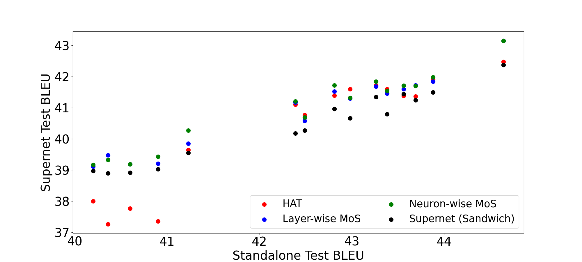
In HAT’s search space of encoder-decoder architectures, featuring flexible parameters like embedding size (512 or 640), decoder layers (1 to 6), self/cross attention heads (4 or 8), and number of top encoder layers for decoder attention (1 to 3), good supernets should exhibit minimal mean absolute error (MAE) and high rank correlation between supernet and standalone performance for a given architecture. Table 4 presents MAE and Kendall rank correlation for 15 random architectures, showcasing that sandwich training yields better MAE and rank quality compared to HAT. While our proposed supernets achieve comparable rank quality for WMT’14 En-Fr and WMT’19 En-De, and slightly underperform for WMT’14 En-De, they exhibit minimal MAE across all tasks. Particularly, neuron-wise MoS achieves substantial MAE improvements, suggesting lower additional training steps needed to make MAE negligible (as detailed in Section 5.4). Supernet and standalone performance plots reveal neuron-wise MoS excelling for almost all top-performing architectures (see A.5.3). The training overhead for MoS is generally negligible, e.g., for WMT’14 En-De, supernet training takes 248 hours, with neuron-wise MoS and layer-wise MoS requiring 14 and 18 additional hours, respectively (less than % overhead, see Section A.5.10 for details).
| Dataset | WMT’14 En-De | WMT’14 En-Fr | WMT’19 En-De | ||||||
|---|---|---|---|---|---|---|---|---|---|
| Supernet / Latency Constraint | 100 ms | 150 ms | 200 ms | 100 ms | 150 ms | 200 ms | 100 ms | 150 ms | 200 ms |
| HAT | 25.26 | 26.25 | 26.28 | 38.94 | 39.26 | 39.16 | 42.61 | 43.07 | 43.23 |
| Layer-wise MoS (ours) | 26.28 | 27.31 | 28.03 | 39.34 | 40.29 | 41.24 | 43.45 | 44.71 | 46.18 |
| Neuron-wise MoS (ours) | 26.37 | 27.59 | 27.79 | 39.55 | 40.02 | 41.04 | 43.77 | 44.66 | 46.21 |
5.3 Comparison with the SoTA NAS
The pareto front from the supernet is obtained using an evolutionary search algorithm that leverages the supernet for quickly identifying top-performing candidate architectures and a latency estimator for promptly discarding candidates with latencies surpassing a threshold. Settings for the evolutionary search algorithm and latency estimator are detailed in A.5.4. Three latency thresholds are explored: ms, ms, and ms. Table 5 illustrates the latency vs. supernet performance tradeoff for models in the pareto front from different supernets. Compared to HAT, the proposed supernets consistently achieve significantly higher BLEU for each latency threshold across all datasets, emphasizing the importance of architecture specialization and expressiveness of the supernet. See A.5.6 for the consistency of these trends across different seeds.
| Dataset | Additional training steps () | Additional training time (NVIDIA V100 hours) () | ||||
|---|---|---|---|---|---|---|
| Supernet | WMT’14 En-De | WMT’14 En-Fr | WMT’19 En-De | WMT’14 En-De | WMT’14 En-Fr | WMT’19 En-De |
| HAT | 33K | 33K | 26K | 63.9 | 60.1 | 52.3 |
| Laye. MoS | 16K (51.5%) | 30K (9%) | 20K (23%) | 35.5 (44.4%) | 66.5 (-10.6%) | 45.2 (13.5%) |
| Neur. MoS | 13K (60%) | 26K (21%) | 16K (38.4%) | 31.0 (51.4%) | 61.7 (-2.7%) | 39.5 (24.5%) |
5.4 Additional training to close the gap
The proposed supernets significantly minimize the gap between the supernet and standalone MAE (as discussed in Section 5.2), yet the gap remains non-negligible. Closing the gap for an architecture involves extracting architecture-specific weights from the supernet and conducting additional training until the standalone performance is reached (achieving a gap of ). An effective supernet should demand a minimal number of additional steps and time for the extracted architectures to close the gap. In the context of additional training, we evaluate the test BLEU for each architecture after every steps, stopping when the test BLEU matches or exceeds the test BLEU of the standalone model. Table 6 presents the average number of additional training steps required for all models on the pareto front from each supernet to close the gap. Compared to HAT, layer-wise MoS achieves an impressive reduction of % to % in training steps, while neuron-wise MoS delivers the most substantial reduction of % to %. For the WMT’14 En-Fr task, both MoS supernets require at least % more time than HAT to achieve SoTA BLEU across different constraints. These results underscore the importance of architecture specialization and supernet expressivity in significantly improving the training efficiency of subnets extracted from the supernet.
5.5 Comparison to AutoMoE
| Dataset | WMT’14 En-De | WMT’14 En-Fr | WMT’19 En-De |
|---|---|---|---|
| Supernet / Latency Constraint | 200 ms | 200 ms | 200 ms |
| HAT | 26.28 | 39.16 | 43.23 |
| AutoMoE | 26.06 | 38.98 | 43.13 |
| Layer-wise MoS (ours) | 28.03 | 41.24 | 46.18 |
| Neuron-wise MoS (ours) | 27.79 | 41.04 | 46.21 |
Although AutoMoE Jawahar et al. (2023) and MoS pursue distinct objectives (as discussed in Appendix A.3), we proceed to compare the supernet BLEU scores of HAT, AutoMoE, and MoS under a latency constraint of 200 ms on the NVIDIA V100 GPU across the three WMT benchmarks. Table 7 shows that MoS consistently outperforms AutoMoE and HAT across all datasets. Interestingly, AutoMoE falls behind HAT, suggesting a potential discrepancy between the performance of AutoMoE’s supernet and standalone models.
6 Related Work
In this section, we briefly review existing research on NAS in NLP. Evolved Transformer (ET) (So et al., 2019) is an initial work that explores NAS for efficient MT models. It employs evolutionary search and dynamically allocating training resources for promising candidates., HAT (Wang et al., 2020a) introduces a weight-sharing supernet as a performance estimator, amortizing the training cost for candidate MT evaluations in evolutionary search. NAS-BERT (Xu et al., 2021) partitions the BERT-Base model into blocks and trains a weight-sharing supernet to distill each block. NAS-BERT uses progressive shrinking during supernet training to prune less promising candidates, identifying top architectures for each efficiency constraint quickly. However, NAS-BERT requires pretraining the top architecture from scratch for every constraint change, incurring high costs. SuperShaper (Ganesan et al., 2021) pretrains a weight-sharing supernet for BERT using a masked language modeling objective with sandwich training. AutoDistil (Xu et al., 2022a) employs few-shot NAS (Zhao et al., 2021): constructing search spaces of non-overlapping BERT architectures and training a weight-sharing BERT supernet for each search space. The search is based on self-attention distillation loss with BERT-Base (task-agnostic search) and MNLI score (proxy search). AutoMoE (Jawahar et al., 2023) augments the search space of HAT with mixture-of-expert models to design efficient translation models. Refer to A.3 for the main differences between our framework and the AutoMoE framework.
In the computer vision community, K-shot NAS (Su et al., 2021) generates weights for each subnet as a convex combination of different supernet weights in a dictionary using a simplex code. While K-shot NAS shares similarities with layer-wise MoS, there are key distinctions. K-shot NAS trains the architecture code generator and supernet iteratively due to training difficulty, whereas layer-wise MoS trains all its components jointly. K-shot NAS has been applied specifically to convolutional architectures for image classification tasks. However, it introduces too many parameters with an increase in the number of supernets (), a concern alleviated by neuron-wise MoS due to its granular weight specialization. In our work, we focus on NLP tasks and relevant baselines, noting that supernets in NLP tend to lag significantly behind standalone models in terms of performance. Additionally, the authors of K-shot NAS have not released the code to reproduce their results, preventing a direct evaluation against their method.
7 Conclusion
We introduced Mixture-of-Supernets, a formulation aimed at enhancing the expressive power of supernets. By adopting the idea of MoE, we demonstrated the ability to generate flexible weights for subnetworks. Through extensive evaluations for constructing efficient BERT and MT models, our supernets showcased the capacity to: (i) minimize retraining time, thereby significantly improving NAS efficiency, and (ii) produce high-quality architectures that meet user-defined constraints.
8 Limitations
The limitations of this work are as follows:
-
1.
Applying Mixture-of-Supernet (MoS) to popular benchmarks in NLP, focusing on efficient machine translation and BERT, offers valuable insights. A potential impactful future direction could involve extending the application of MoS to build efficient autoregressive decoder-only language models, such as GPT-4 OpenAI (2023).
-
2.
Introducing MoE architecture potentially need more training budget. In our work, we do not use large number of training iteration for fair comparison and fixing the number of expert weights () to works well. We will investigate the full potential of the proposed supernets by combining larger training budget (e.g., steps) and larger number of expert weights (e.g., expert weights) in the future work.
-
3.
Due to the high computational requirements for pretraining BERT, we only investigate the gap between the supernet and standalone models for the top model from the pareto front of the Supernet (Sandwich) (see Table 2). It would be interesting to explore this gap for a larger number of architectures from the search space, as shown in Table 4 for MT tasks.
Acknowledgments
MAM acknowledges support from Canada Research Chairs (CRC), the Natural Sciences and Engineering Research Council of Canada (NSERC; RGPIN-2018-04267), Canadian Foundation for Innovation (CFI; 37771), and Digital Research Alliance of Canada.666https://alliancecan.ca Lakshmanan’s research was supported in part by a grant from NSERC (Canada). We used ChatGPT for rephrasing and grammar checking of the paper.
References
- Bender et al. (2018) Gabriel Bender, Pieter-Jan Kindermans, Barret Zoph, Vijay Vasudevan, and Quoc Le. 2018. Understanding and simplifying one-shot architecture search. In International conference on machine learning, pages 550–559. PMLR.
- Cai et al. (2020) Han Cai, Chuang Gan, Tianzhe Wang, Zhekai Zhang, and Song Han. 2020. Once for All: Train One Network and Specialize it for Efficient Deployment. In International Conference on Learning Representations.
- Devlin et al. (2019) Jacob Devlin, Ming-Wei Chang, Kenton Lee, and Kristina Toutanova. 2019. BERT: Pre-training of deep bidirectional transformers for language understanding. In Proceedings of the 2019 Conference of the North American Chapter of the Association for Computational Linguistics: Human Language Technologies, Volume 1 (Long and Short Papers), pages 4171–4186, Minneapolis, Minnesota. Association for Computational Linguistics.
- Fedus et al. (2022) William Fedus, Barret Zoph, and Noam Shazeer. 2022. Switch Transformers: Scaling to Trillion Parameter Models with Simple and Efficient Sparsity. Journal of Machine Learning Research, 23(120):1–39.
- Ganesan et al. (2021) Vinod Ganesan, Gowtham Ramesh, and Pratyush Kumar. 2021. SuperShaper: Task-Agnostic Super Pre-training of BERT Models with Variable Hidden Dimensions. CoRR, abs/2110.04711.
- Gong et al. (2021) Chengyue Gong, Dilin Wang, Meng Li, Xinlei Chen, Zhicheng Yan, Yuandong Tian, Vikas Chandra, et al. 2021. NASViT: Neural Architecture Search for Efficient Vision Transformers with Gradient Conflict aware Supernet Training. In International Conference on Learning Representations.
- Guo et al. (2020) Zichao Guo, Xiangyu Zhang, Haoyuan Mu, Wen Heng, Zechun Liu, Yichen Wei, and Jian Sun. 2020. Single Path One-Shot Neural Architecture Search with Uniform Sampling. In Computer Vision – ECCV 2020: 16th European Conference, Glasgow, UK, August 23–28, 2020, Proceedings, Part XVI, page 544–560, Berlin, Heidelberg. Springer-Verlag.
- Izsak et al. (2021) Peter Izsak, Moshe Berchansky, and Omer Levy. 2021. How to train BERT with an academic budget. In Proceedings of the 2021 Conference on Empirical Methods in Natural Language Processing, pages 10644–10652, Online and Punta Cana, Dominican Republic. Association for Computational Linguistics.
- Jawahar et al. (2023) Ganesh Jawahar, Subhabrata Mukherjee, Xiaodong Liu, Young Jin Kim, Muhammad Abdul-Mageed, Laks Lakshmanan, V.S., Ahmed Hassan Awadallah, Sebastien Bubeck, and Jianfeng Gao. 2023. AutoMoE: Heterogeneous mixture-of-experts with adaptive computation for efficient neural machine translation. In Findings of the Association for Computational Linguistics: ACL 2023, pages 9116–9132, Toronto, Canada. Association for Computational Linguistics.
- Jiao et al. (2020) Xiaoqi Jiao, Yichun Yin, Lifeng Shang, Xin Jiang, Xiao Chen, Linlin Li, Fang Wang, and Qun Liu. 2020. TinyBERT: Distilling BERT for Natural Language Understanding. In Findings of the Association for Computational Linguistics: EMNLP 2020, pages 4163–4174, Online. Association for Computational Linguistics.
- Liu et al. (2019) Yinhan Liu, Myle Ott, Naman Goyal, Jingfei Du, Mandar Joshi, Danqi Chen, Omer Levy, Mike Lewis, Luke Zettlemoyer, and Veselin Stoyanov. 2019. RoBERTa: A Robustly Optimized BERT Pretraining Approach. Cite arxiv:1907.11692.
- OpenAI (2023) OpenAI. 2023. GPT-4 Technical Report. arXiv preprint arXiv:2303.08774.
- Papineni et al. (2002) Kishore Papineni, Salim Roukos, Todd Ward, and Wei-Jing Zhu. 2002. Bleu: a method for automatic evaluation of machine translation. In Proceedings of the 40th Annual Meeting of the Association for Computational Linguistics, pages 311–318, Philadelphia, Pennsylvania, USA. Association for Computational Linguistics.
- Pham et al. (2018) Hieu Pham, Melody Guan, Barret Zoph, Quoc Le, and Jeff Dean. 2018. Efficient neural architecture search via parameters sharing. In International conference on machine learning, pages 4095–4104. PMLR.
- Post (2018) Matt Post. 2018. A Call for Clarity in Reporting BLEU Scores. In Proceedings of the Third Conference on Machine Translation: Research Papers, pages 186–191, Brussels, Belgium. Association for Computational Linguistics.
- So et al. (2019) David So, Quoc Le, and Chen Liang. 2019. The Evolved Transformer. In Proceedings of the 36th International Conference on Machine Learning, volume 97 of Proceedings of Machine Learning Research, pages 5877–5886. PMLR.
- Su et al. (2021) Xiu Su, Shan You, Mingkai Zheng, Fei Wang, Chen Qian, Changshui Zhang, and Chang Xu. 2021. K-shot NAS: Learnable Weight-Sharing for NAS with K-shot Supernets. In Proceedings of the 38th International Conference on Machine Learning, volume 139 of Proceedings of Machine Learning Research, pages 9880–9890. PMLR.
- Wang et al. (2018) Alex Wang, Amanpreet Singh, Julian Michael, Felix Hill, Omer Levy, and Samuel Bowman. 2018. GLUE: A multi-task benchmark and analysis platform for natural language understanding. In Proceedings of the 2018 EMNLP Workshop BlackboxNLP: Analyzing and Interpreting Neural Networks for NLP, pages 353–355, Brussels, Belgium. Association for Computational Linguistics.
- Wang et al. (2020a) Hanrui Wang, Zhanghao Wu, Zhijian Liu, Han Cai, Ligeng Zhu, Chuang Gan, and Song Han. 2020a. HAT: Hardware-aware transformers for efficient natural language processing. In Proceedings of the 58th Annual Meeting of the Association for Computational Linguistics, pages 7675–7688, Online. Association for Computational Linguistics.
- Wang et al. (2020b) Wenhui Wang, Furu Wei, Li Dong, Hangbo Bao, Nan Yang, and Ming Zhou. 2020b. MINILM: Deep Self-Attention Distillation for Task-Agnostic Compression of Pre-Trained Transformers. In Proceedings of the 34th International Conference on Neural Information Processing Systems, NIPS’20.
- Xu et al. (2022a) Dongkuan Xu, Subhabrata Mukherjee, Xiaodong Liu, Debadeepta Dey, Wenhui Wang, Xiang Zhang, Ahmed Hassan Awadallah, and Jianfeng Gao. 2022a. Few-shot Task-agnostic Neural Architecture Search for Distilling Large Language Models. In Advances in Neural Information Processing Systems.
- Xu et al. (2021) Jin Xu, Xu Tan, Renqian Luo, Kaitao Song, Jian Li, Tao Qin, and Tie-Yan Liu. 2021. NAS-BERT: Task-Agnostic and Adaptive-Size BERT Compression with Neural Architecture Search. In Proceedings of the 27th ACM SIGKDD Conference on Knowledge Discovery and Data Mining, KDD ’21, page 1933–1943, New York, NY, USA. Association for Computing Machinery.
- Xu et al. (2022b) Jin Xu, Xu Tan, Kaitao Song, Renqian Luo, Yichong Leng, Tao Qin, Tie-Yan Liu, and Jian Li. 2022b. Analyzing and Mitigating Interference in Neural Architecture Search. In Proceedings of the 39th International Conference on Machine Learning, volume 162 of Proceedings of Machine Learning Research, pages 24646–24662. PMLR.
- Yu et al. (2020) Jiahui Yu, Pengchong Jin, Hanxiao Liu, Gabriel Bender, Pieter-Jan Kindermans, Mingxing Tan, Thomas Huang, Xiaodan Song, Ruoming Pang, and Quoc Le. 2020. BigNAS: Scaling up Neural Architecture Search with Big Single-Stage Models. In Computer Vision – ECCV 2020, pages 702–717, Cham. Springer International Publishing.
- Zhao et al. (2021) Yiyang Zhao, Linnan Wang, Yuandong Tian, Rodrigo Fonseca, and Tian Guo. 2021. Few-Shot Neural Architecture Search. In Proceedings of the 38th International Conference on Machine Learning, volume 139 of Proceedings of Machine Learning Research, pages 12707–12718. PMLR.
- Zhu et al. (2015) Yukun Zhu, Ryan Kiros, Rich Zemel, Ruslan Salakhutdinov, Raquel Urtasun, Antonio Torralba, and Sanja Fidler. 2015. Aligning Books and Movies: Towards Story-Like Visual Explanations by Watching Movies and Reading Books. In The IEEE International Conference on Computer Vision (ICCV).
- Zoph et al. (2018) Barret Zoph, Vijay Vasudevan, Jonathon Shlens, and Quoc V Le. 2018. Learning transferable architectures for scalable image recognition. In Proceedings of the IEEE conference on computer vision and pattern recognition, pages 8697–8710.
Appendix A Appendix
A.1 Weight Sharing and Gradient Conflict Analysis
A.1.1 Jensen-Shannon distance of alignment vector as a weight sharing measure
| Model 1 | Model 2 | WMT’14 En-De | WMT’14 En-Fr | WMT’19 En-De |
|---|---|---|---|---|
| Smallest A () | Largest A () | 0.297 | 0.275 | 0.263 |
| Smallest B () | Largest B () | 0.281 | 0.258 | 0.245 |
| Smallest A () | Largest B () | 0.284 | 0.263 | 0.249 |
| Smallest B () | Largest A () | 0.294 | 0.27 | 0.259 |
| Smallest A () | Smallest B () | 0.006 | 0.008 | 0.004 |
| Largest A () | Largest B () | 0.014 | 0.012 | 0.015 |
We use the Jensen-Shannon distance of alignment vector generated by Layer-wise MoS for two architectures as a proxy to quantify the degree of weight sharing. Ideally, the lower the Jensen-Shannon distance, the higher the degree of weight sharing and vice-versa. We experiment with two architectures of 23M parameters (Smallest A and Smallest B) and two architectures of 118M parameters (Largest A and Largest B). From Table 8, it is clear that Layer-wise MoS induces low degree of weight sharing between differently sized architectures shown by higher Jensen-Shannon distance between their alignment vectors. On the other hand, there is a high degree of weight sharing between similarly sized architectures where Jensen-Shannon distance is significantly low.
A.1.2 Cosine similarity between the supernet gradient and the smallest subnet gradient as a gradient conflict measure.
| Supernet | WMT’14 En-De | WMT’19 En-De |
|---|---|---|
| HAT | 0.522 | 0.416 |
| Layer-wise MoS | 0.515 | 0.517 |
| Neuron-wise MoS | 0.555 | 0.52 |
We compute gradient conflict using cosine similarity between the supernet gradient and the smallest subnet gradient, following NASVIT work (Gong et al., 2021). In Table 9, we show that Neuron-wise MoS enjoys lowest gradient conflict compared to Layer-wise MoS and HAT, shown by highest cosine similarity.
A.2 Detailed algorithm for Supernet training and Search
A.2.1 Supernet training algorithm
The detailed algorithm for supernet training is shown in Algorithm 1.
Input: Training data: , Search space: ,
No. of training steps: num-train-steps, Type of MoS: mos-type
Output: Training Supernet Weights:
A.2.2 Search algorithm
The detailed algorithm for search is shown in Algorithm 2.
Input: supernet, latency-predictor, num-iterations, num-population, num-parents, num-mutations, num-crossover, mutate-prob, latency-constraint
Output: best-architecture
A.3 Comparison to the AutoMoE work
Goals: Given a search space of dense and mixture-of-expert models, the goal of the AutoMoE framework Jawahar et al. (2023) is to search for high-performing model architectures that satisfy user-defined efficiency constraints. The final architectures can be dense or mixture-of-expert models. On the other hand, given a search space of dense models only, the goal of the Mixture-of-Supernets framework is to search for high-performing dense model architectures that satisfy user-defined efficiency constraints. The final architecture can be a dense model only. In addition, the MoS framework minimizes the retraining compute required for the searched architecture to approach the standalone performance. The MoS framework designs the supernet with flexible weight sharing and high capacity. On the other hand, the supernet underlying the AutoMoE framework suffers from strict weight sharing and limited capacity.
Applications of mixture-of-experts: The main application of mixture-of-experts idea by the AutoMoE framework is to augment the standard NAS search space of dense models with mixture-of-experts models. To this end, the AutoMoE framework modifies the standard weight sharing supernet to support weight generation for mixture-of-expert models. On the other hand, the Mixture-of-Supernets framework uses the mixture-of-expert design to: (i) increase the capacity of standard weight sharing supernet and (ii) customize weights for each architecture. Post training, the expert weights are collapsed to create a single weight for the dense architecture.
Router specifications: The router underlying the AutoMoE framework takes token embedding as input, outputs a probability distribution over experts, and passes token embedding to top-k experts. On the other hand, the router underlying the Mixture-of-Supernets framework takes architecture embedding as input, outputs a probability distribution over experts (layer-wise MoS) / neurons (neuron-wise MoS), uses the probability distribution to combine ALL the expert weights into a single weight, and passes token embedding to the single weight (all experts).
A.4 Additional Experiments - Efficient BERT
A.4.1 BERT pretraining / finetuning settings
Pretraining data: The pretraining data consists of text from Wikipedia and Books Corpus (Zhu et al., 2015). We use the data preprocessing scripts provided by Izsak et al. to construct the tokenized text.
Supernet and standalone pretraining settings: The pretraining settings for supernet and standalone models are taken from SuperShaper (Ganesan et al., 2021): batch size of 2048, maximum sequence length of 128, training steps of 125K, learning rate of , weight decay of , and warmup steps of ( for standalone). For experiments with the search space from SuperShaper (Ganesan et al., 2021) (Section 4.2), the architecture encoding is a list of hidden size at each layer of the architecture (12 elements since the supernet is a 12 layer model). For experiments with the search space on par with AutoDistil (Xu et al., 2022a) (Section 4.3), the architecture encoding is a list of four elastic hyperparameters of the homogeneous BERT architecture: number of layers, hidden size of all layers, feedforward network (FFN) expansion ratio of all layers and number of attention heads of all layers (see Table 10 for sample homogeneous BERT architectures).
Finetuning settings: We evaluate the performance of the BERT model by finetuning on each of the seven tasks (chosen by AutoDistil (Xu et al., 2022a)) in the GLUE benchmark (Wang et al., 2018). The evaluation metric is the average accuracy (Matthews’s correlation coefficient for CoLA only) on all the tasks (GLUE average). The finetuning settings are taken from the BERT paper (Devlin et al., 2019): learning rate from {, , }, batch size from {16, 32}, and epochs from {2, 3, 4}.
A.4.2 Learning curve for BERT supernet variants
Figure 2 shows the training steps versus validation MLM loss (learning curve) for the standalone BERT model and different supernet based BERT variants. The standalone model and the supernet are compared for the biggest architecture (big) and the smallest architecture (small) from the search space of SuperShaper (Ganesan et al., 2021). For the biggest architecture, the standalone model performs the best. For the smallest architecture, the standalone model is outperformed by all the supernet variants. In both cases, the proposed supernets (especially neuron-wise MoS) perform much better than the standard supernet.

A.4.3 Architecture comparison of Neuron-wise MoS vs. AutoDistil
Table 10 shows the comparison of the BERT architecture designed by our proposed neuron-wise MoS with AutoDistil.
| Standalone / Supernet | Model Size | #Layers | #Hidden Size | #FFN Expansion Ratio | #Heads |
|---|---|---|---|---|---|
| BERT | 109M | 12 | 768 | 4 | 12 |
| AutoDistil (proxy) | 6.88M | 7 | 160 | 3.5 | 10 |
| Neuron-wise MoS | 5M | 12 | 120 | 2.0 | 6 |
| Neuron-wise MoS | 10M | 12 | 180 | 3.5 | 6 |
| AutoDistil (agnostic) | 26.8M | 11 | 352 | 4 | 10 |
| Neuron-wise MoS | 26.8M | 12 | 372 | 2.5 | 6 |
| Neuron-wise MoS | 30M | 12 | 384 | 3 | 6 |
| AutoDistil (proxy) | 50.1M | 12 | 544 | 3 | 9 |
| Neuron-wise MoS | 50M | 12 | 504 | 3.5 | 12 |
A.4.4 Fair comparison of Neuron-wise MoS w.r.t SoTA with MNLI
| Supernet | #Params | #Steps | MNLI | CoLA | MRPC | SST2 | QNLI | QQP | RTE | Avg. GLUE |
|---|---|---|---|---|---|---|---|---|---|---|
| NAS-BERT | 5M | 125K | 74.4 | 19.8 | 79.6 | 87.3 | 84.9 | 85.8 | 66.7 | 71.2 |
| Neuron-wise MoS | 5M | 0 | 75.5 | 28.3 | 82.7 | 86.9 | 84.1 | 88.5 | 68.1 | 73.4 |
| NAS-BERT | 10M | 125K | 76.4 | 34.0 | 79.1 | 88.6 | 86.3 | 88.5 | 66.7 | 74.2 |
| Neuron-wise MoS | 10M | 0 | 77.2 | 34.7 | 81.0 | 88.1 | 85.1 | 89.1 | 66.7 | 74.6 |
| AutoDistil (agnostic) | 26.8M | 0 | 82.8 | 47.1 | 87.3 | 90.6 | 89.9 | 90.8 | 69.0 | 79.6 |
| Neuron-wise MoS | 26.8M | 0 | 80.7 | 52.7 | 88.0 | 90.0 | 87.7 | 89.9 | 78.1 | 81.0 |
| NAS-BERT | 30M | 125K | 81.0 | 48.7 | 84.6 | 90.5 | 88.4 | 90.2 | 71.8 | 79.3 |
| Neuron-wise MoS | 30M | 0 | 81.6 | 51.0 | 87.3 | 91.1 | 87.9 | 90.2 | 72.2 | 80.2 |
| Neuron-wise MoS | 50M | 0 | 82.4 | 55.0 | 88.0 | 91.9 | 89.0 | 90.6 | 75.4 | 81.8 |
We compare neuron-wise MoS with NAS-BERT and AutoDistil (agnostic) for different model sizes ( parameters) based on GLUE validation performance. In Table 11, we include results on MNLI task. For fair comparison, we drop AutoDistil (proxy), which directly uses MNLI task for architecture selection. Neuron-wise MoS improves over the baselines in all model sizes, in terms of average GLUE. For MNLI task, neuron-wise MoS improves over the baselines in most model sizes.
A.4.5 BERT results with different random seeds
| Seeds | Seed 1 | Seed 2 | |||
|---|---|---|---|---|---|
| Model | CoLA | RTE | CoLA | RTE | Average |
| Standalone | 59.03 | 71.53 | 58.04 | 72.22 | 65.21 |
| Supernet (Sandwich) | 57.58 | 73.26 | 57.1 | 72.92 | 65.22 |
| Layer-wise MoS | 57.62 | 77.08 | 56.3 | 76.74 | 66.91 |
Table 12 displays BERT results on CoLA and RTE with various random seeds. Layer-wise MoS consistently enhances performance over baselines in RTE and diminishes performance compared to baselines in CoLA for both seeds. The BERT architecture (67M parameters) corresponds to the top model from the pareto front of Supernet (Sandwich) in SuperShaper’s search space (consistent with Table 2).
A.5 Additional Experiments - Efficient Machine Translation
A.5.1 Machine translation benchmark data
Table 13 shows the statistics of three machine translation datasets: WMT’14 En-De, WMT’14 En-Fr, and WMT’19 En-De.
| Dataset | Year | Source Lang | Target Lang | #Train | #Valid | #Test |
|---|---|---|---|---|---|---|
| WMT | 2014 | English (en) | German (de) | 4.5M | 3000 | 3000 |
| WMT | 2014 | English (en) | French (fr) | 35M | 26000 | 26000 |
| WMT | 2019 | English (en) | German (de) | 43M | 2900 | 2900 |
A.5.2 Training settings and metrics
The training settings for both supernet and standalone models are the same: training steps, Adam optimizer, a cosine learning rate scheduler, and a warmup of learning rate from to with cosine annealing. The best checkpoint is selected based on the validation loss, while the performance of the MT model is evaluated based on BLEU. The beam size is four with length penalty of 0.6. The architecture encoding is a list of following 10 values:
-
1.
Encoder embedding dimension corresponds to embedding dimension of the encoder.
-
2.
Encoder #layers corresponds to number of encoder layers.
-
3.
Average encoder FFN. intermediate dimension corresponds to average of FFN intermediate dimension across encoder layers.
-
4.
Average encoder self attention heads corresponds to average of number of self attention heads across encoder layers.
-
5.
Decoder embedding dimension corresponds to embedding dimension of the decoder.
-
6.
Decoder #Layers corresponds to number of decoder layers.
-
7.
Average Decoder FFN. Intermediate Dimension corresponds to average of FFN intermediate dimension across decoder layers.
-
8.
Average decoder self attention heads corresponds to average of number of self attention heads across decoder layers.
-
9.
Average decoder cross attention heads corresponds to average of number of cross attention heads across decoder layers.
-
10.
Average arbitrary encoder decoder attention corresponds to average number of encoder layers attended by cross-attention heads in each decoder layer (-1 means only attend to the last layer, 1 means attend to the last two layers, 2 means attend to the last three layers).
A.5.3 Supernet vs. Standalone performance plot
Figure 3 displays the supernet vs. the standalone performance for 15 randomly sampled architectures on all the three tasks. Neuron-wise MoS excel for almost all the top performing architectures ( and standalone BLEU for WMT’14 En-De and WMT’19 En-De respectively), which indicates that the models especially in the pareto front can benefit immensely from neuron level specialization.


A.5.4 HAT Settings
Evolutionary search: The settings for the evolutionary search algorithm include: 30 iterations, population size of 125, parents population of 25, crossover population of 50, and mutation population of 50 with 0.3 mutation probability.
Latency estimator: The latency estimator is developed in two stages. First, the latency dataset is constructed by measuring the latency of 2000 randomly sampled architectures directly on the user-defined hardware (NVIDIA V100 GPU). Latency is the time taken to translate a source sentence to a target sentence (source and target sentence lengths of 30 tokens each). For each architecture, 300 latency measurements are taken, outliers (top 10% and bottom 10%) are removed, and the rest (80%) is averaged. Second, the latency estimator is a 3 layer multi-layer neural network based regressor, which is trained using encoding and latency of the architecture as features and labels respectively.
A.5.5 Additional training steps to close the gap vs. performance
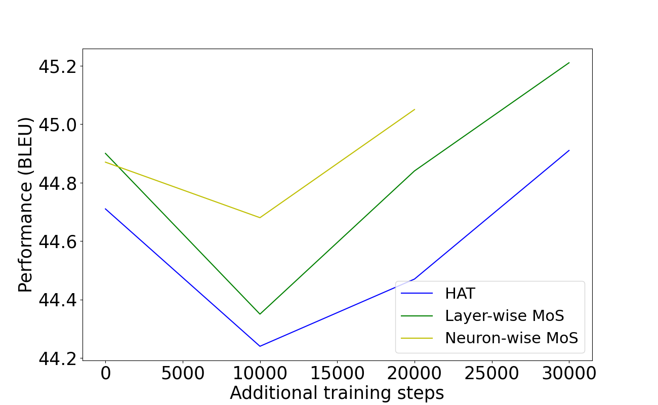
Figure 4, Figure 5, and Figure 6 show the additional training steps vs. BLEU for different latency constraints on the WMT’14 En-De task, WMT’14 En-Fr and WMT’19 En-De tasks respectively.


A.5.6 Evolutionary Search - Stability
We study the initialization effects on the stability of the pareto front outputted by the evolutionary search for different supernets. Table 14 displays sampled (direct) BLEU and latency of the models in the pareto front for different seeds on the WMT’14 En-Fr task. The differences in the latency and BLEU across seeds are mostly marginal. This result highlights that the pareto front outputted by the evolutionary search is largely stable for all the supernet variants.
| Supernet / Pareto Front | Model 1 | Model 2 | Model 3 | ||||
|---|---|---|---|---|---|---|---|
| Seed | Latency | BLEU | Latency | BLEU | Latency | BLEU | |
| HAT (SPOS) | 1 | 96.39 | 38.94 | 176.44 | 39.26 | 187.53 | 39.16 |
| HAT (SPOS) | 2 | 98.91 | 38.96 | 159.87 | 39.20 | 192.11 | 39.09 |
| HAT (SPOS) | 3 | 100.15 | 38.96 | 158.67 | 39.24 | 189.53 | 39.16 |
| Layer-wise MoS | 1 | 99.42 | 39.34 | 158.68 | 40.29 | 205.55 | 41.24 |
| Layer-wise MoS | 2 | 99.60 | 39.32 | 156.48 | 40.29 | 209.80 | 41.13 |
| Layer-wise MoS | 3 | 119.65 | 39.32 | 163.17 | 40.36 | 208.52 | 41.18 |
| Neuron-wise MoS | 1 | 97.63 | 39.55 | 200.17 | 40.02 | 184.09 | 41.04 |
| Neuron-wise MoS | 2 | 100.46 | 39.55 | 155.96 | 40.04 | 188.87 | 41.15 |
| Neuron-wise MoS | 3 | 100.47 | 39.57 | 157.26 | 40.04 | 190.40 | 41.17 |
| # layers in router function | BLEU () |
|---|---|
| 2-layer | 26.61 |
| 3-layer | 26.14 |
| 4-layer | 26.12 |
A.5.7 Impact of different router function
Table 15 displays the impact of varying the number of hidden layers in the router function for neuron-wise MoS on the WMT’14 En-De task. Two hidden layers provide the right amount of router capacity, while adding more hidden layers results in steady performance drop.
A.5.8 Impact of increasing the number of expert weights ‘m’
Table 16 displays the impact of increasing the number of expert weights ‘m’ for the WMT’14 En-Fr task, where the architecture for all the supernets is the top architecture from the pareto front of HAT for the latency constraint of ms. Under the standard training budget ( steps for MT), the performance of layer-wise MoS does not seem to improve by increasing ‘m’ from 2 to 4. Increasing ‘m’ introduces too many parameters, which might necessitate a significant increase in the training budget (e.g., 2 times more training steps than the standard training budget). For fair comparison with existing literature, we use the standard training budget for all the experiments. We will investigate the full potential of the proposed supernets by combining larger training budget (e.g., steps) and larger number of expert weights (e.g., expert weights) in future work.
| Supernet | m | BLEU () | Supernet GPU Memory () |
|---|---|---|---|
| HAT | - | 39.13 | 11.4 GB |
| Layer-wise MoS | 2 | 40.55 | 15.9 GB |
| Layer-wise MoS | 4 | 40.33 | 16.1 GB |
A.5.9 SacreBLEU vs. BLEU
We use the standard BLEU (Papineni et al., 2002) to quantify the performance of supernet following HAT for a fair comparison. In Table 17, we also experiment with SacreBLEU (Post, 2018), where the similar trend of MoS yielding better performance for a given latency constraint holds true.
| Supernet | BLEU () | SacreBLEU () |
|---|---|---|
| HAT | 26.25 | 25.68 |
| Layer-wise MoS | 27.31 | 26.7 |
| Neuron-wise MoS | 27.59 | 27.0 |
A.5.10 Breakdown of the overall time savings
Table 18 shows the breakdown of the overall time savings of MoS supernets versus HAT for computing pareto front for the WMT’14 En-De task. The latency constraints include ms, ms, ms. MoS have an overall GPU hours savings of at least 20% w.r.t. HAT, thanks to significant savings in additional training time (45%-51%).
| Supernet | Overall Time () | Supernet Training Time () | Search Time () | Additional Training Time () |
|---|---|---|---|---|
| HAT | 508 hours | 248 hours | 3.7 hours | 256 hours |
| Layer-wise MoS | 407 hours (20%) | 262 hours (-5.6%) | 4.5 hours (-21.6%) | 140 hours (45.3%) |
| Neuron-wise MoS | 394 hours (22%) | 266 hours (-7.3%) | 4.3 hours (-16.2%) | 124 hours (51.6%) |
A.5.11 Codebase
We share the codebase at: https://github.com/UBC-NLP/MoS, which can be used to reproduce all the results in this paper. For both BERT and machine translation evaluation benchmarks, we add a README file that contains the following instructions: (i) environment setup (e.g., software dependencies), (ii) data download, (iii) supernet training, (iv) search, and (v) subnet retraining.