MIXING LAYER AND TURBULENT JET FLOW
IN A HELE–SHAW CELL
Abstract
A plane turbulent mixing in a shear flow of an ideal homogeneous fluid confined between two relatively close rigid walls is considered. The character of the flow is determined by interaction of vortices arising at the nonlinear stage of the Kelvin–Helmholtz instability development and by turbulent friction. In the framework of the shallow water theory and a three-layer representation of the flow, one-dimensional models of a mixing layer are proposed. The obtained equations allow one to determine averaged boundaries of the region of intense fluid mixing. Stationary solutions of the governing equations are constructed and analysed. Using the averaged flow characteristics obtained by one-dimensional equations, a hyperbolic system for determining the velocity profile and Reynolds shear stress across the mixing layer is derived. Comparison with the experimental results of the evolution of turbulent jet flows in a Hele–Shaw cell shows that the proposed models provide a fairly accurate description of the average boundaries of the region of intense mixing, as well as the velocity profile and Reynolds shear stress across the mixing layer.
keywords:
shallow water equations; mixing layer; jet flow; Hele–Shaw cell1 Introduction
The interaction of fast and slow flows when they merge leads to the appearance of vortex structures and the formation of a mixing layer [3, 24, 11]. Interest in modelling of such flows is associated with geophysical and technical applications, in which there is a need to describe the mixing processes during the confluence of rivers or streams in open and closed channels. For a wide class of flows, the study of shear instability can be carried out in the framework of the two-dimensional shallow water theory, taking into account the effect of bottom friction. In this case, the character of the quasi-two-dimensional flow and the mixing intensity are determined by interaction of vortices arising at the nonlinear stage of the Kelvin–Helmholtz instability and by friction caused by a small thickness of the fluid layer. Note that the fluid motion between two relatively close rigid walls can be interpreted as a flow in a Hele–Shaw cell with the law of friction on the walls corresponding to the turbulent flow regime. The study of such shear flows becomes relevant in the problems of underground hydrodynamics in modelling hydraulic fracturing.
Laboratory experiments on the formation and evolution of plane turbulent mixing layer for free surface flows were performed in [7, 29]. These results allowed one to obtain empirical formulas for estimating the size of the mixing area as well as determine the parameters at which the flow is stabilized and the growth of the intermediate mixing layer stops. In [25, 28] the field observations of confluent streams were discussed and compared with some theoretical results. Mathematical models of the plane mixing layer development based on the averaged equations of the shallow water theory were presented and verified in [2, 21]. The characteristic features of the development of mixing layers in shallow water at various flow parameters were numerically studied in [19, 12]. Theoretical and experimental study of quasi-two-dimensional processes of turbulent mixing in flows between rigid walls also attracts the attention of researchers. An experimental study and numerical simulation of the evolution of submerged jets in a Hele–Shaw cell were carried out in [22, 23], where the formation of large vortex structures and meanders at Reynolds numbers of the order of were discussed. Here it was assumed that the width of the jet in the inlet section significantly exceeded the thickness of the channel. In works [13, 14], on the contrary, flows are considered in which the width of the jet in the inlet section is smaller than the thickness of a Hele–Shaw cell. Experimental results on the meandering of turbulent jets were presented and a theoretical estimate for determining the averaged jet boundaries was given. The asymptotic theory of secondary steady flow in turbulent mixing layers was developed in [30].
Improving the models of shear fluid flow is caused by the necessity of describing the nonlinear stage of the Kelvin–Helmholtz instability development and adequate modelling of a turbulent mixing in the framework of averaged equations of motion. In works [18, 16] an original method was proposed for constructing one-dimensional models for the propagation of nonlinear perturbations in the shear flow of a thin fluid layer. This method is based on the application of the theory of three-layer shallow water taking into account turbulent mixing in the intermediate layer. Implementation of the method allows for two different approaches. The first of them is based on averaging the Reynolds equation of the turbulent flow over the channel width with the additional assumption that the Reynolds shear stress is proportional to the specific kinetic energy of the fluctuating motion [15, 17]. The second one uses the procedure proposed in [26] for averaging shallow water equations for shear flows [1, 5]. It was applied to construct a three-layer model of horizontal mixing in fairly deep fluid flows in open channels [20]. In [4], this model was improved by taking into account bottom friction and verified by comparison with experimental data [2] and the results of numerical simulations based on two-dimensional equations of shallow water theory. The same approach was successfully applied in [9] to simulate the breaking of surface long waves taking into account the effects of vorticity and dispersion. Note that despite the differences in the derivation of 1D models of the mixing layer, the obtained equations of motion have a similar structure and, as a rule, give close quantitative results [16].
The purpose of this work is to derive, analyse and verify one-dimensional models describing the formation and evolution of the mixing layer in a shear flow of a homogeneous fluid confined between two relatively close parallel walls. Construction of the models is based on a three-layer representation of the flow taking into account turbulent mixing. In the next section, we derive 1D models for describing the mixing layer applying the Reynolds equations for turbulent flows (Model I) and the shallow-water equations for shear flows (Model II). Both models have a similar structure and allow a uniform presentation. The equations of motion include two empirical parameters responsible for mixing and dissipation of energy. In section 3, we construct and study stationary solutions. We show that the boundaries of the mixing layer obtained by Models I and II almost coincide. Then we show that the boundaries of the region of intense mixing for Hele–Shaw jet flows obtained from the proposed models are in good agreement with experimental data. Using the solution of the averaged 1D equations of motion, we derive a hyperbolic system for determining the velocity profile and Reynolds shear stress across the mixing layer. The results of calculating the velocity profile and shear stress are verified by comparison with the experimental data. In section 4, we modify these 1D models for the case of shear flows without a pressure gradient. Such models, in particular, are used to describe a submerged jet in an infinitely wide channel. A comparison of the calculation results utilizing stationary equations of motion with the available experimental data indicates the possibility of using these models to determine the averaged boundaries of a turbulent jet. Finally, we draw some conclusions.
2 Governing equations
In the shallow water approximation, a spatial flow of a homogeneous ideal fluid under a rigid-lid (in a Hele–Shaw cell) is described by the equations
| (1) |
Here and are the spatial variables; is the time; and are the velocity vector components; is the ratio of the pressure at the rigid-lid to the fluid density ; factor is the ratio of the friction coefficient to the channel thickness . It supposes that in the plane the flow region is bounded by the rigid walls and . Therefore, we supplement Eqs. (1) with the boundary conditions
| (2) |
The obvious consequence of system (1) is the energy equation
| (3) |
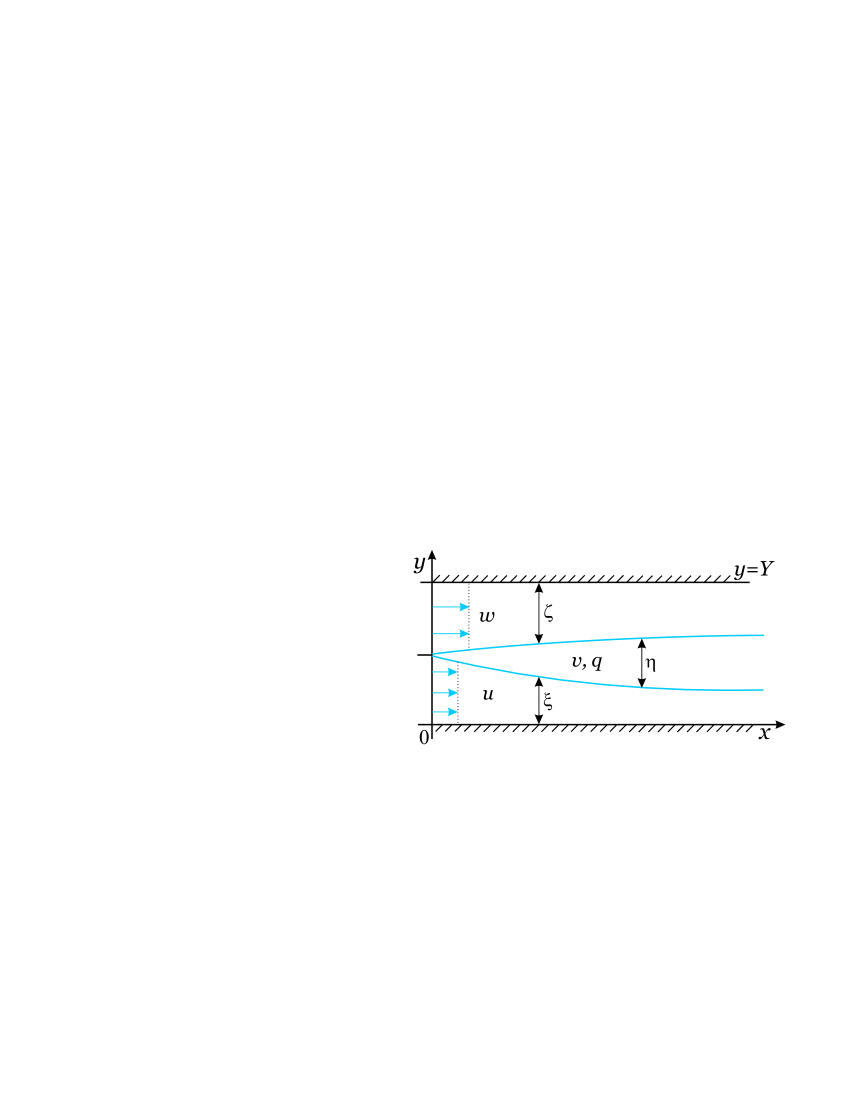
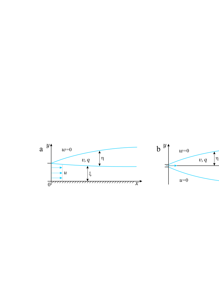
We consider the problem of the formation of a mixing layer in the confluence of two weakly shear flows. In the framework of the three-layer flow scheme (see Fig. 1) we derive one-dimensional system of equations describing the evolution of the mixing layer. Let , and denote the width of the outers and intermediate layers. The average flow velocities in these domains are , , and , respectively. In the outer layers, the flow is assumed to be slightly shear and can be described using average velocities: for , for . A vortex flow is realized in the mixing layer. Therefore, in addition to the average flow velocity another variable is introduced. This quantity characterizes the spatial inhomogeneity of the flow (and will be defined below). It is assumed that the fluid motion mainly occurs in the direction of the axis and the ratio of the characteristic transverse scale of the flow to the longitudinal scale of is small . For convenience of further calculations we assume .
As a result of averaging of Eqs. (1) over the channel width with the above-mentioned assumptions, the following system is obtained
| (4) |
Here is the fluid flow rate (referred to the channel thickness ); constant ; non-negative constants and are the empirical parameters responsible for mixing between layers and energy dissipation; the coefficient takes values 0 and 1, which corresponds to Models I and II. In both cases, Eqs. (4) form a closed system for determining the width of the layers , , and , the average fluid velocity in these layers , , and , the pressure , and the variable . Let us proceed to the derivation of Eqs. (4).
2.1 Derivation of Model II
We perform the following scaling in Eqs. (1) and (3)
Then we neglect all terms of the order of . As a result, we obtain the equations of the horizontal-shear flow of a thin fluid layer in a closed channel
| (5) |
The last equation in (5) is a consequence of the first three ones. We supplement system (5) with boundary conditions (2).
Let us assume that the velocity profile satisfies the condition
| (6) |
with the parameters and . To describe a three-layer flow, we introduce the averaged velocities in the layers and the root-mean-square deviation (shear velocity ) in the intermediate layer:
| (7) |
The process of fluid involvement in the vortex interlayer is assumed to be symmetric and is taken into account by kinematic conditions at the internal boundaries
| (8) |
This means that the rate of fluid entrainment into the vortex interlayer is proportional to the velocity of “large eddies” generated in the vicinity of the interface between the layers due to shear instability [4, 9]. According to [18], the proportionality coefficient is approximately equal to .
In averaging Eqs. (5) over the channel width the necessity of approximate calculation of the integrals of the functions () with respect to the variable arises. The following estimates are valid for weakly-shear layers:
As terms of the order of are ignored in deriving model (5), the velocity is replaced in the course of averaging the equations of motion in the weakly shear layers by the corresponding averaged values of and determined by formulas (7). Using the obvious identity , we calculate the integrals in the intermediate mixing layer:
| (9) |
Condition (6) implies the estimate , . Therefore, the value of is small compared to other terms and can be omitted [26].
The fulfilment of conditions (6) imposed on the velocity profile is sufficient to require at the initial moment of time . Indeed, by virtue of (5), the variable satisfies the equation
and, consequently, decreases with time.
With allowance for the adopted assumptions, as a result of averaging Eqs. (5) over the channel width and using boundary conditions (2) and (8), we obtain system (4) for (Model II). The first three equations of system (4) express the mass balance in the layers. Since then the flow rate does not depend on the cross section, i.e. . The fourth and fifth equations are the local momentum conservation laws in the outer layers, the sixth and seventh equations are the total momentum and energy conservation laws. The last term in the energy equation with the factor does not directly follow from the averaging over the channel width of the last equation in (5). It is added to take into account the energy dissipation. According to [18], the numerical value of the empirical parameter lies in the interval from 2 to 8.
Governing equations (4) imply the fulfilment of the conditions
They are the consequence of the compatibility of the equations of balance of mass, momentum and energy in weakly-shear layers. A similar approach for determining the velocity at the interface was used in [4, 9]. Indeed, averaging Eqs. (5) over the width of one of the outer layers yields the system
| (10) |
Averaging over another weakly-shear layer gives the same equations up to the replacement of , and with , and . It is easy to show that the compatibility of system (10) for is ensured by the condition .
2.2 Derivation of Model I
At large Reynolds numbers, vortex motions of various scales arise as a result of the development of shear instability. Let a certain scale be chosen and a procedure for averaging the unknown variables be constructed. Then the velocity field and pressure can be represented as
| (11) |
where , and are the average velocity components and pressure; , and are the corresponding fluctuations relative to the average variables such that . We substitute representation (11) into system (1) and energy equation (3). After averaging over the selected scale, we obtain the Reynolds equations:
| (12) |
Here is the Reynolds shear stress; is the total pressure; is the specific kinetic energy of the fluctuating motion. On the right-hand sides of Eqs. (1), the true velocities are replaced by their average values without fluctuating terms. In deriving Eqs. (12) an assumption is made about the isotropy of the fluctuating motion, i.e. . Moreover, the terms , and () having a higher order of smallness compared to are neglected. The last term in the fourth equation (12) is added to take into account the outflow of energy into small-scale motion. The characteristic frequency is responsible for the energy dissipation rate of turbulent motion. In view of condition (2) on the side walls of the channel and the velocity component vanishes.
In a developed turbulent flow the following dependence for the Reynolds shear stress was experimentally confirmed in [27]
| (13) |
Eqs. (12), (13) are the closed system for determining the functions , , and . Taking into account that the fluid moves mainly along the axis, we proceed to the approximation of a long channel (). We assume here that the fluctuating components , and the variable are of the same order. Then the following scaling
| (14) |
in Eqs. (12) and neglecting the leading terms in powers of the small parameter yields
| (15) |
where is defined by formula (13). Following [18], we assume . It should be noted that in scaling (14) the value has the same order of smallness as the parameter , therefore, the terms are kept in Eqs. (15). Further, in Eqs. (15) we take .
Let us average Eqs. (15) over the channel width taking into account a three-layer representation of the flow (Fig. 1). We assume that in the outer weakly-shear layers of width and there is no kinetic energy of fluctuating motion (), and the flow velocity is equal to and , respectively. In the intermediate mixing layer of width we replace velocity by its average value and denote the average value of the function . We recall that upon obtaining Eqs. (12) (and (15)), a certain averaging scale is fixed. If, as such a scale, we choose the width of the mixing layer , then . In view of the second equation in (15) the total pressure is . At the interfaces and , it is assumed that kinematic conditions (8) are satisfied (with velocities and instead of and ). As a result of averaging Eqs. (15) over the channel width, we obtain system (4) for (Model I).
2.3 Transformation of Eqs. (4)
For further analysis of the equations of motion and the construction of stationary solutions it makes sense to derive some consequences. By virtue of system (4) the variables , and satisfy the equations
| (16) |
Using the sixth equation in system (4) we eliminate , replace the energy equation with the differential consequence for the variable , and also express and in terms of other variables. Then system (4) is transformed to the following equations to determine five unknowns , , , and :
| (17) |
Here function is defined in the last formula (16), the variables , and are expressed as follows:
The flow rate is considered to be given. The pressure on the rigid-lid is found from the fourth or fifth equation of system (4). As it was mentioned above the coefficient for Model I and in the case of Model II. Eqs. (17) is used below for an averaged description of the mixing layer.
2.4 Characteristics of Eqs. (17)
Let us represent Eqs. (17) in the form
where is the vector of unknown variables, and is the corresponding matrix of size and the right-hand side vector. The eigenvalues of matrix determine the propagation velocity of the characteristics. By virtue the last equation in system (17), Model I () has the contact characteristic . Model II () has the same characteristic since equation holds on for the variable (here the right-hand side term does not contain derivatives of the unknown functions). To determine the others characteristics of system (17), an algebraic equation of the fourth degree arises
The case corresponds to the initial point of confluence of two flows of the same width. The polynomial is simplified and takes the form
For both models ( and ), equation has two complex and two real roots. It is necessary to note that in the framework of Model I, all real characteristics are contact and propagate with the average velocity in the intermediate mixing layer. Thus, the system under consideration is not hyperbolic in the vicinity of the confluence of flows. It is associated with the development of the Kelvin–Helmholtz instability at the interface.
Remark 1
As it is shown in [4] a similar to model (4) system of equations describing a mixing layer for horizontal-shear flow with a free surface has, at least, three real characteristics (one contact and two sonic ones). Moreover, under certain conditions this system is hyperbolic, that allows one to use standard numerical methods developed for solving hyperbolic equations. A modification of system (4) for shear flows of a weakly compressible barotropic fluid under a rigid-lid also has real sonic characteristics and consequently can be used to model non-stationary processes in mixing layers.
3 Stationary solutions
The steady-state fluid flows in the framework of three-layer model (17) are determined by solving the system of ODE
We denote by “prime” the derivative with respect to . After some transformations the system is rewritten in the normal form:
| (18) |
Here
the function is the right-hand side in the last equation in (16), the coefficient takes values 0 and 1 (Models I and II, respectively).
3.1 Initial section of the mixing layer
The equations describing a stationary mixing layer are derived above. To construct the solution, it is necessary to impose the conditions at the point of mixing layer formation, i.e., to find the asymptotic of the stationary solution (18) as . Without loss of generality, we assume that at , and the values of the functions at this point are marked by the zero subscript. Let at the parameters of weakly shear layers , , and be specified (all values are positive). We assume that there are finite limits of the functions , as and find these values.
By virtue of the last two equations in (16) and (in the case ) the second equation in (4) we have the relations
| (19) |
For model I () it follows from the first equation in (19) that and from the second equation in (19) the value of is determined. For model II () relations (19) are reduced to the quadratic equation for determining
Here we denote . This equation has two real roots for all if , where . From the two roots and , we choose the closest to the value of . If tends to unity (the velocities of the merging flows and are close), then the region of existence of the quadratic equation solution with respect to the parameter expands. The indicated restriction on the choice of the dissipation parameter should be taken into account in calculations according to Model II.
3.2 Stationary mixing layer
We obtain a numerical solution of Eqs. (18) for the parameters of the incoming flow taken from [2] (case A): m/s, m/s. The calculations are performed for a straight channel having 16 m long and 3 m wide. Its depth is equal to 0.052 m. We assume m, and . For this and all subsequent tests, we choose . The solution of the stationary mixing layer problem is not difficult, since it is described by a system of ordinary differential equations. The calculations are carried out in the MATLAB environment using the ode45 function that implements the fourth-order Runge–Kutta method.
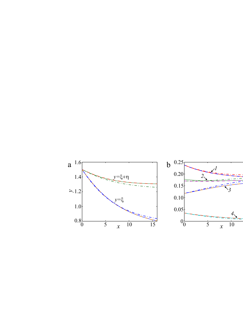
Let two streams moving with the above-given velocities and merge in the cross section , where an intermediate mixing layer is formed. For the chosen flow parameters at , formulas (19) uniquely determine the values and . For Model I we have , for Model II — ; in both cases . The results of calculation using Eqs. (18) are shown in Fig. 2 by solid curves (Model I) and dashed lines (Model II). As can be seen from the graphs, in this example, Models I and II give almost the same result. A slight difference in the calculations for these models is observed only for the velocity at the initial stage of the mixing layer formation. This is due to the difference in definitions of and by formulas (19) for and . Dashed-dotted lines in Fig. 2 correspond to the similar solution (in the framework of Model II) for the flow in an open channel. The solution is obtained in [4] and verified by experimental data [2]. Comparison of the calculating results of the mixing layer evolution for shear flows in open and closed channels is not entirely correct. Nevertheless, at the initial stage of the mixing layer formation, a good agreement between the solutions of the equations describing the flows under a rigid-lid and with a free surface is observed.
Remark 2
Remark 3
Eqs. (4) (and (18)) include the empirical parameters and , which are responsible for the entrainment of fluid from the outer layers into the intermediate mixing layer and energy dissipation. A small variation of these parameters leads to a small change in the solution. The detailed analysis of the influence of the variations and for two-layer flows with mixing in open channels is given in [6].
3.3 Jet flow in a Hele–Shaw cell
The calculation results using Eqs. (18) for Models I () and II () practically coincide if the ratio of the flow velocities in the input section satisfies the inequality . As a rule, for problems of jet flows one of the outer fluid layers is at rest. Therefore, the relation (or ). In this case, the determination of and from relations (19) for is possible only for sufficiently large values of the dissipation parameter . In addition, in the framework of Model II, the value of differs markedly from the half-sum of the outer layers velocities . For this reason, in such problems to apply Model I is preferable. To avoid the singularity in Eqs. (18), the fluid velocity in the resting layer is assumed to be positive, but close to zero.
The mixing layer boundaries obtained by the proposed model are in a good agreement with the experimental data and the results of direct numerical simulation performed in [22, 23] for jet Hele–Shaw flows at the Reynolds numbers of the order of . We consider jet flow in a closed channel of the size (corresponds to the directions ), where mm, and . The channel is filled with fluid at rest. Through a slot of width located in the centre of the cross-section a fluid with velocity m/s is supplied [23]. Below we use this velocity as a scale for the mixing layer reconstruction. Therefore, in dimensionless variables, the jet velocity is chosen equal to one. To visualize the fluid flow at the boundaries of the inlet section, the colouring fluid is injected using needles. As a result of the development of Kelvin–Helmholtz instability, turbulent mixing layers are formed at the interfaces between the jet and the fluid at rest.
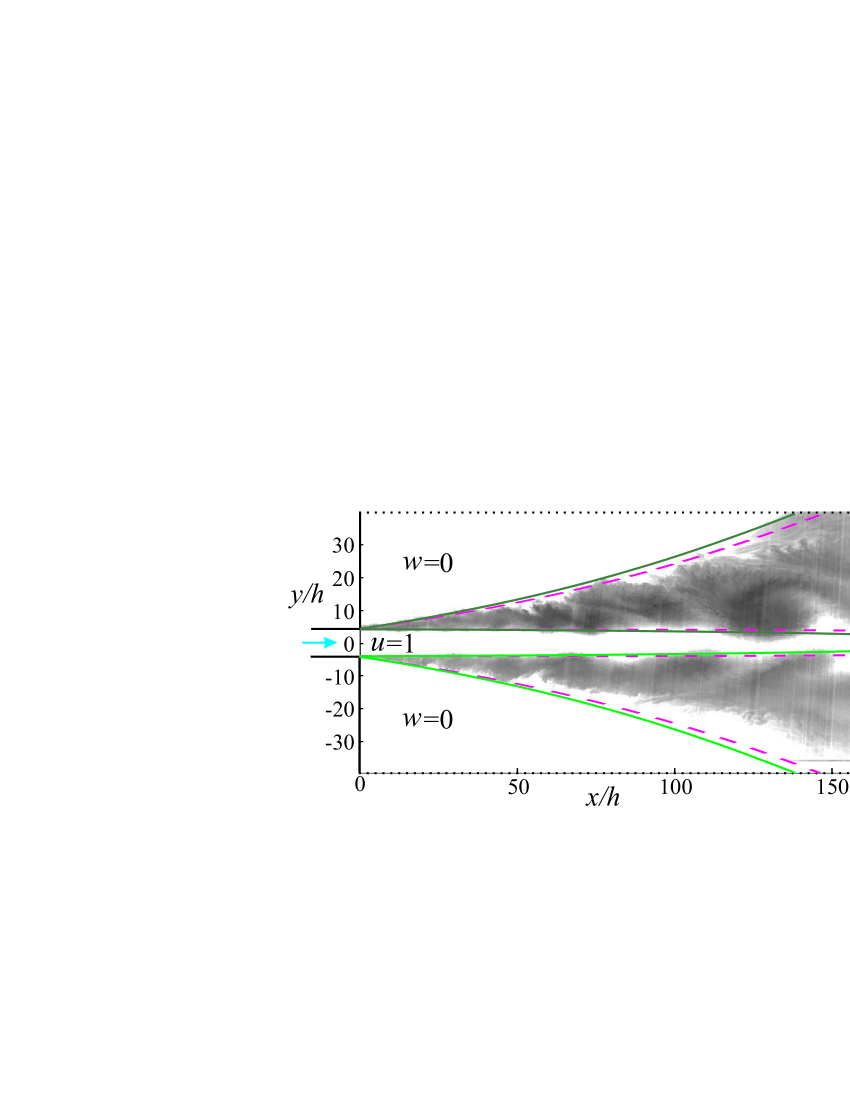
Let us choose the following parameters , , , , and compute the mixing layer boundaries and using Eqs. (18) with (Model I). The channel thickness is chosen as the flow scale. The values of the empirical parameters are , . According to [8] the friction coefficient of the two-dimensional rectangular duct flow can be found as
| (20) |
Therefore, for flows with the Reynolds numbers of the order of considered in [23], the friction coefficient is .
Boundaries of the mixing layer and obtained by Eqs. (18), as well as a symmetric about the axis solution corresponding to the conditions , and , are shown in Fig. 3. Solid curves correspond to the dissipation parameter , dashed lines — . The results of these calculations are overlaid on the grey-scaled picture of a turbulent jet presented in [23] (Fig. 3, d). It should be noted that the region of intense mixing mainly propagates into the layer of the fluid at rest and the distance between the internal boundaries of the mixing layers does not decrease until the stability of the jet is lost. As can be seen from Fig. 3, Eqs. (18) make it possible to determine the boundaries of intense mixing region in a Hele–Show jet flow without time-consuming calculations on the basis of 2D or 3D equations.
3.4 Velocity profile and shear stress across the mixing layer
Let a solution of Eqs. (18) be constructed in the framework of Model I or II. Below we show that this solution can be applied to determine the velocity profile and Reynolds shear stress across the mixing layer. For this goal, we use stationary equations (15) taking into account the intermittency of the flow (irregularity of the layer boundaries in a turbulent flow), we set (see [15] and [18], Ch. 7)
The functions , and are considered as known ones. They are determined by the solution of stationary Eqs. (4). Under the above-mentioned assumptions, Eqs. (15) for steady flows take the form
| (21) |
To analyse this system, it is convenient to pass to the Mises variables , where is the stream function associated with the velocity field by relations , .
We denote
and take into account that
(derivatives of the functions and are calculated in the similar way). Then Eqs. (21) in the variables are transformed to the semi-linear hyperbolic system with respect to the variable :
| (22) |
The characteristics of system (22) are given by the equations . The problem is similar to that considered in [18, 5] for a plane-parallel shear flow in a channel of finite thickness (flow with a pressure gradient). This is formulated for Eqs. (22) in the form of the Goursat problem with data on the characteristics. The difference consists only in the modification of the right-hand side (22) related to the consideration of friction. Solution of Eqs. (22) is constructed numerically using a Godunov-type scheme. Then, the velocity profile is obtained as a result of integration of the equation and the transition to the original variables .
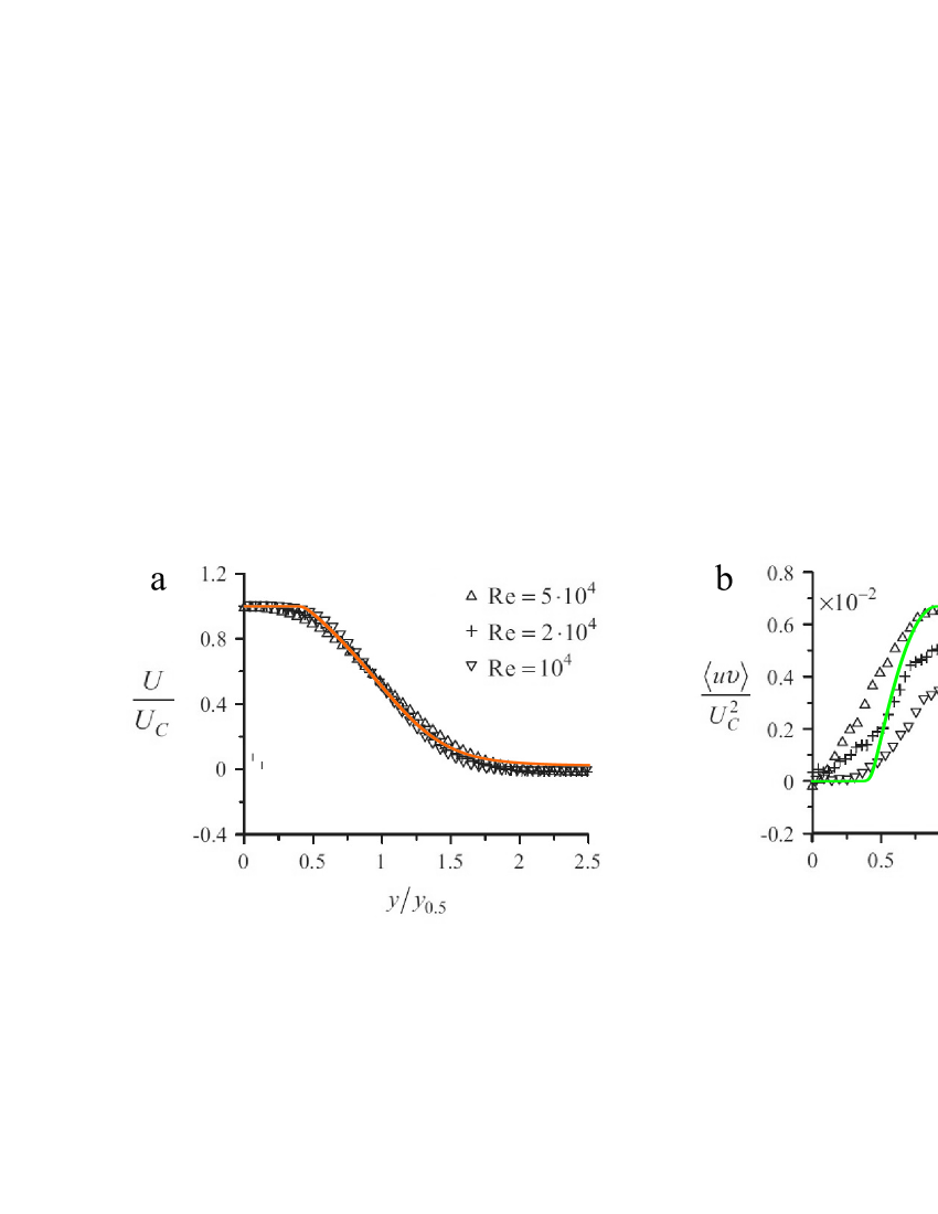
The results of experimental measurements of the velocity profile and Reynolds shear stress are given in [22]. This work considers a turbulent jet flow between two parallel plates (separated by a distance ) issuing from a rectangular nozzle (with a span-wise size ) in the stream-wise direction . Fig. 3 in [22] presents the measurement results for jet flows with , and obtained for at the cross-section . Here is the virtual origin of the jet ( for ). The velocity profiles and Reynolds stresses presented in [22] are normalized to and , respectively. Here is the centreline velocity in the far jet field taken in the form [10]
| (23) |
with and .
To carry out the calculations based on Eqs. (18) (Model I) and then using Eqs. (22), we choose , , , and . The empirical parameters are as follows: , and . We also assume . The calculation results (functions and normalized to the jet velocity and ) are shown in Fig. 4 by solid curves at the cross-section . The value is chosen so that for . As can be seen from Fig. 4, the calculation results for the proposed models are in a good agreement with experimental data [22]. We note that outside the mixing layer, and coincides with the external velocity (for ) or (for ). Since we take to avoid singularity in the governing equations, on the right border of Fig. 4 (a) the calculated velocity profile is slightly higher than the experimental values. The condition is fulfilled everywhere in the flow. The Reynolds shear stress practically coincides with the data from [22] for in the region . The differences for can be associated with meandering and penetration of vortices into the central part of the jet.
![[Uncaptioned image]](https://cdn.awesomepapers.org/papers/e0d96704-c7db-439d-8092-3d03f9c3dc5c/x5.png)
![[Uncaptioned image]](https://cdn.awesomepapers.org/papers/e0d96704-c7db-439d-8092-3d03f9c3dc5c/x6.png)
Fig. 6 presents the stream-wise velocity in the centre of the jet. It follows from Fig. 6 that the centreline velocity in the far-field given by the empirical formula (23) has the similar behaviour as the velocity calculated by Eqs. (18) for . At the considered cross-section these values almost coincide. Thus, using the solution of Eqs. (18), we can obtain the transverse distribution of the velocity profile and Reynolds shear stress in the mixing layer on the basis of hyperbolic Eqs. (22).
4 Hele–Shaw flow without pressure gradient
Let us consider the fluid motion in a closed channel of thickness and unlimited width (the side wall is considered to be infinitely distant). It corresponds to a flow without a pressure gradient. Further we show that such reduced models can be used to describe at least the initial stage of the stationary mixing layer (Fig. 6). As before, we assume that the channel is occupied by the fluid at rest. Through a slot of width at a fluid with constant velocity is injected into the channel. The flow scheme is shown in Fig. 7 (a). Taking and in Eqs. (4), we obtain the following system for determining unknown functions , , , and :
| (24) |
Here we choose (i.e., Model I) to describe Hele–Shaw jet flows. The consequence of system (24) are Eqs. (16). In these equations we should put and . According to the above-mentioned consequences, stationary equations (24) take the form
| (25) |
where . At the starting point of the mixing layer formation due to conditions (19), we have , . It should be pointed out that the presence of two integrals
allows one to reduce Eqs. (25) to a system of two ODEs.
Boundaries of the mixing layer and ) obtained by Eqs. (25) for , , , , and are shown in Fig. 6 (dashed curves). For the calculation according to Eqs. (18) (Model I) we additionally put and . The result of the calculations is shown in the same figure (solid curves). As we can see, at a distance of the order of 160 from the input section of the channel, the mixing layer boundaries practically coincide for the considered models. Therefore, Eqs. (25) without a pressure gradient can be used to describe (at least) the initial stage of the mixing layer development for jet flows in a Hele–Shaw cell.
4.1 Turbulent jet in a Hele–Shaw cell
We consider a quasi-two-dimensional plane turbulent jet discharged from a slot of width into a fluid confined between two relatively close plane parallel walls with gap . Let us try to describe the averaged boundaries of the jet in the framework of stationary solution of Eqs. (24) without taking into account the pressure gradient. The fluid velocity in both outer layers is equal to zero. The sketch of the flow is shown in Fig. 7 (b). Assuming symmetry with respect to the centre line of the channel , stationary equations (24) can be written as
Let us transform these equations to the normal form
| (26) |
If we neglect the friction (), then Eqs. (26) have the following exact solution
| (27) |
where is the positive constant, and . Without loss of generality, we take and, as before, we choose .
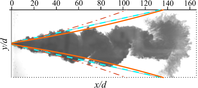
Theoretical and experimental study of steady quasi-two-dimensional plane turbulent jet flows was performed in [13, 14]. The self-similar character of the jet spreading at the initial stage is reported in these works. Let us compare the results of calculations of the averaged jet width according to Eqs. (26) with the experimental data [14] obtained in a Hele–Shaw cell of thickness , length and width . For the jet flow considered in [14] (see Fig. 9 (a) in the cited work), the half-spreading angle of the jet is as follows . This means that in formula (27) constant is equal to . Because the width of the input section is , so that . Hence, we find the virtual origin of the self-similar jet , as well as the values and . Due to the relationship between , and we define the value of . The straight line and symmetrical to it relative to the centre line of the channel are shown in Fig. 8 by dashed curves. These lines coincide with the average dye edges plotted in [14] (Fig. 9 (a)).
Presented in [14] grey-scale picture of a dyed jet rising in the tank was obtained for . Therefore, according to empirical formula (20) proposed in [8], we take the friction coefficient to calculate the average width of the turbulent flow using Eqs. (26). Solid curves in Fig. 8 are the solution of Eqs. (26) with the above pointed data at and the dissipation parameter . This solution gives a slightly smaller width of the turbulent flow region compared to the self-similar solution (27). Dash-dotted curves in the figure represent the solution of Eqs. (26) obtained for and . This solution has the correct asymptotic behaviour near the inlet cross-section, but in the far field gives an overestimated value of the average jet width. Thus, comparison with Fig. 9 (a) in [14] shows that Eqs. (26) allow one to determine the average boundary of a turbulent jet flow in a Hele–Shaw cell.
5 Conclusion
One-dimensional models of the formation and evolution of a mixing layer in shear shallow flows of a homogeneous fluid under a rigid-lid (in a Hele–Shaw cell) are proposed. The construction of these models is based on averaging over the channel width of the two-dimensional Reynolds equations with an additional closure condition (Model I) or a quasi-two-dimensional system of equations of shear fluid flow with internal boundaries (Model II). In both cases, the obtained equations of motion are based on a three-layer representation of the flow, taking into account the fluid entrainment process from the outer regions of weakly-shear flow into the vortex interlayer (Fig. 1). The rate of fluid entrainment in the mixing layer is proportional to the “large billows” velocity generated in the vicinity of the layer interface. The obtained models are written in a unified way and presented in the form of system of five evolution equations (17) for determining the layers width and average velocities in them, as well as an additional variable responsible for the mixing process. Both models include two empirical constants and . The first one is responsible for the mixing intensity and the second one for energy dissipation. For all tests we choose , while is varied from 5 to 8. It should be note that for shear flows in open channels [9, 16, 4] more precise coincidence with experimental data is observed for and the same parameter .
The main attention in this paper is paid to the study of stationary solutions. The governing equations are transformed to normal form (18). Stationary solution to the problem of a mixing layer in shallow water under a rigid-lid is obtained and the comparison is made with a similar problem for flows in an open channel (Fig. 2). If the ratio of velocities in the outer layers differs from unity by less than four times, then Models I and II give almost the same result. Moreover, the initial stage of mixing for flows under a rigid-lid and with a free surface practically coincides. Model I (Eqs. (18) with ) is more suitable for describing flows in which the velocity of one of the outer layers is close to zero. In this case, according to (19) there is no difficulty in determining the flow parameters at the initial point of the mixing layer formation. This model is verified by comparison with experimental data obtained in [23] for turbulent Hele–Shaw jet flows. Fig. 3 shows the results of visualization of the mixing layers when the jet interacts with the fluid at rest as well as the boundaries of the regions of intense mixing calculated using Model I. Further, it is shown that the constructed solution of the averaged equations within a three-layer representation of the flow can be used to obtain the velocity profile and turbulent shear stress across the mixing layer. For this goal, the Reynolds equations in the form (21) are used. In the Mises variables, these equations reduce to a semi-linear hyperbolic system (22). Numerical solution of these equations allow one to obtain the velocity profile and Reynolds shear stress across the mixing layer. The calculation results are verified by the experimental data [22] (see Fig. 4 and 6).
Modification of the derived averaged equations for shear flows without a pressure gradient (24) is considered. This corresponds to quasi-two-dimensional flows with internal boundaries in a channel of unlimited width (see Fig. 7). A comparison of the mixing layer boundaries obtained by Eqs. (18) and (24) shows, the model without taking into account the pressure gradient is applicable, at least, to describe the initial stage of the mixing layer (Fig. 6). In the framework of two-layer equations (26), the boundaries of the turbulent submerged jet in a Hele–Shaw cell are determined. The calculation results are in a good agreement with experimental data [14] presented in Fig. 8. Verification of the models indicates the possibility of their application for an averaged description of jet flows and determination of the boundaries of the large vortex structures formation.
Acknowledgements
This work was partially supported by the Russian Foundation for Basic Research (project 19-01-00498).
References
- [1] D.J. Benney, Some properties of long nonlinear waves, Stud. Appl. Math. 52 (1973) 45–50.
- [2] R. Booij, J. Tukker, Integral model of shallow mixing layer, J. Hydraul. Res. 39 (2001) 169–179.
- [3] G.L. Brown, A. Roshko, On density effects and large structure in turbulent mixing layers, J. Fluid Mech. 64 (1974) 775–816.
- [4] A.A. Chesnokov, V.Yu. Liapidevskii, Evolution of the horizontal mixing layer in shallow water, J. Appl. Mech. Tech. Phys. 60 (2019) 365–376.
- [5] A.A. Chesnokov, V.Yu. Liapidevskii, Shallow water equations for shear flows, in: E. Krause et al. (Eds.), Notes on Numerical Fluid Mechanics and Multidisciplinary Design, Springer-Verlag Berlin Heidelberg, 2011, pp. 165–179.
- [6] A.A. Chesnokov, T.H. Nguyen, Hyperbolic model for free surface shallow water flows with effects of dispersion, vorticity and topography, Comput. Fluids 189 (2019) 13–23.
- [7] V. Chu, S. Babarutsi, Confinement and bed-friction effects in shallow turbulent mixing layers, J. Hydraul. Eng. 114 (1988) 1257–1274.
- [8] R.B. Dean, Reynolds number dependence of skin friction and other bulk flow variables in two-dimensional rectangular duct flow, J. Fluids Eng. 100 (1978) 215–223.
- [9] S.L. Gavrilyuk, V.Yu. Liapidevskii, A.A. Chesnokov, Spilling breakers in shallow water: applications to Favre waves and to the shoaling and breaking of solitary waves, J. Fluid Mech. 808 (2016) 441–468.
- [10] A.V. Gorin, D.P. Sikovsky, V.E. Nakoryakov, V.D. Zhak, Two-dimensional turbulent jet in a Hele–Shaw cell. In: Proc. of 7th Int. Symp. Flow Modeling and Turbulence Measurements, Tainan, Taiwan, R.O.C., Oct. 5–8, 1998. pp. 269–276.
- [11] C.M. Ho, P. Huerre, Perturbed free shear layers, Annu. Rev. Fluid Mech. 16 (1984) 365–424.
- [12] G. Kirkil, Detached eddy simulation of shallow mixing layer development between parallel streams, J. Hydro-environ. Res. 9 (2015) 304–313.
- [13] J.R. Landel, C.P. Caulfield, A.W. Woods, Meandering due to large eddies and the statistically self-similar dynamics of quasi-two-dimensional jets, J. Fluid Mech. 692 (2012) 347–368.
- [14] J.R. Landel, C.P. Caulfield, A.W. Woods, Streamwise dispersion and mixing in quasi-two-dimensional steady turbulent jets, J. Fluid Mech. 711 (2012) 212–258.
- [15] V.Yu. Liapidevskii, A mixing layer in a homogeneous fluid, J. Appl. Mech. Tech. Phys. 41 (2000) 647–657.
- [16] V.Yu. Liapidevskii, A.A. Chesnokov, Mixing layer under a free surface, J. Appl. Mech. Tech. Phys. 55 (2014) 299–310.
- [17] V.Yu. Liapidevskii, D. Dutykh, On the velocity of turbidity currents over moderate slopes, Fluid Dyn. Res. 51 (2019) 035501.
- [18] V.Yu. Liapidevskii, V.M. Teshukov, Mathematical Models of Propagation of Long Waves in a Non-Homogeneous Fluid, Siberian Branch of Russian Academy of Sciences, Novosibirsk, 2000. [in Russian]
- [19] H. Liu, M.Y. Lam, M.S. Ghidaoui, A numerical study of temporal shallow mixing layers using BGK-based schemes, Comput. Math. Appl. 59 (2010) 2393–2402.
- [20] V.Yu. Lyapidevskii, A.A. Chesnokov, Horizontal mixing layer in shallow water flows, Fluid Dynamics 51 (2016) 524–533.
- [21] B.C. van Prooijen, W.S.J. Uijttewaal, A linear approach for the evolution of coherent structures in shallow mixing layers, Phys. Fluids 14 (2002) 4105–4114.
- [22] M.V. Shestakov, V.M. Dulin, M.P. Tokarev, D.Ph. Sikovsky, D.M. Markovich, PIV study of large-scale flow organization in slot jets, Int. J. Heat Fluid Flow 51 (2015) 335–352.
- [23] M.V. Shestakov, R.I. Mullyadzhanov, M.P. Tokarev, D.M. Markovich, Modulation of large-scale meandering and three-dimensional flows in turbulent slot jets, J. Engin. Thermophys. 25 (2016) 159–165.
- [24] V.L. Streeter, E.B. Wylie, K.W. Bedford, Fluid Mechanics, McGraw-Hill, New York, NY, USA, 9th edition, 1998.
- [25] A.N. Sukhodolov, I. Schnauder, W.S.J. Uijttewaal, Dynamics of shallow lateral shear layers: Experimental study in a river with a sandy bed, Water Resour. Res. 46 (2010) W11519.
- [26] V.M. Teshukov, Gas-dynamics analogy for vortex free-boundary flows, J. Appl. Mech. Tech. Phys. 48 (2007) 303–309.
- [27] A.A. Townsend, The structure of turbulent shear flow, Cambridge University Press, 1956.
- [28] W.S.J. Uijttewaal, Hydrodynamics of shallow flows: application to rivers, J. Hydraul. Res. 52 (2014) 157–172.
- [29] W.S.J. Uijttewaal, R. Booij, Effects of shallowness on the development of free-surface mixing layers, Phys. Fluids 12 (2000) 392–402.
- [30] V.B. Zametaev, A.R. Gorbushin, I.I. Lipatov, Steady secondary flow in a turbulent mixing layer, Int. J. Heat Mass Transf. 132 (2019) 655–661.