Mixing it Right: A Comparison of Sampling Strategies to Create a Benchmark for Dialectal Sentiment Classification of Google Place Reviews
{d.srirag, aditya.joshi}@unsw.edu.au {jp01166, d.kanojia}@surrey.ac.uk
Abstract
This paper introduces a novel benchmark for evaluating language models on the sentiment classification of English dialects. We curate user-generated content from Google Places reviews in Australian (en-AU), British (en-UK), and Indian (en-IN) English with multi-level self-supervised sentiment labels (1★to 5★). Additionally, we employ strategic sampling techniques based on label proximity, review length, and sentiment density to create challenging evaluation subsets for these dialectal variants. Our cross-dialect evaluation benchmarks multiple language models and discusses the challenge posed by varieties that do not belong to the inner circle, highlighting the need for more diverse benchmarks. We release this novel data with challenging evaluation subsets, code, and models publicly. ANONYMIZED URL.
Mixing it Right: A Comparison of Sampling Strategies to Create a Benchmark for Dialectal Sentiment Classification of Google Place Reviews
Anonymous ACL submission
1 Introduction
Recent advancements in natural language processing (NLP) have led to significant improvements in variety of computational tasks, including sentiment analysis, question answering, and machine translation. State-of-the-art language models, particularly large language models, consistently outperform existing models and achieve high scores on widely adopted benchmarks devlin-etal-2019-bert; achiam2023gpt; dubey2024llama like SuperGLUE wang2019superglue, GSM8K cobbe2021training, and MTEB muennighoff2022mteb. However, benchmarks do not adequately capture linguistic diversity present in the world, particularly when it comes to dialectal variations. Existing work highlights this gap jurgens2017incorporating; joshi2024naturallanguageprocessingdialects as a critical limitation in NLP, indicating the need for cross-dialect generalisation. Dialectal benchmarks such as DIALECT-BENCH faisal2024dialectbench help evaluate these models in more challenging, realistic settings, where variations in vocabulary, syntax, and semantic can significantly impact performance.
A few benchmarks exist specifically for dialectal sentiment classification al2018sentiment; mdhaffar2017sentiment; oussous2020asa. However, most predominantly focus on binary label curation (positive/negative), also lacking the ability to generalize over across dialects harrat2015cross. Further, there is limited work on sentiment datasets for dialects of English ziems2023multi. Dialectal sentiment classification poses a significant challenge due to the informal, context-dependent writing style of user-generated content. For instance, posting an online review is a voluntary activity motivated by a desire to express opinions, which vary widely across different languages and dialects lo2017multilingual; saadany2021challenges. These variations go beyond vocabulary differences and show the use of distinct grammatical structures, idiomatic expressions, and culture-specific connotations eisenstein2010latent. To address these gaps, we curate dialectal data from Google Place reviews and uses self-supervision to assign multi-level labels ( to ). Additionally, our work utilizes data sampling techniques i.e., strategically selecting reviews based on label proximity, lexical properties, and semantic content, to challenge these models.
Our work attempts to answer, “What data sampling strategies can be utilized to create an evaluation benchmark for dialectal sentiment classification that is sufficiently challenging?”.
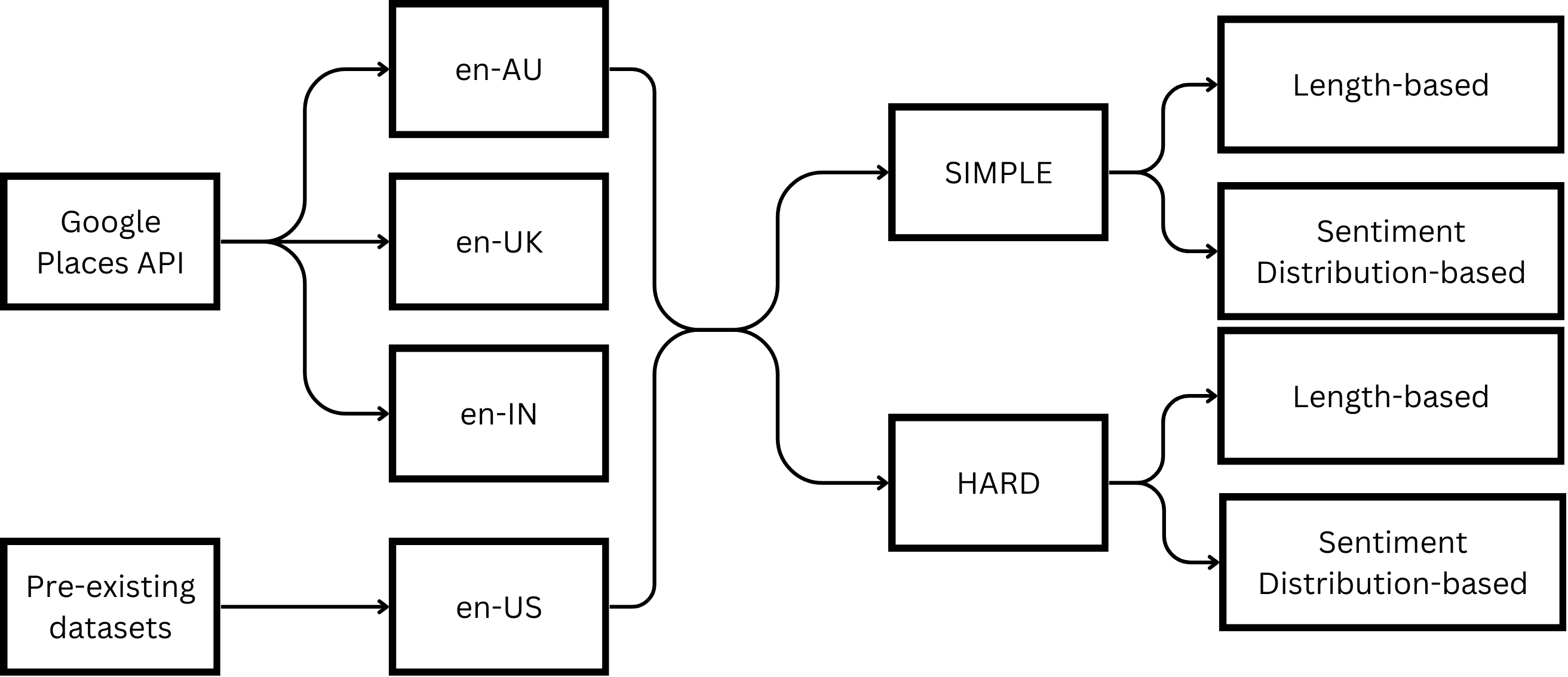
To address this question, we curate reviews from three locales - Austalian English (en-AU), Indian English (en-IN) and British English (en-UK), and use an existing dataset of reviews from Standard American English (en-US), as shown in Figure 1. By applying various data sampling techniques, we show the curation of an effective, challenging benchmark dataset, and present insights from a comprehensive evaluation of model performance on this dialectal data.
2 Related Work
The creation of benchmarks that reflect linguistic diversity is crucial for ensuring that language technologies are equitable and do not perpetuate biases against specific linguistic subgroups blodgett-etal-2020-language. Despite these efforts, language models often struggle with tasks involving dialects other than standard US-English, highlighting a significant gap in current evaluation practices joshi2024naturallanguageprocessingdialects; faisal2024dialectbench.
Traditional sentiment benchmarks like the Stanford Sentiment Treebank (SST-2) socher-etal-2013-recursive and the IMDB reviews dataset maas-etal-2011-learning focus on standard language forms and do not account for dialectal variations, limiting their applicability in multi-dialectal settings. Modern benchmarks such as GLUE DBLP:journals/corr/abs-1804-07461 and SuperGLUE DBLP:journals/corr/abs-1905-00537 aim for broader language understanding but still fall short in evaluating dialectal diversity.
A few datasets exist for dialectal sentiment analysis. SANA abdul-mageed-diab-2014-sana provides a multi-genre, multi-dialectal Arabic lexical dataset with over entries labeled for sentiment. A study on Tunisian Dialect Arabic medhaffar-etal-2017-sentiment introduces a -comment Facebook corpus, showing improved model performance on dialectal data compared to Modern Standard Arabic. Similarly, ArSAS d3cb00d902eb44a0a0d01b794e862787 offers a -tweet corpus over multiple dialects of Arabic annotated for speech-act recognition and sentiment, supporting research in both areas. boujou2021openaccessnlpdataset present a comprehensive dataset of over tweets in multiple Arabic dialects, labeled for dialect detection, topic detection, and sentiment analysis. In contrast, while there are robust resources for Arabic dialects, comparable datasets for English dialects remain limited.
Work in muhammad2023afrisentitwittersentimentanalysis advances dialectal benchmarks by providing a resource with tweet data annotated by native speakers for African languages and dialects, addressing gaps in existing benchmarked datasets. Similarly, fsih-etal-2022-benchmarking evaluate several Arabic language models against standard benchmarks for sentiment analysis, where it is shown that models trained on dialectal Arabic outperform general models, highlighting the need for benchmarks that reflect dialectal diversity.
3 Methodology
In this section, we detail the methodology employed to investigate the impact of linguistic variety on task performance. Our approach includes the collection and pre-processing of a diverse dataset of reviews from multiple locales using the Google Places API. We describe our criteria for selecting cities across Australia, India, and the United Kingdom, and include reviews from New York City to establish a baseline for Standard American English. Finally, we elaborate on our design choices focusing on label proximity, lexical properties, and semantic content to assess their influence on the task performances.
3.1 Dataset
We collect reviews and their corresponding ratings using the Google Places API111https://developers.google.com/maps/documentation/places/web-service/overview; Accessed on 23 July 2024 from the place types, also defined by the API. We do not collect or store information about the reviewer or the place to ensure the anonymity of the reviews. We process reviews by removing special characters, emoticons etc., to maintain uniform textual format.
3.2 Linguistic Variety
We gather reviews from cities across three different locales: Australia (en-AU), India (en-IN), and the United Kingdom (en-UK). The criteria for city selection are based on population thresholds specific to each country. In Australia, a city is defined as an urban center with a population of 10,000 persons or more222Australian Bureau of Statistics. https://www.abs.gov.au/statistics/standards; Accessed on 29 July 2024. For India, a city corresponds to a town with a population of 100,000 persons or more333Census India. http://www.censusindia.gov.in/Metadata/Metada.htm#2c; Accessed on 29 July 2024. In the United Kingdom, due to the complex nature of defining a city, we select geographic locations with populations exceeding 50,000 persons. We also utilize Google Places reviews from New York City li-etal-2022-uctopic; 10.1145/3539618.3592036, to establish a baseline for Standard American English (en-US). Finally, we filter out any non-English text using language probabilities calculated by fastText grave2018learning word vectors.
Locale 1 ★ 2 ★ 3 ★ 4 ★ 5 ★ en-US 5351 2389 1612 5142 15097 0.985 en-AU 924 359 510 1108 4570 0.998 en-UK 2691 955 1495 3399 13430 0.999 en-IN 4268 1306 3309 7127 15629 0.988
3.3 Design Choices
We employ several design choices to investigate their impact on task performance, focusing on label proximity, lexical properties, and semantic content.
Label-proximity
To explore the effect of target label proximity, we compare task performances on subsets with well-separated labels (1★and 5★; simple) and the subsets with closer labels (2★and 4★; hard).
Sampling based on review length
We examine the influence of review length by performing lexical splits based on word counts. Given a set of all words in a review (), each subset is sampled as follows:
-
•
len-75: Reviews with lengths greater than the first quartile.
-
•
len-50: Reviews with lengths greater than the median.
-
•
len-25: Reviews with lengths greater than the third quartile.
Sampling based on sentiment density
Given two sets of sentiment-bearing words (pos and neg), we compute the sentiment density in a review () as shown below: \linenomathAMS
Here calculates the number of words in a set. We then sample each subset as follows:
-
•
sent-75: Reviews with sentiment density greater than the first quartile.
-
•
sent-50: Reviews with sentiment density greater than the median.
-
•
sent-25: Reviews with sentiment density greater than the third quartile.
What is simple-len-75
4 Experiment Setup
We experiment with three encoder models namely, BERT (bert) devlin-etal-2019-bert, DistilBERT (distil) sanh2020distilbertdistilledversionbert, RoBERTa (roberta) zhuang-etal-2021-robustly. Given a variety, we perform ‘in-sample’ fine-tuning on all models for 10 epochs with early stopping, using Adam optimiser. All experiments are performed using 6 NVIDIA V100 GPUs, with a single seed for reproducibility. The statistics of each sample in each variety are reported in Table 3. We report our task performances on three macro-averaged metrics: precision (P), recall (R), and f1-score (F).
5 Evaluation
Locale simple hard P R F P R F en-US 92.7 94.3 93.5 85.5 88.0 86.5 \hdashline en-AU 96.2 98.4 97.2 82.4 83.1 81.8 en-UK 96.7 97.1 96.9 81.7 89.3 84.2 en-IN 95.0 95.1 95.0 77.5 74.4 75.6 \hdashline 95.2 96.3 95.7 81.8 83.7 82.0 (13.7)


Our evaluation of design choices addresses three questions: (a) What is the impact of label proximity on task performance?; (b) What is the impact of introducing dialectal text on task performance; (c) How to sample each subset of text to make the task more challenging for all models?
Table 4 shows the comparison of the average performance of models on reviews from each locale. The highest performance on the task is reported by models fine-tuned on en-AU (simple) with the F1-Score of 97.2. The worst performance is reported by the baseline models, with the average F1-Score of 93.5. Models report a degraded performance across reviews from all locales when the labels are changed from simple to hard, with an average decrease in the F1-score of 13.7. The idea of changing labels based on proximity has been explored earlier, and our results validate these claims. We further evaluate the impact of sampling on task performances.
5.1 Comparison on samples based on review length
Figure 2 shows the trend in average F1-score across all models when fine-tuned on various lexicon-based sampled subsets of reviews from each locale. Models trained on simple-len-75 sample of en-AU reviews, outperform other models, yielding an average F1-score of 98.3. The worst task performance was reported by models trained on hard-len-25 sample of en-IN reviews, yielding an average F1-score of 81.5. Our evaluation of lexicon-based sampling shows that models trained on very long reviews (*-len-25) yield higher task performances in most cases.
5.2 Comparison on samples based on sentiment density
Figure 2 shows the trend in average F1-score across all models when fine-tuned on various semantic-based sampled subsets of reviews from each locale. Models trained on simple-sent-75 sample of en-AU reviews, outperform other models, yielding an average F1-score of 97.2. This performance degrades as the polarity density in the sample increases, with the worst F1-score of 64.8 for models trained on hard-sent-25. Our evaluation of semantic-based sampling shows that models trained on reviews with higher polarity density (*-sent-25) yield degraded task performances in most cases.
5.3 Impact of linguistic variety
The models trained on the simple-len-* samples from en-IN, match or sometimes outperform the models trained on the same samples from inner-circle varieties. But the performances improve for models trained on the hard-len-* samples from inner-circle varieties, while they degrade on en-IN samples. This disparity in performances based on linguistic variety is also seen in models trained on simple-sent-* samples. However, the semantic-based sampling yields the opposite effect on inner-circle varieties as the sentiment density increases in hard samples.
6 Conclusion & Future Work
This paper focused on evaluating the impact of the linguistic variety and various data-related strategies that make sentiment classification on Google Places reviews challenging for large language models. To introduce linguistic variety, we collected reviews from three locales– Australia, India, and the UK. We also utilised the existing dataset of reviews from New York for the baseline. The strategies included changing target labels and data sampling based on length and sentiment density.
Our results show that models reported higher performance on subsets with well-separated labels (simple) compared to those with closer labels (hard). This validates the idea that label proximity impacts model performance on the task, motivating the need for fine-grained analysis in sentiment classification tasks. Our evaluation of data sampling strategies showed that models trained on longer reviews (*-len-25) generally outperformed those trained on shorter ones. This suggests that longer texts provide more contextual information, enabling models to make more accurate sentiment predictions. However, models performed worse on reviews with higher sentiment density (*-sent-25), especially when trained on subsets with hard labels. This indicates that higher sentiment density can introduce ambiguity, leading to degradation in model performances on the task. Models trained on inner-circle English varieties (en-US, en-AU, en-UK) generally outperformed those trained on en-IN, particularly in more challenging tasks (hard labels and samples with long review lengths). These findings from our evaluation highlight the need for incorporating diverse linguistic varieties along with better sampling strategies while creating benchmarks to better reflect real-world complexities.
7 Limitations
8 Ethics Statement
Appendix A Data statistics for each sample
| Length | |||||
|---|---|---|---|---|---|
| Locale | Quartiles | Rating | |||
| 1 ★ | 5 ★ | 2 ★ | 4 ★ | ||
| en-US | 25% | 788 | 4096 | 363 | 1326 |
| 25-50% | 752 | 3736 | 405 | 1311 | |
| 50-75% | 1265 | 3854 | 660 | 1342 | |
| 75% | 2373 | 2547 | 884 | 953 | |
| \hdashlineen-AU | 25% | 95 | 1282 | 49 | 263 |
| 25-50% | 175 | 1225 | 71 | 257 | |
| 50-75% | 276 | 1149 | 92 | 273 | |
| 75% | 378 | 914 | 147 | 315 | |
| \hdashlineen-UK | 25% | 315 | 3870 | 113 | 746 |
| 25-50% | 506 | 3482 | 174 | 801 | |
| 50-75% | 726 | 3397 | 263 | 935 | |
| 75% | 1144 | 2681 | 405 | 917 | |
| \hdashlineen-IN | 25% | 593 | 4726 | 225 | 1451 |
| 25-50% | 881 | 3975 | 253 | 1730 | |
| 50-75% | 1322 | 3711 | 363 | 1911 | |
| 75% | 1472 | 3217 | 465 | 2035 | |
| Polarity Difference | |||||
| Locale | Quartiles | Rating | |||
| 1 ★ | 5 ★ | 2 ★ | 4 ★ | ||
| en-US | 25% | 2110 | 238 | 638 | 201 |
| 25-50% | 1465 | 1316 | 587 | 624 | |
| 50-75% | 1164 | 7983 | 758 | 2687 | |
| 75% | 439 | 4696 | 329 | 1420 | |
| \hdashlineen-AU | 25% | 698 | 430 | 200 | 197 |
| 25-50% | 150 | 1127 | 89 | 270 | |
| 50-75% | 49 | 1233 | 37 | 295 | |
| 75% | 27 | 1780 | 33 | 346 | |
| \hdashlineen-UK | 25% | 2049 | 1051 | 573 | 573 |
| 25-50% | 419 | 2791 | 92 | 783 | |
| 50-75% | 173 | 4983 | 121 | 1141 | |
| 75% | 50 | 4605 | 69 | 902 | |
| \hdashlineen-IN | 25% | 2783 | 1342 | 533 | 879 |
| 25-50% | 677 | 3541 | 296 | 1563 | |
| 50-75% | 589 | 5473 | 323 | 2366 | |
| 75% | 219 | 5273 | 154 | 2319 | |
Appendix B Simple v Hard labels
Locale Split bert distil roberta P R F P R F P R F P R F en-US simple 93.3 94.9 94.1 92.6 95.2 93.8 92.2 92.8 92.5 92.7 94.3 93.5 hard 85.4 87.4 86.3 83.0 86.0 84.0 88.1 90.6 89.1 85.5 88.0 86.5 \hdashline en-AU simple 92.7 98.2 95.2 97.0 97.8 97.4 98.8 99.2 99.0 96.2 98.4 97.2 hard 81.0 73.7 76.2 78.1 85.0 79.9 88.1 90.8 89.4 82.4 83.1 81.8 \hdashline en-UK simple 96.0 97.9 97.0 96.9 95.5 96.2 97.1 97.8 97.5 96.7 97.1 96.9 hard 82.8 88.7 85.1 79.5 88.7 81.9 82.8 90.6 85.5 81.7 89.3 84.2 \hdashline en-IN simple 97.3 95.5 96.4 95.4 94.3 94.9 92.2 95.6 93.8 95.0 95.1 95.0 hard 77.1 73.5 75.1 75.4 77.4 76.3 79.9 72.4 75.3 77.5 74.4 75.6
Appendix C Length based splits
simple Locale Bin bert distil roberta P R F P R F P R F P R F en-US 25% 93.0 94.4 93.7 94.5 94.8 94.6 91.9 95.1 93.3 93.1 94.8 93.9 50% 97.5 96.8 97.2 94.5 95.5 95.0 96.1 96.9 96.5 96.0 96.4 96.2 75% 97.0 97.0 97.0 96.4 96.3 96.3 97.0 97.0 97.0 96.8 96.8 96.8 \hdashline en-AU 25% 98.5 98.5 98.5 97.7 99.4 98.5 97.7 99.4 98.5 98.0 99.1 98.5 50% 96.8 98.2 97.5 97.4 96.4 96.9 96.1 98.0 97.0 96.8 97.5 97.1 75% 98.1 98.1 98.1 96.2 96.2 96.2 98.7 99.4 99.1 97.7 97.9 97.8 \hdashline en-UK 25% 95.3 98.3 96.7 95.9 97.8 96.8 95.7 98.3 97.0 95.6 98.1 96.8 50% 97.2 98.6 97.9 97.9 98.6 98.2 97.8 99.1 98.4 97.6 98.8 98.1 75% 97.2 97.7 97.5 95.4 96.5 96.0 97.5 97.5 97.5 96.7 97.2 97.0 \hdashline en-IN 25% 96.8 97.5 97.1 95.1 95.3 95.2 96.5 95.5 96.0 96.1 96.1 96.1 50% 97.2 97.9 97.6 96.5 97.0 96.8 97.0 98.0 97.4 96.9 97.6 97.2 75% 97.6 98.9 98.2 97.6 97.8 97.7 99.1 98.8 99.0 98.1 98.5 98.3 hard Locale Bin bert distil roberta P R F P R F P R F P R F en-US 25% 86.4 88.5 87.2 82.3 85.1 82.8 87.2 89.3 88.5 85.3 87.6 86.2 50% 85.0 86.2 85.2 86.4 85.9 86.1 90.2 90.4 90.3 87.2 87.5 87.2 75% 89.7 89.6 89.7 87.5 86.7 86.4 88.9 91.6 90.7 88.7 89.3 88.9 \hdashline en-AU 25% 87.2 89.3 88.1 88.0 84.7 86.1 87.2 89.3 88.1 87.5 87.8 87.6 50% 81.4 78.9 80.0 80.9 80.1 80.5 85.8 84.0 84.8 82.7 81.0 81.8 75% 88.9 91.6 90.0 86.4 90.0 87.6 88.9 91.6 90.0 88.1 91.1 89.2 \hdashline en-UK 50% 82.1 89.5 84.4 83.7 86.4 84.9 82.3 88.9 84.5 82.7 88.3 84.6 50% 81.4 87.2 83.1 84.7 77.3 79.9 83.9 84.2 84.1 83.3 82.9 82.4 75% 92.0 94.2 93.0 90.1 93.1 91.3 96.4 96.4 96.4 92.8 94.6 93.6 \hdashline en-IN 25% 78.4 83.1 80.4 80.0 82.5 81.2 83.7 76.5 79.4 80.7 80.7 80.3 50% 85.2 82.4 83.7 76.9 83.2 79.3 87.8 86.3 87.0 83.3 84.0 83.3 75% 81.5 87.4 83.8 82.1 77.5 79.5 81.4 89.1 84.3 81.7 84.7 82.5
Appendix D Polarity based splits
simple Locale Bin bert distil roberta P R F P R F P R F P R F en-US 25% 90.3 95.7 92.4 91.7 92.3 92.0 91.2 95.5 93.1 91.1 94.5 92.5 50% 84.5 94.6 88.6 89.9 92.2 91.0 89.6 96.3 92.6 88.0 94.4 90.7 75% 88.4 95.3 91.5 96.7 91.8 94.1 96.3 96.3 96.3 93.8 94.5 94.0 \hdashline en-AU 25% 90.1 95.0 92.4 85.3 92.5 88.5 87.9 86.4 87.1 87.8 91.3 89.3 50% 99.8 93.8 96.6 99.5 81.3 88.2 88.7 93.4 90.9 96.0 89.5 91.9 75% 68.7 98.6 76.5 100.0 100.0 100.0 49.2 50.0 49.6 72.6 82.8 75.3 \hdashline en-UK 25% 94.2 98.1 96.1 97.5 89.0 92.8 91.2 94.8 92.9 94.3 94.0 94.0 50% 88.3 86.7 87.5 89.6 84.6 86.9 48.8 50.0 49.4 75.6 73.8 74.6 75% 99.9 90.0 94.4 74.9 89.6 80.5 49.4 50.0 49.7 74.7 76.5 74.8 \hdashline en-IN 25% 88.8 93.4 91.0 89.7 93.5 91.5 90.3 93.9 92.0 89.6 93.6 91.5 50% 93.0 90.8 91.6 92.2 92.7 92.4 87.3 92.8 89.8 90.8 92.1 91.3 75% 86.3 92.5 89.1 94.2 88.4 91.1 86.8 94.8 90.4 89.1 91.9 90.2 hard Locale Bin bert distil roberta P R F P R F P R F P R F en-US 25% 82.6 86.9 84.2 82.5 86.3 84.0 88.5 85.5 86.8 84.5 86.2 85.0 50% 81.6 86.5 83.6 80.9 86.1 83.0 80.4 85.2 82.3 80.9 85.9 83.0 75% 89.4 90.3 89.8 85.5 81.2 83.1 88.4 92.6 90.3 87.8 88.0 87.7 \hdashline en-AU 25% 84.0 82.2 83.0 79.1 72.8 75.3 78.1 96.4 84.1 80.4 83.8 80.8 50% 45.1 50.0 47.4 87.7 77.8 81.8 45.1 50.0 47.4 59.3 59.3 58.9 75% 80.5 73.5 76.4 97.2 75.0 81.9 97.2 75.0 81.9 91.6 74.5 80.1 \hdashline en-UK 50% 76.9 87.7 80.9 79.5 81.5 80.5 44.1 50.0 46.9 66.8 73.1 69.4 50% 70.2 88.9 75.0 73.2 78.6 75.6 84.0 90.4 86.8 75.8 86.0 79.1 75% 97.9 71.4 78.9 97.4 64.3 70.9 90.6 85.1 87.6 95.3 73.6 79.1 \hdashline en-IN 25% 67.1 81.3 70.1 82.1 78.4 80.1 70.6 85.4 74.5 73.3 81.7 74.9 50% 67.2 77.9 70.5 82.2 70.9 75.0 45.4 50.0 47.5 64.9 66.3 64.3 75% 80.7 86.0 83.1 83.4 65.2 70.4 46.7 50.0 48.3 70.3 67.1 67.3