This paper was converted on www.awesomepapers.org from LaTeX by an anonymous user.
Want to know more? Visit the Converter page.

Mittag-Leffler stability of complete monotonicity-preserving schemes for time-dependent coefficients sub-diffusion equations

Wen Dong [email protected] Dongling Wang [email protected], ORCID:0000-0001-8509-2837 School of Mathematics, Northwest University, Xi’an, Shaanxi, 710127, P.R. China School of Mathematics and Computational Science, Xiangtan University, Xiangtan, Hunan 411105, China
Abstract

A key characteristic of the anomalous sub-solution equation is that the solution exhibits algebraic decay rate over long time intervals, which is often refered to the Mittag-Leffler type stability. For a class of power nonlinear sub-diffusion models with variable coefficients, we prove that their solutions have Mittag-Leffler stability when the source functions satisfy natural decay assumptions. That is the solutions have the decay rate u(t)Ls(Ω)=O(t(α+β)/γ)\|u(t)\|_{L^{s}(\Omega)}=O\left(t^{-(\alpha+\beta)/\gamma}\right) as tt\rightarrow\infty, where α\alpha, γ\gamma are positive constants, β(α,)\beta\in(-\alpha,\infty) and s(1,)s\in(1,\infty). Then we develop the structure preserving algorithm for this type of model. For the complete monotonicity-preserving (𝒞\mathcal{CM}-preserving) schemes developed by Li and Wang (Commun. Math. Sci., 19(5):1301-1336, 2021), we prove that they satisfy the discrete comparison principle for time fractional differential equations with variable coefficients. Then, by carefully constructing the fine the discrete supersolution and subsolution, we obtain the long time optimal decay rate of the numerical solution unLs(Ω)=O(tn(α+β)/γ)\|u_{n}\|_{L^{s}(\Omega)}=O\left(t_{n}^{-(\alpha+\beta)/\gamma}\right) as tnt_{n}\rightarrow\infty, which is fully agree with the theoretical solution. Finally, we validated the analysis results through numerical experiments.

keywords:
time-dependent coefficient sub-diffusion equations, 𝒞\mathcal{CM}-preserving schemes, Mittag-Leffler type stability, discrete comparison principle.
journal: XXXlabel1label1footnotetext: The research of Dongling Wang is supported in part by NSFC (No. 12271463) and Outstanding Youth Foundation of Department of Education in Hunan Province (No. 22B0173).
Declarations of interest: none.

1 Introduction

A typical application of time fractional equations is to describe various anomalous diffusion models, namely sub-diffusion and super-diffusion phenomena. For the standard diffusion process, which is usually described by the classical heat equation, where the mean square displacement (MSD) of particles is a linear function of time, i.e., x2(t)Ct\langle x^{2}(t)\rangle\sim Ct. 111As usual, our notation \sim here represents the asymptotic limit limtx2(t)t=C\lim_{t\to\infty}\frac{\langle x^{2}(t)\rangle}{t}=C, where CC represents a general positive constant, which may take different values in different places, but is always independent of tt or nn. We also use the standard notation OO to represent a certain asymptotic order, for example y(t)=O(tα)y(t)=O(t^{-\alpha}) means limt|y(t)tα|C\lim_{t\to\infty}\left|\frac{y(t)}{t^{-\alpha}}\right|\leq C. However, many actual model data indicate that the MSD of anomalous diffusion processes may have a form x2(t)Ctα\langle x^{2}(t)\rangle\sim Ct^{\alpha}, where α(0,2)\alpha\in(0,2). Based on random walk theory, we can rigorously derive fractional diffusion equations, where Caputo derivatives are typically used in the time direction instead of classical first-order derivatives [3, 8]. Specifically, when α(0,1)\alpha\in(0,1), it is referred to as the sub-diffusion process.

For the time fractional order model, its solutions exhibit asymptotic behavior completely different from the standard diffusion equation over a long time interval. In fact, solutions to time fractional equations typically have algebraic decay rates, while standard first-order equations have exponential decay rates. This can be seen from the simple example below. Consider the fractional ODE: Dtαy(t)=λy(t)D_{t}^{\alpha}y(t)=\lambda y(t) with y(0)=y0>0y(0)=y_{0}>0, where the Caputo fractional derivative of order α\alpha is defined by Dtαy(t):=1Γ(1α)0t(ts)αy(s)𝑑sD_{t}^{\alpha}y(t):=\frac{1}{\Gamma(1-\alpha)}\int_{0}^{t}(t-s)^{-\alpha}y^{\prime}(s)ds [8]. The solution is given by y(t)=y0Eα,1(λtα)y(t)=y_{0}E_{\alpha,1}(\lambda t^{\alpha}), where Eα,β(t)E_{\alpha,\beta}(t) is the Mittag-Leffler funciton. When λ<0\lambda<0, we have y(t)Ctαy(t)\sim Ct^{-\alpha} by the asymptotic expansion formula of Mittag-Leffler funciton. This long-term algebraic decay rate is commonly referred to as Mittag-Leffler stability. Another surprising result is presented in [19], which shows that for the fractional ODE: Dtαy(t)=λyγ(t)D_{t}^{\alpha}y(t)=\lambda y^{\gamma}(t) with y0>0,γ>0y_{0}>0,\gamma>0 and λ<0\lambda<0, the solution has the asymptotic decay rate y(t)Ctαγy(t)\sim Ct^{-\frac{\alpha}{\gamma}}.

Once we have the above two results and combine appropriate energy methods, we can obtain the long-term decay rate estimation of the standard Ls(Ω)L^{s}(\Omega)-norm (s>1)(s>1) for the solution of linear or some nonlinear anomalous diffusion model. See for example [4, 10, 19, 2]. Currently, most of these analyses are focused on constant coefficient equations. However, the anomalous diffusion problems can be both constant coefficients and variable coefficients. Compared with constant coefficient equations, the variable coefficient equations are appropriate for modeling of anomalous diffusive processes in turbulent media. For instance, modeling sub-diffusive transport inside a fractured porous media [6]. Diffusion representation of tracer particles in heterogeneous biological ambient fluids [1]. In particular, the application of the time dependence coefficient is a new perspective of coupling the spatial and temporal variables, which avoids the divergence caused by the long tail of the temporal probability distribution at a fixed time [5]. For more information on the application of variable coefficients to more complex physical and biological systems, see also [3, 5, 7].

The aim of this paper is to study both theoretically and numerically the long time Mittag-Leffler stability of the solutions for a class of nonlinear anomalous diffusion models with time-dependent coefficients

{Dtαu(t,x)+νtβ𝒩(u(t,x))=f(t,x)fort>0,xΩ,u(0,x)=u0(x)0forxΩ,u(t,x)=0fort>0,xΩ,\left\{\begin{aligned} &D_{t}^{\alpha}u(t,x)+\nu t^{\beta}\mathcal{N}(u(t,x))=f(t,x)~{}~{}for~{}t>0,~{}x\in\Omega,\\ &u(0,x)=u_{0}(x)\geq 0~{}~{}for~{}x\in\Omega,\\ &u(t,x)=0~{}~{}~{}for~{}t>0,~{}x\in\partial\Omega,\end{aligned}\right. (1)

where 0<α<10<\alpha<1, β>α\beta>-\alpha, ν>0\nu>0, and Ωd(d1)\Omega\subset\mathbb{R}^{d}~{}(d\geq 1) is a bounded domain with smooth boundary Ω\partial\Omega. And 𝒩(u)\mathcal{N}(u) can be linear or nonlinear operator, some typical examples including the Laplace operator 𝒩(u)=Δu\mathcal{N}(u)=-\Delta u; the pp-Laplace operator 𝒩(u)=Δpu\mathcal{N}(u)=-\Delta_{p}u with Δpu=div(|u|p2u)\Delta_{p}u=\mathrm{div}(|\nabla u|^{p-2}\nabla u) and the mean curvature operator 𝒩(u)=div(u1+|u|2)\mathcal{N}(u)=-\mathrm{div}\Big{(}\frac{\nabla u}{\sqrt{1+|\nabla u|^{2}}}\Big{)}. Following [4, 16],we assume that 𝒩(u)\mathcal{N}(u) satisfies the following structural assumption

w(t,)Ls(Ω)s1+γCNΩws1(t,x)𝒩(w(t,x))𝑑x for wLs(Ω),\|w(t,\cdot)\|_{L^{s}(\Omega)}^{s-1+\gamma}\leq C_{N}\int_{\Omega}w^{s-1}(t,x)\mathcal{N}(w(t,x))dx~{}\text{ for }~{}w\in L^{s}(\Omega), (2)

where s(1,)s\in(1,\infty), γ(0,+)\gamma\in(0,+\infty) and CN>0C_{N}>0. One can verify that the above example of 𝒩(u)\mathcal{N}(u) indeed satisfies the elliptical structure assumption [4, 14]. The non-zero source terms f(t,x)f(t,x) and satisfies the decay estimate

f(t)Ls(Ω)Ktβ(t+1)α+βt>0,s(1,),K>0.\|f(t)\|_{L^{s}(\Omega)}\leq\frac{Kt^{\beta}}{(t+1)^{\alpha+\beta}}~{}~{}\forall t>0,~{}\forall s\in(1,\infty),~{}K>0. (3)

Let uu be the solution of (1). Under the above assumptions, we can establish the long-term estimation of u(t,)Ls(Ω)\|u(t,\cdot)\|_{L^{s}(\Omega)}, i.e. Mittag-Leffler stability, by combining the energy method with the long-term estimation of time fractional ODEs. For the homogeneous linear constant coefficient equation with β=0,f=0\beta=0,f=0 and 𝒩(u)=Δu\mathcal{N}(u)=-\Delta u, we can apply standard eigenvalue and eigenfunction pairs methods to obtain that u(t,)Ls(Ω)Ctα\|u(t,\cdot)\|_{L^{s}(\Omega)}\sim Ct^{-\alpha}. For the constant coefficient nonlinear equation with β=0\beta=0 and 𝒩(u)\mathcal{N}(u) satisfying (2), it is shown that u(t,)Ls(Ω)Ctα/γ\|u(t,\cdot)\|_{L^{s}(\Omega)}\sim Ct^{-\alpha/\gamma}; see [16, 4, 2]. And for the homogeneous varying coefficient nonlinear equation with f=0f=0 and 𝒩(u)\mathcal{N}(u) satisfying (2), the asymptotic estimate u(t,)Ls(Ω)Ct(α+β)/γ\|u(t,\cdot)\|_{L^{s}(\Omega)}\sim Ct^{-(\alpha+\beta)/\gamma} for weak solution is obtained in [14], from which can see from that the time-dependent factor tβt^{\beta} has a direct impact on the long-term decay rate of the solution.

At present, most numerical methods for time fractional equations focus on the reduction in numerical convergence rate caused by weak singularity of the solution near the initial moment. Various effective techniques have been developed to restore high-order convergence of numerical methods; see [13, 11, 15, 9]. From the perspective of the structure-preserving algorithm, we naturally hope that the numerical solution can preserve the long-term optimal decay rate of the sub-diffusion equation, that is, establish numerical Mittag-Leffler stability. At present, there are relatively few research results on qualitative analysis of numerical solutions to anomalous diffusion equations, especially long-term behavior analysis. For the linear time fractional evolutional equation, the numerical ML stability, i.e. unLs(Ω)Ctnα\|u_{n}\|_{L^{s}(\Omega)}\sim Ct_{n}^{-\alpha} is established in [18] through singularity analysis of the generating function of the numerical solution, where unu_{n} is the numerical approximation of uu at tnt_{n}. For the constant coefficient nonlinear equation with β=0\beta=0 and 𝒩(u)\mathcal{N}(u) satisfying (2), the numerical ML stability as unLs(Ω)Ctnα/γ\|u_{n}\|_{L^{s}(\Omega)}\sim Ct_{n}^{-\alpha/\gamma} was recently established in [17], using the discrete comparison principle and the method of constructing fine discrete sup and sub solutions. The key to success here lies in a class of time fractional derivative structure-preserving discrete schemes, namely the 𝒞\mathcal{CM}-preserving schemes developed in [12]. The discrete coefficients of this type of numerical method have many excellent properties.

The objective of this article is twofold.

  • 1.

    We derive the long-term decay estimate for the solution of the general non-homogeneous variable coefficient nonlinear equation (1) with β0,f0\beta\neq 0,f\neq 0 and 𝒩(u)\mathcal{N}(u) satisfying (2) and prove that u(t,)Ls(Ω)Ct(α+β)/γ\|u(t,\cdot)\|_{L^{s}(\Omega)}\sim Ct^{-(\alpha+\beta)/\gamma}. Our results extend the work of [14, 2].

  • 2.

    We establish the numerical ML stability for (1) based on the 𝒞\mathcal{CM}-preserving schemes and show that unLs(Ω)Ctn(α+β)/γ\|u_{n}\|_{L^{s}(\Omega)}\sim Ct_{n}^{-(\alpha+\beta)/\gamma}. Firstly, we prove that the 𝒞\mathcal{CM}-preserving schemes also satisfies the discrete comparison principle for variable coefficient equations. Then, applying this result, we construct discrete sup and sub solutions with variable coefficients to obtain the expected optimal numerical decay rate estimate. Our work in this article extend the results in [17] from homogeneous constant coefficient equations to non-homogeneous, variable coefficient equations.

The rest of this article is organized as follows. In Section 2, we derive the long time decay rate of continuous solutions for (1) and provide detailed proofs of the estimates. In Section 3, we recall 𝒞\mathcal{CM}-preserving schemes on uniform mesh tn=nτt_{n}=n\tau with time step size τ>0\tau>0 and their main properties. In Section 4, we establish the discrete numerical ML stability for (1). We first derive the discrete comparison principle of 𝒞\mathcal{CM}-preserving schemes for a class of time-dependent fractional ODEs. Then, by constructing discrete sub and sup solution we show the numerical ML stability for fractional non-homogeneous, variable coefficient ODEs. Then, by establishing a variable coefficient discrete energy inequality, we obtain the estimate of the long-term decay rate of the numerical solution of (1). Finally, we present several typical numerical examples to illustrate and verify the optical numerical decay rate in Section 5.

2 Decay estimate for nonlinear models with time-dependent coefficients

Consider the time-dependent coefficients fractional ODE, which highlight the influence of tβt^{\beta}:

Dtαy(t)+νtβyγ(t)=0 with y(0)=y0>0,D_{t}^{\alpha}y(t)+\nu t^{\beta}y^{\gamma}(t)=0\text{ with }y(0)=y_{0}>0, (4)

where 0<α<10<\alpha<1, β>α\beta>-\alpha, γ>0\gamma>0 and ν>0\nu>0. The decay result concerning (4) reads as follows.

Lemma 2.1.

[14] Let yC(+)y\in C(\mathbb{R}_{+}) be the solution of (4). Then there exist C1,C2>0C_{1},C_{2}>0 such that

C11+tα+βγy(t)C21+tα+βγfort0.\frac{C_{1}}{1+t^{\frac{\alpha+\beta}{\gamma}}}\leq y(t)\leq\frac{C_{2}}{1+t^{\frac{\alpha+\beta}{\gamma}}}~{}~{}for~{}t\geq 0. (5)

Note that when β=0\beta=0, the fractional ODE (4) is reduced to the power nonlinear equation and its solution has decay rate y(t)Ctα/γy(t)\sim Ct^{-\alpha/\gamma} [16]. Further, when β=0\beta=0 and γ=1\gamma=1, it becomes fractional linear ODE and the solution has the decay rate y(t)tαy(t)\sim t^{-\alpha}. Our first result below is to extend the estimation of the long-term decay rate of homogeneous equation (4) to non-homogeneous cases with source terms.

The proof the Mittag-Leffler stability of fractional ODEs in [16, 14] is mainly based on the comparison principle and the construction of appropriate barrier functions.

Lemma 2.2 (Fractional comparison principle).

[16] Let T>0T>0 and gC()g\in C(\mathbb{R}). Assume that gg is nondecreasing. Suppose that uu, wH11([0,T])w\in H_{1}^{1}([0,T]) satisfy u(0)w(0)u(0)\leq w(0) and

Dtα(uu(0))+g(u)\displaystyle D_{t}^{\alpha}(u-u(0))+g(u) 0,a.a.t(0,T),\displaystyle\leq 0,~{}a.a.~{}t\in(0,T),
Dtα(ww(0))+g(w)\displaystyle D_{t}^{\alpha}(w-w(0))+g(w) 0,a.a.t(0,T).\displaystyle\geq 0,~{}a.a.~{}t\in(0,T).

Then u(t)w(t)u(t)\leq w(t) for all t[0,T]t\in[0,T].

It is noted that in (4), the nonlinear function g(y):=νtβyγg(y):=\nu t^{\beta}y^{\gamma} is positive and nondecreasing, which allows the utilization of Lemma 2.2 to prove Lemma 2.1. Now we extend Lemma 2.1 to non-homogeneous cases with source terms.

Theorem 2.1.

Consider the fractional ODE: Dtαφ(t)+νtβφγ(t)=f(t)D_{t}^{\alpha}\varphi(t)+\nu t^{\beta}\varphi^{\gamma}(t)=f(t) with φ(0)=φ0>0\varphi(0)=\varphi_{0}>0 and assume that ff satisfies |f|<Ktβ/(t+1)α+β|f|<Kt^{\beta}/(t+1)^{\alpha+\beta} for some K>0K>0. Then there exists constants C˘1\breve{C}_{1}, C˘2>0\breve{C}_{2}>0 such that the solution φ\varphi satisfies

C˘11+tα+βγφ(t)C˘21+tα+βγfort0.\frac{\breve{C}_{1}}{1+t^{\frac{\alpha+\beta}{\gamma}}}\leq\varphi(t)\leq\frac{\breve{C}_{2}}{1+t^{\frac{\alpha+\beta}{\gamma}}}~{}~{}for~{}t\geq 0. (6)

Our main idea of proof is as follows: by constructing new fine upper and lower solutions, we can control the source function ff and obtain inequality of the corresponding homogeneous equation, which can be applied to Lemma 2.2.

Proof.

By the assumption |f|<Ktβ/(t+1)α+β|f|<Kt^{\beta}/(t+1)^{\alpha+\beta}, we have

Ktβ(t+1)α+βDtαφ(t)+νtβφγ(t)Ktβ(t+1)α+β.\frac{-Kt^{\beta}}{(t+1)^{\alpha+\beta}}\leq D_{t}^{\alpha}\varphi(t)+\nu t^{\beta}\varphi^{\gamma}(t)\leq\frac{Kt^{\beta}}{(t+1)^{\alpha+\beta}}. (7)

Define φ0γ=max{K/ν,(4νΓ(1α))γ/(1γ)}\varphi_{0}^{\gamma}=\max\left\{K/\nu,(4\nu\Gamma(1-\alpha))^{\gamma/(1-\gamma)}\right\}.

I. Construct a subsolution. Consider the function

u(t)={φ02νφ0γΓ(1+β)Γ(1+α+β)tα+βfort[0,ϵ],Cφ0ϵα+βγtα+βγfort>ϵ,u(t)=\left\{\begin{aligned} &\varphi_{0}-\frac{2\nu\varphi_{0}^{\gamma}\Gamma(1+\beta)}{\Gamma(1+\alpha+\beta)}t^{\alpha+\beta}~{}~{}for~{}t\in[0,\epsilon],\\ &C_{*}\varphi_{0}\epsilon^{\frac{\alpha+\beta}{\gamma}}t^{-\frac{\alpha+\beta}{\gamma}}~{}~{}for~{}t>\epsilon,\end{aligned}\right. (8)

where

ϵ=((1C)φ01γΓ(1+α+β)2νΓ(1+β))1/(α+β),C=min{(Γ(1+β)Γ(1+α+β)Γ(1α))1γ,21}.\epsilon=\left(\frac{(1-C_{*})\varphi_{0}^{1-\gamma}\Gamma(1+\alpha+\beta)}{2\nu\Gamma(1+\beta)}\right)^{1/(\alpha+\beta)},~{}C_{*}=\min\left\{\left(\frac{\Gamma(1+\beta)}{\Gamma(1+\alpha+\beta)\Gamma(1-\alpha)}\right)^{\frac{1}{\gamma}},2^{-1}\right\}.

Using the definition of u(t)u(t), it is easy to find that vv is monotonically decreasing. Now we show that u(t)u(t) is a sub solution for φ\varphi over the interval [0,ϵ](ϵ,)[0,\epsilon]\cup(\epsilon,\infty). For t[0,ϵ]t\in[0,\epsilon], by noting φ0γK/ν\varphi_{0}^{\gamma}\geq K/\nu and ν,φ0>0\nu,~{}\varphi_{0}>0, we have

Dtαu(t)+νtβuγ(t)\displaystyle D_{t}^{\alpha}u(t)+\nu t^{\beta}u^{\gamma}(t) =2νtβφ0γ+νtβ(φ02νφ0γΓ(1+β)Γ(1+α+β)tα+β)γ\displaystyle=-2\nu t^{\beta}\varphi_{0}^{\gamma}+\nu t^{\beta}\left(\varphi_{0}-\frac{2\nu\varphi_{0}^{\gamma}\Gamma(1+\beta)}{\Gamma(1+\alpha+\beta)}t^{\alpha+\beta}\right)^{\gamma}
νtβφ0γtβKtβK(t+1)α+β.\displaystyle\leq-\nu t^{\beta}\varphi_{0}^{\gamma}\leq-t^{\beta}K\leq-\frac{t^{\beta}K}{(t+1)^{\alpha+\beta}}.

On the other hand, for t>ϵt>\epsilon we have v0v^{\prime}\leq 0. Therefor,

Dtαu(t)+νtβuγ(t)\displaystyle D_{t}^{\alpha}u(t)+\nu t^{\beta}u^{\gamma}(t) 1Γ(1α)0ϵ(ts)αv(s)𝑑s+νtβCγφ0γϵα+βt(α+β)\displaystyle\leq\frac{1}{\Gamma(1-\alpha)}\int_{0}^{\epsilon}(t-s)^{-\alpha}v^{\prime}(s)ds+\nu t^{\beta}C_{*}^{\gamma}\varphi_{0}^{\gamma}\epsilon^{\alpha+\beta}t^{-(\alpha+\beta)}
2νΓ(1+β)Γ(1+α+β)Γ(1α)φ0γtαϵα+β+νtαCγφ0γϵα+β\displaystyle\leq-\frac{2\nu\Gamma(1+\beta)}{\Gamma(1+\alpha+\beta)\Gamma(1-\alpha)}\varphi_{0}^{\gamma}t^{-\alpha}\epsilon^{\alpha+\beta}+\nu t^{-\alpha}C_{*}^{\gamma}\varphi_{0}^{\gamma}\epsilon^{\alpha+\beta}
=νtαφ0γϵα+β(2Γ(1+β)Γ(1+α+β)Γ(1α)Cγ).\displaystyle=-\nu t^{-\alpha}\varphi_{0}^{\gamma}\epsilon^{\alpha+\beta}\left(\frac{2\Gamma(1+\beta)}{\Gamma(1+\alpha+\beta)\Gamma(1-\alpha)}-C_{*}^{\gamma}\right).

By the definitions of ϵ\epsilon, CC_{*} and noting that φ0>[4νΓ(1α)]1/(1γ)\varphi_{0}>[4\nu\Gamma(1-\alpha)]^{1/(1-\gamma)}, we confirm that

ϵα+β(2Γ(1+β)Γ(1+α+β)Γ(1α)Cγ)ϵα+βΓ(1+β)Γ(1+α+β)Γ(1α)=(1C)φ01γ2νΓ(1α)φ01γ4νΓ(1α)1,\epsilon^{\alpha+\beta}\left(\frac{2\Gamma(1+\beta)}{\Gamma(1+\alpha+\beta)\Gamma(1-\alpha)}-C_{*}^{\gamma}\right)\geq\epsilon^{\alpha+\beta}\frac{\Gamma(1+\beta)}{\Gamma(1+\alpha+\beta)\Gamma(1-\alpha)}=\frac{(1-C_{*})\varphi_{0}^{1-\gamma}}{2\nu\Gamma(1-\alpha)}\geq\frac{\varphi_{0}^{1-\gamma}}{4\nu\Gamma(1-\alpha)}\geq 1,

then

Dtαu(t)+νtβuγ(t)νtαφ0γ=νtβt(α+β)φ0γtβK(t+1)α+β.D_{t}^{\alpha}u(t)+\nu t^{\beta}u^{\gamma}(t)\leq-\nu t^{-\alpha}\varphi_{0}^{\gamma}=-\nu t^{\beta}t^{-(\alpha+\beta)}\varphi_{0}^{\gamma}\leq-\frac{t^{\beta}K}{(t+1)^{\alpha+\beta}}. (9)

Hence, combining (7), (2) and (9), we have

Dtαu(t)+νtβuγ(t)Ktβ(t+1)α+βDtαφ(t)+νtβφγ(t) for all t>0.D_{t}^{\alpha}u(t)+\nu t^{\beta}u^{\gamma}(t)\leq-\frac{Kt^{\beta}}{(t+1)^{\alpha+\beta}}\leq D_{t}^{\alpha}\varphi(t)+\nu t^{\beta}\varphi^{\gamma}(t)\text{ for all }t>0.

II. Construct a supersolution. Define t0>0t_{0}>0 by means of

t0:=[φ01γ2α+1ν(1Γ(1α)+α+βγΓ(2α))]1/(α+β).t_{0}:=\left[\frac{\varphi_{0}^{1-\gamma}2^{\alpha+1}}{\nu}\left(\frac{1}{\Gamma(1-\alpha)}+\frac{\alpha+\beta}{\gamma\Gamma(2-\alpha)}\right)\right]^{1/(\alpha+\beta)}.

Let us consider the monotonically decreasing function

w(t)={φ0fort[0,t0],φ0t0α+βγtα+βγfort>t0.w(t)=\left\{\begin{aligned} &\varphi_{0}~{}~{}for~{}t\in[0,t_{0}],\\ &\varphi_{0}t_{0}^{\frac{\alpha+\beta}{\gamma}}t^{-\frac{\alpha+\beta}{\gamma}}~{}~{}for~{}t>t_{0}.\end{aligned}\right. (10)

For 0<t<t00<t<t_{0}, we have

Dtαw(t)+νtβwγ(t)=νtβφ0γ>KtβKtβ(t+1)α+β.D_{t}^{\alpha}w(t)+\nu t^{\beta}w^{\gamma}(t)=\nu t^{\beta}\varphi_{0}^{\gamma}>Kt^{\beta}\geq\frac{Kt^{\beta}}{(t+1)^{\alpha+\beta}}. (11)

Next, observe that for t[t0,2t0]t\in[t_{0},2t_{0}], we may thus estimate as follows

Dtαw(t)+νtβwγ(t)\displaystyle D_{t}^{\alpha}w(t)+\nu t^{\beta}w^{\gamma}(t) =φ0Γ(1α)α+βγt0α+βγt0t(ts)αsα+βγ1𝑑s+νtβφ0γt0α+βt(α+β)\displaystyle=-\frac{\varphi_{0}}{\Gamma(1-\alpha)}\frac{\alpha+\beta}{\gamma}t_{0}^{\frac{\alpha+\beta}{\gamma}}\int_{t_{0}}^{t}(t-s)^{-\alpha}s^{-\frac{\alpha+\beta}{\gamma}-1}ds+\nu t^{\beta}\varphi_{0}^{\gamma}t_{0}^{\alpha+\beta}t^{-(\alpha+\beta)}
φ0Γ(2α)α+βγt0α+ν2φ0γt0α+βtα+ν2tβφ0γt0α+βt(α+β)\displaystyle\geq-\frac{\varphi_{0}}{\Gamma(2-\alpha)}\frac{\alpha+\beta}{\gamma}t_{0}^{-\alpha}+\frac{\nu}{2}\varphi_{0}^{\gamma}t_{0}^{\alpha+\beta}t^{-\alpha}+\frac{\nu}{2}t^{\beta}\varphi_{0}^{\gamma}t_{0}^{\alpha+\beta}t^{-(\alpha+\beta)}
(α+βγ2αφ0Γ(2α)+ν2φ0γt0α+β)tα+12Kt0α+βtβ(t+1)α+β.\displaystyle\geq\left(-\frac{\alpha+\beta}{\gamma}\frac{2^{\alpha}\varphi_{0}}{\Gamma(2-\alpha)}+\frac{\nu}{2}\varphi_{0}^{\gamma}t_{0}^{\alpha+\beta}\right)t^{-\alpha}+\frac{\frac{1}{2}Kt_{0}^{\alpha+\beta}t^{\beta}}{(t+1)^{\alpha+\beta}}.

It follows from the definition t0t_{0} that (α+βγ2αφ0Γ(2α)+ν2φ0γt0α+β)0\left(-\frac{\alpha+\beta}{\gamma}\frac{2^{\alpha}\varphi_{0}}{\Gamma(2-\alpha)}+\frac{\nu}{2}\varphi_{0}^{\gamma}t_{0}^{\alpha+\beta}\right)\geq 0 and 12Kt0α+βtβ(t+1)α+βKtβ(t+1)α+β\frac{\frac{1}{2}Kt_{0}^{\alpha+\beta}t^{\beta}}{(t+1)^{\alpha+\beta}}\geq\frac{Kt^{\beta}}{(t+1)^{\alpha+\beta}}. Hence, we have Dtαw(t)+νtβwγ(t)Ktβ(t+1)α+βD_{t}^{\alpha}w(t)+\nu t^{\beta}w^{\gamma}(t)\geq\frac{Kt^{\beta}}{(t+1)^{\alpha+\beta}} for t[t0,2t0]t\in[t_{0},2t_{0}].

Finally, suppose that t>2t0t>2t_{0}, we obtain

Dtαw(t)+νtβwγ(t)\displaystyle D_{t}^{\alpha}w(t)+\nu t^{\beta}w^{\gamma}(t) =φ0(α+β)γΓ(1α)t0α+βγtαα+βγt0t1(1s)αsα+βγ1𝑑s+νtβφ0γt0α+βt(α+β)\displaystyle=-\frac{\varphi_{0}(\alpha+\beta)}{\gamma\Gamma(1-\alpha)}t_{0}^{\frac{\alpha+\beta}{\gamma}}t^{-\alpha-\frac{\alpha+\beta}{\gamma}}\int_{\frac{t_{0}}{t}}^{1}(1-s)^{-\alpha}s^{-\frac{\alpha+\beta}{\gamma}-1}ds+\nu t^{\beta}\varphi_{0}^{\gamma}t_{0}^{\alpha+\beta}t^{-(\alpha+\beta)}
=φ0(α+β)γΓ(1α)t0α+βγtαα+βγ(t0t12+121)+νtβφ0γt0α+βt(α+β)\displaystyle=-\frac{\varphi_{0}(\alpha+\beta)}{\gamma\Gamma(1-\alpha)}t_{0}^{\frac{\alpha+\beta}{\gamma}}t^{-\alpha-\frac{\alpha+\beta}{\gamma}}\left(\int_{\frac{t_{0}}{t}}^{\frac{1}{2}}\cdots+\int_{\frac{1}{2}}^{1}\cdots\right)+\nu t^{\beta}\varphi_{0}^{\gamma}t_{0}^{\alpha+\beta}t^{-(\alpha+\beta)}
φ0t0α+βγtαα+βγ(1Γ(1α)2αt0α+βγtα+βγ+α+βγ2α+βγ+α1Γ(2α))+νtβφ0γt0α+βt(α+β)\displaystyle\geq-\varphi_{0}t_{0}^{\frac{\alpha+\beta}{\gamma}}t^{-\alpha-\frac{\alpha+\beta}{\gamma}}\left(\frac{1}{\Gamma(1-\alpha)}2^{\alpha}t_{0}^{-\frac{\alpha+\beta}{\gamma}}t^{\frac{\alpha+\beta}{\gamma}}+\frac{\alpha+\beta}{\gamma}2^{\frac{\alpha+\beta}{\gamma}+\alpha}\frac{1}{\Gamma(2-\alpha)}\right)+\nu t^{\beta}\varphi_{0}^{\gamma}t_{0}^{\alpha+\beta}t^{-(\alpha+\beta)}
(2αφ0Γ(1α)α+βγ2αφ0Γ(2α)+ν2φ0γt0α+β)tα+12Kt0α+βtβ(t+1)α+β.\displaystyle\geq\left(-\frac{2^{\alpha}\varphi_{0}}{\Gamma(1-\alpha)}-\frac{\alpha+\beta}{\gamma}\frac{2^{\alpha}\varphi_{0}}{\Gamma(2-\alpha)}+\frac{\nu}{2}\varphi_{0}^{\gamma}t_{0}^{\alpha+\beta}\right)t^{-\alpha}+\frac{\frac{1}{2}Kt_{0}^{\alpha+\beta}t^{\beta}}{(t+1)^{\alpha+\beta}}.

By definition of t0t_{0}, we also have (2αφ0Γ(1α)α+βγ2αφ0Γ(2α)+ν2φ0γt0α+β)0\left(-\frac{2^{\alpha}\varphi_{0}}{\Gamma(1-\alpha)}-\frac{\alpha+\beta}{\gamma}\frac{2^{\alpha}\varphi_{0}}{\Gamma(2-\alpha)}+\frac{\nu}{2}\varphi_{0}^{\gamma}t_{0}^{\alpha+\beta}\right)\geq 0, which yields Dtαw(t)+νtβwγ(t)Ktβ(t+1)α+βD_{t}^{\alpha}w(t)+\nu t^{\beta}w^{\gamma}(t)\geq\frac{Kt^{\beta}}{(t+1)^{\alpha+\beta}} for t>2t0t>2t_{0}. In summary, we get that

Dtαφ(t)+νtβφγ(t)Ktβ(t+1)α+βDtαw(t)+νtβwγ(t) for all t0.D_{t}^{\alpha}\varphi(t)+\nu t^{\beta}\varphi^{\gamma}(t)\leq\frac{Kt^{\beta}}{(t+1)^{\alpha+\beta}}\leq D_{t}^{\alpha}w(t)+\nu t^{\beta}w^{\gamma}(t)\text{ for all }t\geq 0.

The fractional comparison principle of Lemma 2.2 shows that u(t)φ(t)w(t)u(t)\leq\varphi(t)\leq w(t) for all t0t\geq 0, which gives the required decay rate of equation (6). ∎

As an immediate application of Theorem 2.1, we can derive the long-term decay rate for u(x,t)Ls(Ω)\|u(x,t)\|_{L^{s}(\Omega)} for the solution of the time fractional PDE model (3) by combination of appropriate energy estimate.

Corollary 2.1.

Let s>1s>1, T>0T>0 and ΩN\Omega\subset\mathbb{R}^{N}. Let u(t,x)Ls([0,T];Ls(Ω))u(t,x)\in L^{s}([0,T];L^{s}(\Omega)) be a nonnegative weak solution of the model (1). Assume that the nonlinear operator 𝒩[u]\mathcal{N}[u] satisfies the structural assumption (2) and f(t,x)f(t,x) satisfies decay estimate (3). Then there exists a positive constant CC such that

uLs(Ω)(t)C1+tα+βγ for all t>0.\|u\|_{L^{s}(\Omega)}(t)\leq\frac{C}{1+t^{\frac{\alpha+\beta}{\gamma}}}~{}\text{ for all }~{}t>0. (12)
Proof.

Multiplying the equation Dtαu(t,x)+νtβ𝒩(u(t,x))=f(t,x)D_{t}^{\alpha}u(t,x)+\nu t^{\beta}\mathcal{N}(u(t,x))=f(t,x) by |u|s2u|u|^{s-2}u and integrating it over Ω\Omega to find

Ω|u|s2uDtαu𝑑x+Ωνtβ𝒩(u)|u|s2u𝑑x=Ωf(t,x)|u|s2u𝑑x.\int_{\Omega}|u|^{s-2}uD_{t}^{\alpha}udx+\int_{\Omega}\nu t^{\beta}\mathcal{N}(u)|u|^{s-2}udx=\int_{\Omega}f(t,x)|u|^{s-2}udx.

On one hand, for the nonnegative weak solution u(t,x)0u(t,x)\geq 0, we have [16, Page 221, Corollary 3.1]

u(t,)Ls(Ω)s1Dtαu(t,)Ls(Ω)Ω|u(t,x)|s2u(t,x)Dtαu(t,x)𝑑x.\|u(t,\cdot)\|_{L^{s}(\Omega)}^{s-1}D_{t}^{\alpha}\|u(t,\cdot)\|_{L^{s}(\Omega)}\leq\int_{\Omega}|u(t,x)|^{s-2}u(t,x)\cdot D_{t}^{\alpha}u(t,x)dx. (13)

Thus, by (13) and the structural assumption (2) we have

u(t,)Ls(Ω)s1Dtαu(t,)Ls(Ω)+νtβu(t,)Ls(Ω)s+γ1Ωf(t,x)|u|s2u𝑑x.\|u(t,\cdot)\|_{L^{s}(\Omega)}^{s-1}D_{t}^{\alpha}\|u(t,\cdot)\|_{L^{s}(\Omega)}+\nu t^{\beta}\|u(t,\cdot)\|_{L^{s}(\Omega)}^{s+\gamma-1}\leq\int_{\Omega}f(t,x)|u|^{s-2}udx.

According to Ho¨\mathrm{\ddot{o}}lder inequality and decay estimate (3), one has

Ωf(t,x)|u|s2u𝑑xf(t)Ls(Ω)u(t,)Ls(Ω)s1Ktβu(t,)Ls(Ω)s1(t+1)α+β.\int_{\Omega}f(t,x)|u|^{s-2}udx\leq\|f(t)\|_{L^{s}(\Omega)}\|u(t,\cdot)\|_{L^{s}(\Omega)}^{s-1}\leq\frac{Kt^{\beta}\|u(t,\cdot)\|_{L^{s}(\Omega)}^{s-1}}{(t+1)^{\alpha+\beta}}.

Hence, we get that

u(t,)Ls(Ω)s1Dtαu(t,)Ls(Ω)+νtβu(t,)Ls(Ω)s+γ1Ktβu(t,)Ls(Ω)s1(t+1)α+β.\|u(t,\cdot)\|_{L^{s}(\Omega)}^{s-1}D_{t}^{\alpha}\|u(t,\cdot)\|_{L^{s}(\Omega)}+\nu t^{\beta}\|u(t,\cdot)\|_{L^{s}(\Omega)}^{s+\gamma-1}\leq\frac{Kt^{\beta}\|u(t,\cdot)\|_{L^{s}(\Omega)}^{s-1}}{(t+1)^{\alpha+\beta}}.

Clearly, if u(t,)=0\|u(t,\cdot)\|=0, the required inequality (12) holds. On the other hand, if u(t,)>0\|u(t,\cdot)\|>0, we have

DtαuLs(Ω)(t)+νtβuLs(Ω)γ(t)Ktβ(t+1)α+β.D_{t}^{\alpha}\|u\|_{L^{s}(\Omega)}(t)+\nu t^{\beta}\|u\|_{L^{s}(\Omega)}^{\gamma}(t)\leq\frac{Kt^{\beta}}{(t+1)^{\alpha+\beta}}.

Let φ(t):=u(t,)Ls(Ω)\varphi(t):=\|u(t,\cdot)\|_{L^{s}(\Omega)} and by Theorem 2.1, the decay estimate (12) follows. ∎

3 𝒞\mathcal{CM}-preserving numerical methods

From the perspective of structural preservation algorithms, it is natural to develop structural preservation algorithms for time fractional order equations, so that numerical solutions can accurately preserve the long-term optimal decay rate of the solution in Lemma 2.1 for nonlinear fractional ODEs and in Corollary 2.1 for nonlinear fractional PDEs. That is to develop numerical Mittag-Leffler stability for the model (1).

The Caputo fractional derivative Dtα(y(t))D_{t}^{\alpha}(y(t)) has a convolutional structure, so we consider that its numerical approximation also has a corresponding discrete convolution structure, which takes the form of

Dτα(yn)=1ταk=0nωk(ynky0)=1τα(δny0+k=0n1ωkynk)forn=1,2,D_{\tau}^{\alpha}(y_{n})=\frac{1}{\tau^{\alpha}}\sum_{k=0}^{n}\omega_{k}(y_{n-k}-y_{0})=\frac{1}{\tau^{\alpha}}\Big{(}\delta_{n}y_{0}+\sum_{k=0}^{n-1}\omega_{k}y_{n-k}\Big{)}~{}~{}for~{}n=1,2,\dots (14)

where δn:=k=0n1ωk\delta_{n}:=-\sum_{k=0}^{n-1}\omega_{k} and yky_{k} denotes the numerical approximation of y(tk)y(t_{k}) on the uniform meshes tn=nτt_{n}=n\tau with step size τ>0\tau>0. The weight coefficients {ωk}k=0\{\omega_{k}\}_{k=0}^{\infty} can be computed explicitly. The two most popular methods are Grünwald-Letnikov scheme and L1 method, both of which can be seen as fractional extensions of the classical backward Euler scheme.

Example 3.1.

For L1 method, the weight ωk\omega_{k} satisfies

ω0=1Γ(2α),ωk=1Γ(2α)[(k+1)1α2k1α+(k1)1α] for k=1,2,.\omega_{0}=\frac{1}{\Gamma(2-\alpha)},~{}\omega_{k}=\frac{1}{\Gamma(2-\alpha)}\left[(k+1)^{1-\alpha}-2k^{1-\alpha}+(k-1)^{1-\alpha}\right]\text{ for }k=1,2,\dots.

and consequently δn=k=0n1ωk=[(n1)1αn1α]/Γ(2α)\delta_{n}=-\sum_{k=0}^{n-1}\omega_{k}=[(n-1)^{1-\alpha}-n^{1-\alpha}]/\Gamma(2-\alpha).

Example 3.2.

For the Grünwald-Letnikov scheme, the weights ωk\omega_{k} are the kk-th coefficients of the generating function Fω(z)=(1z)α=k=0ωkzkF_{\omega}(z)=(1-z)^{\alpha}=\sum_{k=0}^{\infty}\omega_{k}z^{k}. Therefore,

ω0=1,ωk=(1α+1k)ωk1 for k=1,2,.\omega_{0}=1,~{}\omega_{k}=\left(1-\frac{\alpha+1}{k}\right)\omega_{k-1}\text{ for }k=1,2,\dots.

By using Riemann-Liouville fractional integration, the initial value problem of the Caputo derivative can be transformed into the corresponding Volterra integral equation, which also has a convolutional structure and its kernel function is kα(t):=tα1/Γ(α)k_{\alpha}(t):=t^{\alpha-1}/\Gamma(\alpha) for t>0t>0. The standard kernel function kα(t)k_{\alpha}(t) is a very important class of completely monotonic (𝒞\mathcal{CM}) functions 222A function g(t):(0,)g(t):(0,\infty)\to\mathbb{R} is said to be completely monotone if (1)ng(n)(t)0(-1)^{n}g^{(n)}(t)\geq 0 for all n0n\geq 0 and t>0t>0. . Based on the basic idea of preserving structure algorithm, the 𝒞\mathcal{CM}-preserving numerical methods for Riemann-Liouville fractional integration is developed in [12]. The new concept and framework of 𝒞\mathcal{CM}-preserving numerical methods has many excellent properties in the discrete coefficients. This kind of numerical methods has recently been successfully applied to a class of nonlinear anomalous diffusion models [17]. It is proved in [12] that for 𝒞\mathcal{CM}-preserving numerical methods the weights ωk\omega_{k} and δn\delta_{n} have the convenient properties

{(i)ω0>0,ω1<ω2<<ωn<0(monotonicity);(ii)k=0ωk=0(conservation);(iii)ωn=O(n1α),δn=k=0n1ωk=O(nα)(uniformdecayrate).\left\{\begin{aligned} &(i)~{}\omega_{0}>0,~{}\omega_{1}<\omega_{2}<\cdots<\omega_{n}<0~{}~{}~{}~{}(monotonicity);\\ &(ii)~{}\sum_{k=0}^{\infty}\omega_{k}=0~{}~{}~{}~{}(conservation);\\ &(iii)~{}\omega_{n}=O(n^{-1-\alpha}),~{}\delta_{n}=-\sum_{k=0}^{n-1}\omega_{k}=O(n^{-\alpha})~{}~{}~{}~{}(uniform~{}decay~{}rate).\end{aligned}\right. (15)

These properties imply that there exist constants 0<C3C40<C_{3}\leq C_{4}, which are independent of nn, sunch that

C3n1+α|ωn|C4n1+α,C3nα|δn|C4nα,C3nαk=n|ωk|C4nαforn=1,2,.\frac{C_{3}}{n^{1+\alpha}}\leq|\omega_{n}|\leq\frac{C_{4}}{n^{1+\alpha}},~{}~{}\frac{C_{3}}{n^{\alpha}}\leq|\delta_{n}|\leq\frac{C_{4}}{n^{\alpha}},~{}~{}\frac{C_{3}}{n^{\alpha}}\leq\sum_{k=n}^{\infty}|\omega_{k}|\leq\frac{C_{4}}{n^{\alpha}}~{}for~{}n=1,2,\dots. (16)

It is easy to verify the Grünwald-Letnikov scheme and L1 method in the above two examples are 𝒞\mathcal{CM}-preserving and their coefficients meet the above properties. See more details in [12].

4 Numerical Mittag-Leffler stability

In the section, we study the numerical Mittag-Leffler stability for 𝒞\mathcal{CM}-preserving numerical methods for nonlinear sub-diffusion models with variable coefficients. Specifically, we prove that for the 𝒞\mathcal{CM}-preserving schemes, its numerical solution has a long-term optimal decay rate that is completely consistent with the corresponding continuous equation. Our proof mainly consists of the following three steps. Firstly, we establish the discrete comparison principle for variable coefficient equations. Then we apply this result to homogeneous equations with variable coefficients and establish the Mittag-Leffler stability of numerical solutions. Finally, for general non-homogeneous equations with source terms, we also establish the numerical Mittag-Leffler stability.

4.1 Discrete fractional comparison principle

We have the following discrete fractional comparison principle, which extend the results of [12].

Lemma 4.1.

Let DταD_{\tau}^{\alpha} be the 𝒞\mathcal{CM}-preserving discrete operator defined in (14). Assume the function f()f(\cdot) is nondecreasing and ν>0\nu>0. Suppose that the sequences {uj}j=0\{u_{j}\}_{j=0}^{\infty}, {yj}j=0\{y_{j}\}_{j=0}^{\infty},{wj}j=0\{w_{j}\}_{j=0}^{\infty} satisfy u0y0w0u_{0}\leq y_{0}\leq w_{0} and

Dτα(un)+νtnβf(un)0,Dτα(yn)+νtnβf(yn)=0,Dτα(wn)+νtnβf(wn)0forn1.D_{\tau}^{\alpha}(u_{n})+\nu t_{n}^{\beta}f(u_{n})\leq 0,~{}~{}D_{\tau}^{\alpha}(y_{n})+\nu t_{n}^{\beta}f(y_{n})=0,~{}~{}D_{\tau}^{\alpha}(w_{n})+\nu t_{n}^{\beta}f(w_{n})\geq 0~{}~{}for~{}n\geq 1.

Then unynwnu_{n}\leq y_{n}\leq w_{n} for all n=1,2,n=1,2,\dots. We call {uj}j=0\{u_{j}\}_{j=0}^{\infty} a discrete subsolution for {yj}j=0\{y_{j}\}_{j=0}^{\infty} and {wj}j=0\{w_{j}\}_{j=0}^{\infty} a discrete supsolution.

Proof.

Define the sequence ξn:=unyn\xi_{n}:=u_{n}-y_{n} for n0n\geq 0 with ξ0=unyn0\xi_{0}=u_{n}-y_{n}\leq 0. Then we get that Dτα(ξn)νtnβ[f(un)f(yn)]D_{\tau}^{\alpha}(\xi_{n})\leq-\nu t_{n}^{\beta}[f(u_{n})-f(y_{n})]. Because f()f(\cdot) is nondecreasing and ν>0\nu>0 and tnβ>0t_{n}^{\beta}>0 for any β>α\beta>-\alpha, we further get that

1τα(k=0n1ωkξnk+δnξ0)νtnβ[f(un)f(yn)]0.\displaystyle\frac{1}{\tau^{\alpha}}\left(\sum_{k=0}^{n-1}\omega_{k}\xi_{n-k}+\delta_{n}\xi_{0}\right)\leq-\nu t_{n}^{\beta}[f(u_{n})-f(y_{n})]\leq 0. (17)

Define the indicator function

χ(ξn0)={1forξn0;0forξn<0,\chi_{(\xi_{n}\geq 0)}=\left\{\begin{aligned} &1~{}~{}for~{}~{}\xi_{n}\geq 0;\\ &0~{}~{}for~{}~{}\xi_{n}<0,\end{aligned}\right. (18)

Multiplying the inequality (17) by χ(ξn0)\chi_{(\xi_{n}\geq 0)} gives

1τα(ω0ξnχ(ξn0)+k=1n1ωkξnkχ(ξn0)+δnξ0χ(ξn0))νtnβ[f(un)f(yn)]χ(ξn0)0.\displaystyle\frac{1}{\tau^{\alpha}}\left(\omega_{0}\xi_{n}\chi_{(\xi_{n}\geq 0)}+\sum_{k=1}^{n-1}\omega_{k}\xi_{n-k}\chi_{(\xi_{n}\geq 0)}+\delta_{n}\xi_{0}\chi_{(\xi_{n}\geq 0)}\right)\leq-\nu t_{n}^{\beta}[f(u_{n})-f(y_{n})]\chi_{(\xi_{n}\geq 0)}\leq 0.

It’s easy to see ξkχ(ξn0)max{ξk,0}\xi_{k}\chi_{(\xi_{n}\geq 0)}\leq\max\{\xi_{k},0\}. Let ηn:=max{ξn,0}\eta_{n}:=\max\{\xi_{n},0\} with η0=0\eta_{0}=0. Since ωk0\omega_{k}\leq 0 for k1k\geq 1 and δn0\delta_{n}\leq 0, we have

ω0ξnχ(ξn0)+k=1n1ωkξnkχ(ξn0)+δnξ0χ(ξn0)ω0ηn+k=1n1ωkηnk+δnη0.\displaystyle\omega_{0}\xi_{n}\chi_{(\xi_{n}\geq 0)}+\sum_{k=1}^{n-1}\omega_{k}\xi_{n-k}\chi_{(\xi_{n}\geq 0)}+\delta_{n}\xi_{0}\chi_{(\xi_{n}\geq 0)}\geq\omega_{0}\eta_{n}+\sum_{k=1}^{n-1}\omega_{k}\eta_{n-k}+\delta_{n}\eta_{0}.

That is 0ω0ηn+k=1n1ωkηnk0\geq\omega_{0}\eta_{n}+\sum_{k=1}^{n-1}\omega_{k}\eta_{n-k} for all n1n\geq 1. For n=1n=1, because of ω0>0\omega_{0}>0 and ω0η10\omega_{0}\eta_{1}\leq 0, one has η10\eta_{1}\leq 0. Meanwhile, we know η10\eta_{1}\geq 0 from the definition of η1\eta_{1}, which yields that η1=0\eta_{1}=0. Following a similar method, we can easily obtain ηn=0\eta_{n}=0 for all n1n\geq 1. This implies that ξn0\xi_{n}\leq 0 for all n1n\geq 1 , i.e., unynu_{n}\leq y_{n}. The argument for ynwny_{n}\leq w_{n} is similar. ∎

4.2 Numerical Mittag-Leffler stability for homogeneous equations

With the above preparation, we can now prove our first result, which is the numerical Mittag-Leffler stability of nonlinear homogeneous equations with variable coefficients. We focus here on the direct impact of the coefficient factor tβt^{\beta} on the long-term optimal decay rate.

Theorem 4.1.

For the nonlinear fractional ODE (4), consider the 𝒞\mathcal{CM}-preserving scheme on uniform time meshes {tn=nτ}n=0\{t_{n}=n\tau\}_{n=0}^{\infty} given by

Dτα(yn)=1τα(δny0+k=0n1ωkynk)=νtnβynγforn1,D_{\tau}^{\alpha}(y_{n})=\frac{1}{\tau^{\alpha}}\left(\delta_{n}y_{0}+\sum_{k=0}^{n-1}\omega_{k}y_{n-k}\right)=-\nu t_{n}^{\beta}y_{n}^{\gamma}~{}~{}for~{}n\geq 1, (19)

where y0>0y_{0}>0, β>α\beta>-\alpha, γ>0\gamma>0 and ν>0\nu>0. Then the numerical solution {yn}\{y_{n}\} of (19) satisfies

C51+tn(α+β)/γynC61+tn(α+β)/γforn=0,1,2,,\frac{C_{5}}{1+t_{n}^{(\alpha+\beta)/\gamma}}\leq y_{n}\leq\frac{C_{6}}{1+t_{n}^{(\alpha+\beta)/\gamma}}~{}~{}for~{}n=0,1,2,\dots, (20)

where the positive constants C5C_{5}, C6C_{6} are independent of nn and τ\tau.

The main method we prove here is to construct appropriate discrete upper and lower solutions {un}\{u_{n}\} and {wn}\{w_{n}\} such that they all have the same long-term asymptotic decay rate O(tn(α+β)/γ)O(t_{n}^{-(\alpha+\beta)/\gamma}), and then obtain the desired result using the discrete comparison principle.

Proof.

I. Construction of the discrete subsolution Set gn:=tnα+β/Γ(1+α+β)g_{n}:=t_{n}^{\alpha+\beta}/\Gamma(1+\alpha+\beta) for n0n\geq 0. Define the sequence

un={y0μgnforn=0,1,,n1,C7tnα+βγfornn1+1,u_{n}=\left\{\begin{aligned} &y_{0}-\mu g_{n}~{}~{}for~{}n=0,1,\dots,n_{1},\\ &C_{7}t_{n}^{-\frac{\alpha+\beta}{\gamma}}~{}~{}for~{}n\geq n_{1}+1,\end{aligned}\right. (21)

where μ>0\mu>0, C7>0C_{7}>0 and n1n_{1}\in\mathbb{N} are three parameters to be determined. Below, we will make appropriate choices for these three parameters to ensure that:

(i) the sequence {un}\{u_{n}\} is monotonically decreasing and positive;

(ii) satisfies that Dτα(un)+νtnβunγ0D_{\tau}^{\alpha}(u_{n})+\nu t_{n}^{\beta}u_{n}^{\gamma}\leq 0.

We divide the proof into several steps.

Step 1. {un}\{u_{n}\} is monotonically decreasing. From (21) we know that gng_{n} is monotonically increasing with respect to nn for 1nn11\leq n\leq n_{1} and μ>0\mu>0, C7>0C_{7}>0. Therefore, in order for {un}\{u_{n}\} to be positive and monotonically decreasing if and only if un1un1+1u_{n_{1}}\geq u_{n_{1}+1}. That is

y0μΓ(1+α+β)tn1α+βC7tn1+1α+βγ.y_{0}-\frac{\mu}{\Gamma(1+\alpha+\beta)}t_{n_{1}}^{\alpha+\beta}\geq C_{7}t_{n_{1}+1}^{-\frac{\alpha+\beta}{\gamma}}. (22)

Step 2. {un}\{u_{n}\} is a discrete subsolution for 1nn11\leq n\leq n_{1}. For 1nn11\leq n\leq n_{1}, it follows from (14) that

Dτα(un)\displaystyle D_{\tau}^{\alpha}(u_{n}) =1τα(δnu0+k=1nωnkuk)=1τα((k=1nωnk+δn)u0μk=1nωnkgk)=μταk=1nωnkgk.\displaystyle=\frac{1}{\tau^{\alpha}}\left(\delta_{n}u_{0}+\sum_{k=1}^{n}\omega_{n-k}u_{k}\right)=\frac{1}{\tau^{\alpha}}\left(\left(\sum_{k=1}^{n}\omega_{n-k}+\delta_{n}\right)u_{0}-\mu\sum_{k=1}^{n}\omega_{n-k}g_{k}\right)=-\frac{\mu}{\tau^{\alpha}}\sum_{k=1}^{n}\omega_{n-k}g_{k}.

By the properties (15), we have the estimate

k=1nωnkgk=ω0gn+k=1n1ωkgnk=k=1n1ωk(gnkgn)+(k=nωkgn)k=nωkgnC3nαgn,\sum_{k=1}^{n}\omega_{n-k}g_{k}=\omega_{0}g_{n}+\sum_{k=1}^{n-1}\omega_{k}g_{n-k}=\sum_{k=1}^{n-1}\omega_{k}(g_{n-k}-g_{n})+\left(-\sum_{k=n}^{\infty}\omega_{k}g_{n}\right)\geq-\sum_{k=n}^{\infty}\omega_{k}g_{n}\geq\frac{C_{3}}{n^{\alpha}}g_{n},

which yields that Dτα(un)μταC3nαgn=μC3Γ(1+α+β)tnβD_{\tau}^{\alpha}(u_{n})\leq-\frac{\mu}{\tau^{\alpha}}\frac{C_{3}}{n^{\alpha}}g_{n}=-\frac{\mu C_{3}}{\Gamma(1+\alpha+\beta)}t_{n}^{\beta}. Therefore, in order to make {un}\{u_{n}\} a discrete lower solution, we only need to select parameters such that

μC3Γ(1+α+β)tnβνtnβ(y0μgn)γνtnβy0γ.\frac{\mu C_{3}}{\Gamma(1+\alpha+\beta)}t_{n}^{\beta}\geq\nu t_{n}^{\beta}(y_{0}-\mu g_{n})^{\gamma}\geq\nu t_{n}^{\beta}y_{0}^{\gamma}.

Hence, we can take μ\mu such that

μνy0γΓ(1+α+β)C3.\mu\geq\nu y_{0}^{\gamma}\frac{\Gamma(1+\alpha+\beta)}{C_{3}}. (23)

Step 3. {un}\{u_{n}\} is a discrete subsolution for nn1+1n\geq n_{1}+1. For nn1+1n\geq n_{1}+1, we have

Dτα(un)=1τα(δnu0+k=1nωnkuk)=1τα(k=1n0ωnkuk+δnu0):=I1+1ταk=n0+1nωnkuk:=I2.\displaystyle D_{\tau}^{\alpha}(u_{n})=\frac{1}{\tau^{\alpha}}\left(\delta_{n}u_{0}+\sum_{k=1}^{n}\omega_{n-k}u_{k}\right)=\frac{1}{\tau^{\alpha}}\underset{:=I_{1}}{\underbrace{\left(\sum_{k=1}^{n_{0}}\omega_{n-k}u_{k}+\delta_{n}u_{0}\right)}}+\frac{1}{\tau^{\alpha}}\underset{:=I_{2}}{\underbrace{\sum_{k=n_{0}+1}^{n}\omega_{n-k}u_{k}}}.

Note that I1I_{1} can be rewritten as I1=(k=1n0ωnk+δn)u0μk=1n0ωnkgk=k=0nn01ωku0μk=1n0ωnkgk.I_{1}=\left(\sum_{k=1}^{n_{0}}\omega_{n-k}+\delta_{n}\right)u_{0}-\mu\sum_{k=1}^{n_{0}}\omega_{n-k}g_{k}=-\sum_{k=0}^{n-n_{0}-1}\omega_{k}u_{0}-\mu\sum_{k=1}^{n_{0}}\omega_{n-k}g_{k}. Hence, recalling that ωk<0\omega_{k}<0 for k1k\geq 1, we have

I1+I2=ω0(unu0)+k=1nn01|ωk|(u0unk)+μk=1n0|ωnk|gk.\displaystyle I_{1}+I_{2}=\omega_{0}(u_{n}-u_{0})+\sum_{k=1}^{n-n_{0}-1}|\omega_{k}|(u_{0}-u_{n-k})+\mu\sum_{k=1}^{n_{0}}|\omega_{n-k}|g_{k}.

In view of u0=u0un1+un1=un1+μgn1u_{0}=u_{0}-u_{n_{1}}+u_{n_{1}}=u_{n_{1}}+\mu g_{n_{1}} and ω0=k=1ωk=k=1|ωk|>0\omega_{0}=-\sum_{k=1}^{\infty}\omega_{k}=\sum_{k=1}^{\infty}|\omega_{k}|>0, we get that

I1+I2=k=nn1|ωk|(unun1)+k=1nn11|ωk|(ununk)+μk=1n1|ωnk|gk+μgn1(k=1nn11|ωk|ω0).\displaystyle I_{1}+I_{2}=\sum_{k=n-n_{1}}^{\infty}|\omega_{k}|(u_{n}-u_{n_{1}})+\sum_{k=1}^{n-n_{1}-1}|\omega_{k}|(u_{n}-u_{n-k})+\mu\sum_{k=1}^{n_{1}}|\omega_{n-k}|g_{k}+\mu g_{n_{1}}\left(\sum_{k=1}^{n-n_{1}-1}|\omega_{k}|-\omega_{0}\right).

Since {un}\{u_{n}\} is monotonically decreasing, so

I1+I2\displaystyle I_{1}+I_{2} μk=1n1|ωnk|gk+μgn1k=nn1ωk\displaystyle\leq\mu\sum_{k=1}^{n_{1}}|\omega_{n-k}|g_{k}+\mu g_{n_{1}}\sum_{k=n-n_{1}}^{\infty}\omega_{k}
μgn1k=1n1|ωnk|+μgn1k=nn1ωk=μgn1k=nωk\displaystyle\leq\mu g_{n_{1}}\sum_{k=1}^{n_{1}}|\omega_{n-k}|+\mu g_{n_{1}}\sum_{k=n-n_{1}}^{\infty}\omega_{k}=\mu g_{n_{1}}\sum_{k=n}^{\infty}\omega_{k}
μgn1C3nα=νy0γtn1α+β1nα.\displaystyle\leq-\mu g_{n_{1}}\frac{C_{3}}{n^{\alpha}}=-\nu y_{0}^{\gamma}t_{n_{1}}^{\alpha+\beta}\frac{1}{n^{\alpha}}.

Thus Dτα(un)=1τα(I1+I2)νy0γtn1α+βtnα.D_{\tau}^{\alpha}(u_{n})=\frac{1}{\tau^{\alpha}}(I_{1}+I_{2})\leq-\nu y_{0}^{\gamma}t_{n_{1}}^{\alpha+\beta}t_{n}^{-\alpha}. We just need to select parameters such that Dτα(un)νy0γtn1α+βtnανtnβunγ(:=νC7γtnα).D_{\tau}^{\alpha}(u_{n})\leq-\nu y_{0}^{\gamma}t_{n_{1}}^{\alpha+\beta}t_{n}^{-\alpha}\leq-\nu t_{n}^{\beta}u_{n}^{\gamma}(:=-\nu C_{7}^{\gamma}t_{n}^{-\alpha}). That is

y0γtn1α+βC7γ.y_{0}^{\gamma}t_{n_{1}}^{\alpha+\beta}\geq C_{7}^{\gamma}. (24)

Step 4. Parameters selection relying only on data. We now choose appropriate parameters to ensure that all three inequalities (22), (23) and (24) hold simultaneously. We can choose

μ:=νy0γΓ(1+α+β)C3,tn1:=max{tn:tnα+βC3y01γ2ν},C7:=y0tn1α+βγ2.\mu:=\nu y_{0}^{\gamma}\frac{\Gamma(1+\alpha+\beta)}{C_{3}},\quad t_{n_{1}}:=\max\left\{t_{n}:t_{n}^{\alpha+\beta}\leq\frac{C_{3}y_{0}^{1-\gamma}}{2\nu}\right\},\quad C_{7}:=\frac{y_{0}t_{n_{1}}^{\frac{\alpha+\beta}{\gamma}}}{2}. (25)

According to the above definition, we can easily see that inequality (23) and (24) hold. Let’s verify that (22) is also valid. In fact, we have

un1=y0μgn1=y0νy0γtn1α+βC3y0νy0γ1C3C3u01γ2νy02,un1+1=C7tn1+1α+βγ=y02(tn1tn1+1)α+βγy02.u_{n_{1}}=y_{0}-\mu g_{n_{1}}=y_{0}-\nu y_{0}^{\gamma}\frac{t_{n_{1}}^{\alpha+\beta}}{C_{3}}\geq y_{0}-\nu y_{0}^{\gamma}\frac{1}{C_{3}}\frac{C_{3}u_{0}^{1-\gamma}}{2\nu}\geq\frac{y_{0}}{2},\quad u_{n_{1}+1}=C_{7}t_{n_{1}+1}^{-\frac{\alpha+\beta}{\gamma}}=\frac{y_{0}}{2}\left(\frac{t_{n_{1}}}{t_{n_{1}+1}}\right)^{\frac{\alpha+\beta}{\gamma}}\leq\frac{y_{0}}{2}.

Then un1un1+1u_{n_{1}}\geq u_{n_{1}+1}. Those analysis shows that {un}\{u_{n}\} is a subsolution to {yn}\{y_{n}\} with decay rate O(tnα+βγ)O\left(t_{n}^{-\frac{\alpha+\beta}{\gamma}}\right).

II. Construction of the discrete supersolution. Define the function

w(t)={y0for0ttn2,C8tα+βγfortn2<t<.w(t)=\left\{\begin{aligned} &y_{0}~{}~{}for~{}0\leq t\leq t_{n_{2}},\\ &C_{8}t^{-\frac{\alpha+\beta}{\gamma}}~{}~{}for~{}t_{n_{2}}<t<\infty.\end{aligned}\right. (26)

Then take wn=w(tn)w_{n}=w(t_{n}) for n0n\geq 0. The parameters C8C_{8} and tn2t_{n_{2}} are two parameters to be determined. Below, we will make appropriate choices for these two parameters to ensure that:

(i) the sequence {wn}\{w_{n}\} is monotonically decreasing and positive;

(ii) satisfies that Dτα(wn)+νtnβwnγ0D_{\tau}^{\alpha}(w_{n})+\nu t_{n}^{\beta}w_{n}^{\gamma}\geq 0.

We also divide the proof into several steps.

Step 1. {wn}\{w_{n}\} is monotonically decreasing. Obviously when C8>0C_{8}>0, w(t)w(t) is monotonically decreasing on (tn2,)(t_{n_{2}},\infty). In order for w(t)w(t) is monotonic for all t0t\geq 0, we just need wn2+1wn2w_{n_{2}+1}\leq w_{n_{2}}. That is C8tn2+1α+βγy0C_{8}t_{n_{2}+1}^{-\frac{\alpha+\beta}{\gamma}}\leq y_{0}. Now we take C8:=y0tn2α+βγC_{8}:=y_{0}t_{n_{2}}^{\frac{\alpha+\beta}{\gamma}} to make the required inequality holds.

Step 2. {wn}\{w_{n}\} is a discrete supersolution for 1nn21\leq n\leq n_{2}. From (26), we have

Dτα(wn)=0>νtnβwnγforn=1,2,,n2.D_{\tau}^{\alpha}(w_{n})=0>-\nu t_{n}^{\beta}w_{n}^{\gamma}~{}~{}for~{}n=1,2,\dots,n_{2}. (27)

Step 3. {wn}\{w_{n}\} is a discrete supersolution for n2n2n2n_{2}\leq n\leq 2n_{2}. Considering separately the cases n2<n2n2n_{2}<n\leq 2n_{2} and n>2n2n>2n_{2}. Note that δk==0k1ω\delta_{k}=-\sum_{\ell=0}^{k-1}\omega_{\ell} for k1k\geq 1 and put δ0=0\delta_{0}=0. Hence ωk=δkδk+1\omega_{k}=\delta_{k}-\delta_{k+1}. With this formula, the discretisation (14) can be rewritten as

Dτα(wn)=1ταk=1nδk(wnkwnk1)=1ταk=1nn2δk(wnkwnk1),D_{\tau}^{\alpha}(w_{n})=\frac{1}{\tau^{\alpha}}\sum_{k=1}^{n}\delta_{k}(w_{n-k}-w_{n-k-1})=\frac{1}{\tau^{\alpha}}\sum_{k=1}^{n-n_{2}}\delta_{k}(w_{n-k}-w_{n-k-1}), (28)

where we use the fact wnkwnk1=0w_{n-k}-w_{n-k-1}=0 for knn2+1k\geq n-n_{2}+1. Note that w(t)<0w^{\prime}(t)<0 and w′′(t)>0w^{\prime\prime}(t)>0 for ttn2t\geq t_{n_{2}}, which leads to wnkwnk1wn2wn2+1w_{n-k}-w_{n-k-1}\leq w_{n_{2}}-w_{n_{2}+1} for 1knn21\leq k\leq n-n_{2}. Now it follows from (28) that

Dτα(wn)1ταk=1nn2δk(wn2wn2+1)=1τα(wn2wn2+1)k=1nn2|δk|.D_{\tau}^{\alpha}(w_{n})\geq\frac{1}{\tau^{\alpha}}\sum_{k=1}^{n-n_{2}}\delta_{k}(w_{n_{2}}-w_{n_{2}+1})=-\frac{1}{\tau^{\alpha}}(w_{n_{2}}-w_{n_{2}+1})\sum_{k=1}^{n-n_{2}}|\delta_{k}|.

By (16) and n2<n2n2n_{2}<n\leq 2n_{2}, one has k=1nn2|δk|k=1nn2C4kαC4s=0nn2sα𝑑s=C4(nn2)1α1αC4n21α1α,\sum_{k=1}^{n-n_{2}}|\delta_{k}|\leq\sum_{k=1}^{n-n_{2}}C_{4}k^{-\alpha}\leq C_{4}\int_{s=0}^{n-n_{2}}s^{-\alpha}ds=\frac{C_{4}(n-n_{2})^{1-\alpha}}{1-\alpha}\leq\frac{C_{4}n_{2}^{1-\alpha}}{1-\alpha}, so

Dτα(wn)1τα(wn2wn2+1)C4n21α1αC4τ1αn21α1αC8(α+β)γtn2α+βγ1,D_{\tau}^{\alpha}(w_{n})\geq-\frac{1}{\tau^{\alpha}}(w_{n_{2}}-w_{n_{2}+1})\frac{C_{4}n_{2}^{1-\alpha}}{1-\alpha}\geq-\frac{C_{4}\tau^{1-\alpha}n_{2}^{1-\alpha}}{1-\alpha}\frac{C_{8}(\alpha+\beta)}{\gamma}t_{n_{2}}^{-\frac{\alpha+\beta}{\gamma}-1}, (29)

where w<0w^{\prime}<0 and w′′>0w^{\prime\prime}>0 on (tn2,tn2+1)(t_{n_{2}},t_{n_{2}+1}) imply that 0<wn2wn2+1τw(tn2)=τC8(α+β)γtn2α+βγ10<w_{n_{2}}-w_{n_{2}+1}\leq-\tau w^{\prime}(t_{n_{2}})=\tau\frac{C_{8}(\alpha+\beta)}{\gamma}t_{n_{2}}^{-\frac{\alpha+\beta}{\gamma}-1}. By the definition of C8C_{8} and n2n2n\leq 2n_{2}, there is

Dτα(wn)νC4y0(α+β)(1α)γtn2ανC42αy01γ(α+β)(1α)γy0γtnα.D_{\tau}^{\alpha}(w_{n})\geq-\frac{\nu C_{4}y_{0}(\alpha+\beta)}{(1-\alpha)\gamma}t_{n_{2}}^{-\alpha}\geq-\frac{\nu C_{4}2^{\alpha}y_{0}^{1-\gamma}(\alpha+\beta)}{(1-\alpha)\gamma}y_{0}^{\gamma}t_{n}^{-\alpha}. (30)

In order for {wn}\{w_{n}\} is a discrete supsolution, we only need

Dτα(wn)νC42αy01γ(α+β)(1α)γy0γtnανtnβwnγ, where νtnβwnγ=νC8γtn(α+β)tnβ=νy0γtn2α+βtnα.D_{\tau}^{\alpha}(w_{n})\geq-\frac{\nu C_{4}2^{\alpha}y_{0}^{1-\gamma}(\alpha+\beta)}{(1-\alpha)\gamma}y_{0}^{\gamma}t_{n}^{-\alpha}\geq-\nu t_{n}^{\beta}w_{n}^{\gamma},\text{ where }\nu t_{n}^{\beta}w_{n}^{\gamma}=\nu C_{8}^{\gamma}t_{n}^{-(\alpha+\beta)}t_{n}^{\beta}=\nu y_{0}^{\gamma}t_{n_{2}}^{\alpha+\beta}t_{n}^{-\alpha}. (31)

Therefor, we can take tn2t_{n_{2}} such that

tn2α+βy01γν(α+β)2αC4γ(1α).t_{n_{2}}^{\alpha+\beta}\geq\frac{y_{0}^{1-\gamma}}{\nu}\frac{(\alpha+\beta)2^{\alpha}C_{4}}{\gamma(1-\alpha)}. (32)

Step 4. {wn}\{w_{n}\} is a discrete supersolution for n2n2+1n\geq 2n_{2}+1. Let n:=n2n^{\prime}:=\lceil\frac{n}{2}\rceil, so n>n2n^{\prime}>n_{2} and nn+12n^{\prime}\leq\frac{n+1}{2}. From (28), one has

Dτα(wn)1ταk=1nnC4kα(wnkwnk1):=I31ταk=nn+1nn1C4kα(wnkwnk1):=I4.\displaystyle D_{\tau}^{\alpha}(w_{n})\geq-\frac{1}{\tau^{\alpha}}\underset{:=I_{3}}{\underbrace{\sum_{k=1}^{n-n^{\prime}}C_{4}k^{-\alpha}(w_{n-k}-w_{n-k-1})}}-\frac{1}{\tau^{\alpha}}\underset{:=I_{4}}{\underbrace{\sum_{k=n-n^{\prime}+1}^{n-n_{1}}C_{4}k^{-\alpha}(w_{n-k}-w_{n-k-1})}}. (33)

Using n>n2n^{\prime}>n_{2} and the same method as that in the case of n<2n2n<2n_{2}, one has

I3C4(wnwn+1)k=1nnkαC4τ|w(tn)|s=0nnsα𝑑s=C4τC8(α+β)γtnα+βγ1(nn)1α1α.\displaystyle I_{3}\leq C_{4}(w_{n^{\prime}}-w_{n^{\prime}+1})\sum_{k=1}^{n-n^{\prime}}k^{-\alpha}\leq C_{4}\tau|w^{\prime}(t_{n^{\prime}})|\int_{s=0}^{n-n^{\prime}}s^{-\alpha}ds=C_{4}\tau\frac{C_{8}(\alpha+\beta)}{\gamma}t_{n^{\prime}}^{-\frac{\alpha+\beta}{\gamma}-1}\frac{(n-n^{\prime})^{1-\alpha}}{1-\alpha}. (34)

Note that nn2n^{\prime}\geq\frac{n}{2} implies that tnα+βγ12α+βγ+1tnα+βγ1t_{n^{\prime}}^{-\frac{\alpha+\beta}{\gamma}-1}\leq 2^{\frac{\alpha+\beta}{\gamma}+1}t_{n}^{-\frac{\alpha+\beta}{\gamma}-1} and (nn)1α21αn1α(n-n^{\prime})^{1-\alpha}\leq 2^{1-\alpha}n^{1-\alpha}. Now by the definition of C8C_{8}, we have

I3C4τ(α+β)γy0tn2α+βγ2α+βγ+1tnα+βγ1n1α1α2α1C4τ(α+β)γy02α+βγ+1tn1n1α1α2α1.\displaystyle I_{3}\leq C_{4}\tau\frac{(\alpha+\beta)}{\gamma}y_{0}t_{n_{2}}^{\frac{\alpha+\beta}{\gamma}}2^{\frac{\alpha+\beta}{\gamma}+1}t_{n}^{-\frac{\alpha+\beta}{\gamma}-1}\frac{n^{1-\alpha}}{1-\alpha}2^{\alpha-1}\leq C_{4}\tau\frac{(\alpha+\beta)}{\gamma}y_{0}2^{\frac{\alpha+\beta}{\gamma}+1}t_{n}^{-1}\frac{n^{1-\alpha}}{1-\alpha}2^{\alpha-1}.

On the other hand, I4I_{4} can be bounded by I4C4(nn+1)αk=nn+1nn2(wnkwnk1)=C4(nn+1)α(wn2wn)I_{4}\leq C_{4}(n-n^{\prime}+1)^{-\alpha}\sum_{k=n-n^{\prime}+1}^{n-n_{2}}(w_{n-k}-w_{n-k-1})=C_{4}(n-n^{\prime}+1)^{-\alpha}(w_{n_{2}}-w_{n^{\prime}}) Since nn+12n^{\prime}\leq\frac{n+1}{2} and the definitions of ww, then

I4C4(n+12)α(wn2wn)C42αnαy0.I_{4}\leq C_{4}\left(\frac{n+1}{2}\right)^{-\alpha}(w_{n_{2}}-w_{n^{\prime}})\leq C_{4}2^{\alpha}n^{-\alpha}y_{0}. (35)

Combining (33), (34) and (35) give

Dτα(wn)tnαC42αy0[(α+β)γ(1α)2α+βγ+1].\displaystyle D_{\tau}^{\alpha}(w_{n})\geq-t_{n}^{-\alpha}C_{4}2^{\alpha}y_{0}\left[\frac{(\alpha+\beta)}{\gamma(1-\alpha)}2^{\frac{\alpha+\beta}{\gamma}}+1\right]. (36)

In order for {wn}\{w_{n}\} is a discrete supsolution, we only need

Dτα(wn)tnαC42αy0[(α+β)γ(1α)2α+βγ+1]νtnβwnγ, where νtnβwnγ=νC8γtn(α+β)tnβ=νy0γtn2α+βtnα,D_{\tau}^{\alpha}(w_{n})\geq-t_{n}^{-\alpha}C_{4}2^{\alpha}y_{0}\left[\frac{(\alpha+\beta)}{\gamma(1-\alpha)}2^{\frac{\alpha+\beta}{\gamma}}+1\right]\geq-\nu t_{n}^{\beta}w_{n}^{\gamma},\text{ where }\nu t_{n}^{\beta}w_{n}^{\gamma}=\nu C_{8}^{\gamma}t_{n}^{-(\alpha+\beta)}t_{n}^{\beta}=\nu y_{0}^{\gamma}t_{n_{2}}^{\alpha+\beta}t_{n}^{-\alpha}, (37)

This leads to the condition

tn2α+βy01γν2αC4[(α+β)2α+βγγ(1α)+1].t_{n_{2}}^{\alpha+\beta}\geq\frac{y_{0}^{1-\gamma}}{\nu}2^{\alpha}C_{4}\left[\frac{(\alpha+\beta)2^{\frac{\alpha+\beta}{\gamma}}}{\gamma(1-\alpha)}+1\right]. (38)

From (32) and (38), we can take the parameter tn2t_{n_{2}} as

tn2:=min{tn:tnα+βy01γν2αC4max{(α+β)γ(1α),(α+β)2(α+β)/γγ(1α)+1}},t_{n_{2}}:=\min\left\{t_{n}:t_{n}^{\alpha+\beta}\geq\frac{y_{0}^{1-\gamma}}{\nu}2^{\alpha}C_{4}\cdot\max\left\{\frac{(\alpha+\beta)}{\gamma(1-\alpha)},\frac{(\alpha+\beta)2^{(\alpha+\beta)/\gamma}}{\gamma(1-\alpha)}+1\right\}\right\}, (39)

which can make {wn}\{w_{n}\} is a supersolution for {yn}\{y_{n}\}. ∎

4.3 Numerical Mittag-Leffler stability for non-homogeneous equations

Our goal here is study the decay estimates of numerical solutions to the non-homogeneous fractional ODE: Dtαφ(t)+νtβφγ(t)=f(t)D_{t}^{\alpha}\varphi(t)+\nu t^{\beta}\varphi^{\gamma}(t)=f(t) with φ(0)=φ0>0\varphi(0)=\varphi_{0}>0, where all the parameters and ff satisfy the same conditions as Theorem 2.1. Hence, Theorem 4.2 below is the discrete version of Theorem 2.1.

Theorem 4.2.

Consider the time 𝒞\mathcal{CM}-preserving scheme for the fractional ODE given by

Dτα(φn)+νtnβφnγ=fnforn1,D_{\tau}^{\alpha}(\varphi_{n})+\nu t_{n}^{\beta}\varphi_{n}^{\gamma}=f_{n}~{}for~{}n\geq 1, (40)

On the uniform mesh {tn=nτ}n=0\{t_{n}=n\tau\}_{n=0}^{\infty}, the numerical solution {φn}\{\varphi_{n}\} satisfies

C˘51+tn(α+β)/γφnC˘61+tn(α+β)/γforn=0,1,2,,\frac{\breve{C}_{5}}{1+t_{n}^{(\alpha+\beta)/\gamma}}\leq\varphi_{n}\leq\frac{\breve{C}_{6}}{1+t_{n}^{(\alpha+\beta)/\gamma}}~{}~{}for~{}n=0,1,2,\dots, (41)

where the positive constants C˘5\breve{C}_{5}, C˘6\breve{C}_{6} are independent of nn and τ\tau.

The proof strategy is somewhat similar to the Theorem 2.1. Under the assumption of source function ff, we can control the additional terms brought by the source function. Of course, compared to the case of homogeneous equations, this requires more precise estimation and better discrete upper and lower solutions. Due to the detailed proof of Theorem 4.1 on homogeneous equations, we will only provide an overview of the proof of this theorem here.

Proof.

From ff satisfying the decay estimate |fn|tnβ/(tn+1)α+β|f_{n}|\leq t_{n}^{\beta}/(t_{n}+1)^{\alpha+\beta}, we know that

Ktnβ(tn+1)α+βDτα(φn)+νtnβφnγKtnβ(tn+1)α+β.-\frac{Kt_{n}^{\beta}}{(t_{n}+1)^{\alpha+\beta}}\leq D_{\tau}^{\alpha}(\varphi_{n})+\nu t_{n}^{\beta}\varphi_{n}^{\gamma}\leq\frac{Kt_{n}^{\beta}}{(t_{n}+1)^{\alpha+\beta}}.

Our current strategy is to construct appropriate discrete sub solution {un}\{u_{n}\} and sup solution {wn}\{w_{n}\} such that

Dτα(un)+νtnβunγKtnβ(tn+1)α+βDτα(φn)+νtnβφnγKtnβ(tn+1)α+βDτα(wn)+νtnβwnγ.D_{\tau}^{\alpha}(u_{n})+\nu t_{n}^{\beta}u_{n}^{\gamma}\leq-\frac{Kt_{n}^{\beta}}{(t_{n}+1)^{\alpha+\beta}}\leq D_{\tau}^{\alpha}(\varphi_{n})+\nu t_{n}^{\beta}\varphi_{n}^{\gamma}\leq\frac{Kt_{n}^{\beta}}{(t_{n}+1)^{\alpha+\beta}}\leq D_{\tau}^{\alpha}(w_{n})+\nu t_{n}^{\beta}w_{n}^{\gamma}. (42)

I. Discrete subsolution. Define

θ:=2φ0γνΓ(1+α+β)C3,C10=21φ0tn3(α+β)/γ,gn=tnα+βΓ(1+α+β),\theta:=\frac{2\varphi_{0}^{\gamma}\nu\Gamma(1+\alpha+\beta)}{C_{3}},~{}C_{10}=2^{-1}\varphi_{0}t_{n_{3}}^{(\alpha+\beta)/\gamma},~{}g_{n}=\frac{t_{n}^{\alpha+\beta}}{\Gamma(1+\alpha+\beta)},

where tn3:=min{tn:tn(C3φ01γ4ν)1/(α+β)}t_{n_{3}}:=\min\left\{t_{n}:t_{n}\geq\left(\frac{C_{3}\varphi_{0}^{1-\gamma}}{4\nu}\right)^{1/(\alpha+\beta)}\right\} and φ0γ:=max{K/ν,[2K/C3(12(γ+1))]1/γ}\varphi_{0}^{\gamma}:=\max\left\{K/\nu,\left[2K/C_{3}(1-2^{-(\gamma+1)})\right]^{1/\gamma}\right\}. Then define the monotonically decreasing sequence

un={φ0θgnforn=0,1,,n3,C10tn(α+β)/γfornn3+1.u_{n}=\left\{\begin{aligned} &\varphi_{0}-\theta g_{n}~{}~{}for~{}n=0,1,\dots,n_{3},\\ &C_{10}t_{n}^{-(\alpha+\beta)/\gamma}~{}~{}for~{}n\geq n_{3}+1.\end{aligned}\right. (43)

For nn3n\leq n_{3}, we have

Dτα(un)+νtnβunγ\displaystyle D_{\tau}^{\alpha}(u_{n})+\nu t_{n}^{\beta}u_{n}^{\gamma} tnβ(θC3Γ(1+α+β)ν(φ0θgn)γ)\displaystyle\leq-t_{n}^{\beta}\left(\frac{\theta C_{3}}{\Gamma(1+\alpha+\beta)}-\nu(\varphi_{0}-\theta g_{n})^{\gamma}\right) (44)
tnβ(θC3Γ(1+α+β)νφ0γ)KtnβKtnβ(tn+1)α+β.\displaystyle\leq-t_{n}^{\beta}\left(\frac{\theta C_{3}}{\Gamma(1+\alpha+\beta)}-\nu\varphi_{0}^{\gamma}\right)\leq-Kt_{n}^{\beta}\leq-\frac{Kt_{n}^{\beta}}{(t_{n}+1)^{\alpha+\beta}}.

For n>n3n>n_{3}, by the definition of tn3t_{n_{3}}, C10C_{10} and θ\theta we have

Dτα(un)+νtnβunγ\displaystyle D_{\tau}^{\alpha}(u_{n})+\nu t_{n}^{\beta}u_{n}^{\gamma} θC3Γ(1+α+β)tn3α+βtnα+νtnβC10γtn(α+β)\displaystyle\leq-\frac{\theta C_{3}}{\Gamma(1+\alpha+\beta)}t_{n_{3}}^{\alpha+\beta}t_{n}^{\alpha}+\nu t_{n}^{\beta}C_{10}^{\gamma}t_{n}^{-(\alpha+\beta)} (45)
=tnβtn(α+β)(θC3Γ(1+α+β)tn3α+βνC10γ)tnβ(tn+1)α+βC3φ02(12(γ+1)).\displaystyle=-t_{n}^{\beta}t_{n}^{-(\alpha+\beta)}\left(\frac{\theta C_{3}}{\Gamma(1+\alpha+\beta)}t_{n_{3}}^{\alpha+\beta}-\nu C_{10}^{\gamma}\right)\leq-\frac{t_{n}^{\beta}}{(t_{n}+1)^{\alpha+\beta}}\frac{C_{3}\varphi_{0}}{2}(1-2^{-(\gamma+1)}).

Noting that φ0γ[2K/C3(12(γ+1))]1/γ\varphi_{0}^{\gamma}\geq\left[2K/C_{3}(1-2^{-(\gamma+1)})\right]^{1/\gamma}, we get that Dτα(un)+νtnβunγKtnβ(tn+1)α+β.D_{\tau}^{\alpha}(u_{n})+\nu t_{n}^{\beta}u_{n}^{\gamma}\leq-\frac{Kt_{n}^{\beta}}{(t_{n}+1)^{\alpha+\beta}}.

II. Discrete supersolution. Define the function

w(t)={φ0for0ttn4,φ0tn4α+βγtα+βγfortn4<t<,w(t)=\left\{\begin{aligned} &\varphi_{0}~{}~{}for~{}0\leq t\leq t_{n_{4}},\\ &\varphi_{0}t_{n_{4}}^{\frac{\alpha+\beta}{\gamma}}t^{-\frac{\alpha+\beta}{\gamma}}~{}~{}for~{}t_{n_{4}}<t<\infty,\end{aligned}\right. (46)

where tn4:=min{tn:tn[C4φ01γ2αν((α+β)γ(1α)2α+βγ+1)+1]1/(α+β)}t_{n_{4}}:=\min\left\{t_{n}:t_{n}\geq\left[\frac{C_{4}\varphi_{0}^{1-\gamma}2^{\alpha}}{\nu}\left(\frac{(\alpha+\beta)}{\gamma(1-\alpha)}2^{\frac{\alpha+\beta}{\gamma}}+1\right)+1\right]^{1/(\alpha+\beta)}\right\}. Then we define the sequence wn=w(tn)w_{n}=w(t_{n}) for n0n\geq 0.

For 1nn41\leq n\leq n_{4}, we have φ0γK/ν\varphi_{0}^{\gamma}\geq K/\nu and Dτα(wn)+νtnβwnγ=νtnβφ0γKtnβKtnβ(tn+1)α+β.D_{\tau}^{\alpha}(w_{n})+\nu t_{n}^{\beta}w_{n}^{\gamma}=\nu t_{n}^{\beta}\varphi_{0}^{\gamma}\geq Kt_{n}^{\beta}\geq\frac{Kt_{n}^{\beta}}{(t_{n}+1)^{\alpha+\beta}}.

Next, suppose that n4<n<2n4n_{4}<n<2n_{4}, one has

Dτα(wn)+νtnβwnγ\displaystyle D_{\tau}^{\alpha}(w_{n})+\nu t_{n}^{\beta}w_{n}^{\gamma} νC4φ01γ(α+β)(1α)γφ0γtnα+νtnβφ0γtn4α+βtn(α+β)\displaystyle\geq\frac{-\nu C_{4}\varphi_{0}^{1-\gamma}(\alpha+\beta)}{(1-\alpha)\gamma}\varphi_{0}^{\gamma}t_{n}^{-\alpha}+\nu t_{n}^{\beta}\varphi_{0}^{\gamma}t_{n_{4}}^{\alpha+\beta}t_{n}^{-(\alpha+\beta)} (47)
νtnβφ0γtn(α+β)(C4φ01γ(α+β)(1α)γφ0γ+tn4α+β).\displaystyle\geq\nu t_{n}^{\beta}\varphi_{0}^{\gamma}t_{n}^{-(\alpha+\beta)}\left(\frac{-C_{4}\varphi_{0}^{1-\gamma}(\alpha+\beta)}{(1-\alpha)\gamma}\varphi_{0}^{\gamma}+t_{n_{4}}^{\alpha+\beta}\right).

By the definition of tn4t_{n_{4}}, we have C42αφ01γ(α+β)(1α)γ+tn4α+β1\frac{-C_{4}2^{\alpha}\varphi_{0}^{1-\gamma}(\alpha+\beta)}{(1-\alpha)\gamma}+t_{n_{4}}^{\alpha+\beta}\geq 1. Noting that φ0γK/ν\varphi_{0}^{\gamma}\geq K/\nu, we obtain Dτα(wn)+νtnβwnγKtnβ(tn+1)α+βD_{\tau}^{\alpha}(w_{n})+\nu t_{n}^{\beta}w_{n}^{\gamma}\geq\frac{Kt_{n}^{\beta}}{(t_{n}+1)^{\alpha+\beta}}.

Finally, suppose that n2n4n\geq 2n_{4}. We have

Dτα(wn)+νtnβwnγ\displaystyle D_{\tau}^{\alpha}(w_{n})+\nu t_{n}^{\beta}w_{n}^{\gamma} tnαφ0C42α((α+β)γ(1α)2α+βγ+1)+νtnβφ0γtn4α+βtn(α+β)\displaystyle\geq-t_{n}^{-\alpha}\varphi_{0}C_{4}2^{\alpha}\left(\frac{(\alpha+\beta)}{\gamma(1-\alpha)}2^{\frac{\alpha+\beta}{\gamma}}+1\right)+\nu t_{n}^{\beta}\varphi_{0}^{\gamma}t_{n_{4}}^{\alpha+\beta}t_{n}^{-(\alpha+\beta)} (48)
νtnβφ0γtn(α+β)[C4φ01γ2αν((α+β)γ(1α)2α+βγ+1)+tn4α+β].\displaystyle\geq\nu t_{n}^{\beta}\varphi_{0}^{\gamma}t_{n}^{-(\alpha+\beta)}\left[-\frac{C_{4}\varphi_{0}^{1-\gamma}2^{\alpha}}{\nu}\left(\frac{(\alpha+\beta)}{\gamma(1-\alpha)}2^{\frac{\alpha+\beta}{\gamma}}+1\right)+t_{n_{4}}^{\alpha+\beta}\right].

It follows from the definition of tn4t_{n_{4}} that C4φ01γ2αν((α+β)γ(1α)2α+βγ+1)+tn4α+β1-\frac{C_{4}\varphi_{0}^{1-\gamma}2^{\alpha}}{\nu}\left(\frac{(\alpha+\beta)}{\gamma(1-\alpha)}2^{\frac{\alpha+\beta}{\gamma}}+1\right)+t_{n_{4}}^{\alpha+\beta}\geq 1. Hence, we get that Dτα(wn)+νtnβwnγKtnβ(tn+1)α+βD_{\tau}^{\alpha}(w_{n})+\nu t_{n}^{\beta}w_{n}^{\gamma}\geq\frac{Kt_{n}^{\beta}}{(t_{n}+1)^{\alpha+\beta}} by the fact φ0γK/ν\varphi_{0}^{\gamma}\geq K/\nu.

In summary, the above analysis indicates that the discrete sub solution {un}\{u_{n}\} and sup solution {wn}\{w_{n}\} satisfy the inequality (42). Hence, it follows from Theorem 4.1 that unφnwnu_{n}\leq\varphi_{n}\leq w_{n}, which leads to the required results by the construction of {un}\{u_{n}\} and {wn}\{w_{n}\}.

4.4 Numerical Mittag-Leffler stability for time fractional PDEs

Consider the time semi-discretization of the initial boundary value problem (1) by 𝒞\mathcal{CM}-preserving schemes

DταUn+νtnβ𝒩(Un(x))=fn(x)inΩ,Un=0onΩ,U0=u0,D_{\tau}^{\alpha}U_{n}+\nu t_{n}^{\beta}\mathcal{N}(U_{n}(x))=f_{n}(x)~{}~{}in~{}\Omega,~{}U_{n}=0~{}on~{}\partial\Omega,~{}U_{0}=u_{0}, (49)

where Un=Un(x)U_{n}=U_{n}(x) is the approximation of u(tn,)u(t_{n},\cdot) at tn=nτt_{n}=n\tau. Now we hope to apply the estimation of fractional ODE obtained above and combine appropriate energy methods to establish the long-term optimal decay rate of the numerical solution {UnLs(Ω)}\{\|U_{n}\|_{L^{s}(\Omega)}\}, that is, to establish a discrete version of Corollary 2.1.

The following LsL^{s}-norm inequality of 𝒞\mathcal{CM}-preserving schemes is crucial. It can be seen as a discrete version of the LsL^{s}-norm inequality (13), which once again reveals the good structural preservation characteristics of 𝒞\mathcal{CM}-preserving schemes.

Lemma 4.2.

[17] Assume that for each n0n\geq 0 the discrete solution UnLs(Ω)U_{n}\in L^{s}(\Omega) for some s(1,)s\in(1,\infty). Consider 𝒞\mathcal{CM}-preserving scheme of Dτα()D_{\tau}^{\alpha}(\cdot) defined by (15). Then for any n1n\geq 1, there holds

UnLs(Ω)s1DταUnLs(Ω)Ω(Un(x))s1Dτα(Un)(x)𝑑x.\|U_{n}\|_{L^{s}(\Omega)}^{s-1}D_{\tau}^{\alpha}\|U_{n}\|_{L^{s}(\Omega)}\leq\int_{\Omega}(U_{n}(x))^{s-1}D_{\tau}^{\alpha}(U_{n})(x)dx. (50)
Theorem 4.3.

Let UnU_{n} be the nonnegative semi-discretization weak solution of (49) for each n1n\geq 1. The parameters and ff satisfy the exact same assumptions as in Corollary 2.1. Then there exists C˘>0\breve{C}>0 such that

UnLs(Ω)C˘1+tnα+βγforn=1,2,.\|U_{n}\|_{L^{s}(\Omega)}\leq\frac{\breve{C}}{1+t_{n}^{\frac{\alpha+\beta}{\gamma}}}~{}for~{}n=1,2,\dots.
Proof.

As in Corollary 2.1, We multiply the equation (49) both sides by Uns1(x)U_{n}^{s-1}(x) and integrate over Ω\Omega to get

ΩUns1(x)DταUn(x)𝑑x+Ωνtnβ𝒩(Un(x))Uns1(x)𝑑x=Ωfn(x)Uns1(x)𝑑x.\int_{\Omega}U_{n}^{s-1}(x)D_{\tau}^{\alpha}U_{n}(x)dx+\int_{\Omega}\nu t_{n}^{\beta}\mathcal{N}(U_{n}(x))U_{n}^{s-1}(x)dx=\int_{\Omega}f_{n}(x)U_{n}^{s-1}(x)dx.

The structural assumption (2) and the LsL^{s}-norm inequality (50) imply that

UnLs(Ω)s1DταUnLs(Ω)+Un(x)Ls(Ω)s1+γΩfn(x)Uns1(x)𝑑x.\|U_{n}\|_{L^{s}(\Omega)}^{s-1}D_{\tau}^{\alpha}\|U_{n}\|_{L^{s}(\Omega)}+\|U_{n}(x)\|_{L^{s}(\Omega)}^{s-1+\gamma}\leq\int_{\Omega}f_{n}(x)U_{n}^{s-1}(x)dx.

By Ho¨\mathrm{\ddot{o}}lder inequality and (3), we have

Ωfn(x)Uns1(x)𝑑xfnLs(Ω)Un(x)Ls(Ω)s1Ktnβ(tn+1)α+βUn(x)Ls(Ω)s1,\int_{\Omega}f_{n}(x)U_{n}^{s-1}(x)dx\leq\|f_{n}\|_{L^{s}(\Omega)}\|U_{n}(x)\|_{L^{s}(\Omega)}^{s-1}\leq\frac{Kt_{n}^{\beta}}{(t_{n}+1)^{\alpha+\beta}}\|U_{n}(x)\|_{L^{s}(\Omega)}^{s-1},

then DταUnLs(Ω)+CNνtnβUnLs(Ω)γKtnβ(tn+1)α+βD_{\tau}^{\alpha}\|U_{n}\|_{L^{s}(\Omega)}+C_{N}\nu t_{n}^{\beta}\|U_{n}\|^{\gamma}_{L^{s}(\Omega)}\leq\frac{Kt_{n}^{\beta}}{(t_{n}+1)^{\alpha+\beta}}. Next, let φn;=UnLs(Ω)\varphi_{n};=\|U_{n}\|_{L^{s}(\Omega)} and apply Theorem 4.2, we can obtain the required results. ∎

5 Numerical experiments

In this section, we present some numerical experiments to confirm our theoretical analysis. Assume that the numerical solutions has the long-time decay rate UnLs(Ω)=O(tn(α+β)/γ)\|U_{n}\|_{L^{s}(\Omega)}=O\left(t_{n}^{(\alpha+\beta)/\gamma}\right) as tnt_{n}\to\infty. Then we can define the the index function as

rα(tn)=ln(UnLs(Ω)/UnmLs(Ω))ln(tn/tnm)form+,r_{\alpha}^{*}(t_{n})=-\frac{\ln(\|U_{n}\|_{L^{s}(\Omega)}/\|U_{n-m}\|_{L^{s}(\Omega)})}{\ln(t_{n}/t_{n-m})}~{}~{}for~{}m\in\mathbb{N}^{+}, (51)

which is the numerical observation decay rate approximates the theoretical predictions decay rate with order α+βγ\frac{\alpha+\beta}{\gamma}. See more details in [17].

5.1 Nonlinear F-ODEs with time-dependent coefficients

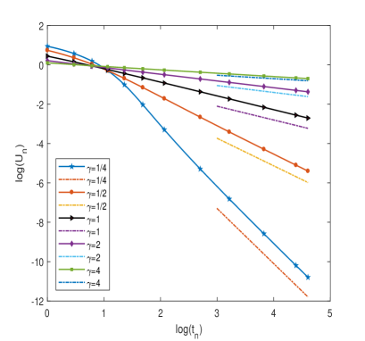
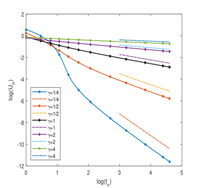
In this test, consider the scalar model (4): Dtαy(t)+νtβy(t)γ=0D_{t}^{\alpha}y(t)+\nu t^{\beta}y(t)^{\gamma}=0 with initial value y(0)=y0>0y(0)=y_{0}>0 and β>α\beta>-\alpha, which has an optimal numerical decay rates O(tn(α+β)/γ)O\left(t_{n}^{(\alpha+\beta)/\gamma}\right) predicted by Theorem 4.1.

Here we take m=5m=5, u0=5u_{0}=5 and the parameter γ={1/4,1/2,1,2,4}\gamma=\{1/4,1/2,1,2,4\}. Table 1 and Table 2 respectively show the polynomial decay rate of the numerical solution computed by Grünwald-Letnikov scheme for various parameters of α\alpha and β\beta. We also plot the log-log relation of the numerical solution UnU_{n} and tnt_{n} in Figure 1 with various parameters. It can be seen from those data and Figure that the numerical solutions are monotone and positive and are completely consistent with our theoretical prediction, i.e. rα(tn)α+βγr_{\alpha}^{*}(t_{n})\sim\frac{\alpha+\beta}{\gamma}.

Table 1: Observed rα(tn)r^{*}_{\alpha}(t_{n}) for tn=2000,4000,6000,8000,10000t_{n}=2000,4000,6000,8000,10000 with β=0.3\beta=0.3, α=0.4\alpha=0.4
tnt_{n} γ=1/4\gamma=1/4 γ=1/2\gamma=1/2 γ=1\gamma=1 γ=2\gamma=2 γ=4\gamma=4
20002000 2.801315 1.400861 0.700384 0.348185 0.172802
40004000 2.800657 1.400434 0.700247 0.348575 0.173056
60006000 2.800438 1.400291 0.700191 0.348764 0.173191
80008000 2.800328 1.400219 0.700158 0.348883 0.173282
1000010000 2.800263 1.400176 0.700137 0.348967 0.173348
rαr_{\alpha}^{*} 2.8 1.4 0.7 0.35 0.175
Table 2: Observed rα(tn)r^{*}_{\alpha}(t_{n}) for tn=2000,4000,6000,8000,10000t_{n}=2000,4000,6000,8000,10000 with β=0.3\beta=-0.3, α=0.8\alpha=0.8
tnt_{n} γ=1/4\gamma=1/4 γ=1/2\gamma=1/2 γ=1\gamma=1 γ=2\gamma=2 γ=4\gamma=4
20002000 2.001509 1.001087 0.502494 0.250823 0.124179
40004000 2.000754 1.000559 0.501724 0.250673 0.124242
60006000 2.000503 1.000379 0.501393 0.250602 0.124278
80008000 2.000378 1.000288 0.501199 0.250556 0.124303
1000010000 2.000302 1.000232 0.501067 0.250524 0.124322
rαr_{\alpha}^{*} 2 1 0.5 0.25 0.125
Refer to caption
Refer to caption
Figure 1: Logarithm of numerical solutions log(Un)\log(U_{n}) for γ=1/4,1/2,1,2,4\gamma=1/4,1/2,1,2,4 with β=0.3\beta=0.3, α=0.4\alpha=0.4 (left) and β=0.3\beta=-0.3, α=0.8\alpha=0.8 (right).

5.2 Time fractional PDEs with time-dependent coefficients

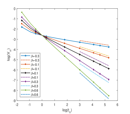
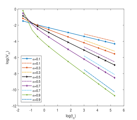
Consider the time fractional partial differential equation:

{Dtαu(t,x)tβΔu(t,x)=tβ(1+t)α+βfort>0andxΩ,u(t,x)=0fort>0andxΩ,u(0,x)=u0(x)forxΩ,\left\{\begin{aligned} &D_{t}^{\alpha}u(t,x)-t^{\beta}\Delta u(t,x)=\frac{t^{\beta}}{(1+t)^{\alpha+\beta}}~{}~{}for~{}t>0~{}and~{}x\in\Omega,\\ &u(t,x)=0~{}~{}for~{}t>0~{}and~{}x\in\partial\Omega,\\ &u(0,x)=u_{0}(x)~{}~{}for~{}x\in\Omega,\end{aligned}\right. (52)

where 𝒩(u)=Δu\mathcal{N}(u)=\Delta u is Laplace operator. One has the Poincaré inequality u(t,)L2(Ω)κ(Ω|u(t,)|2𝑑x)1/2\|u(t,\cdot)\|_{L^{2}(\Omega)}\leq\kappa(\int_{\Omega}|\bigtriangledown u(t,\cdot)|^{2}dx)^{1/2} for some positive constant κ>0\kappa>0, i.e., the structural assumption (2) holds true for s=2,γ=1s=2,~{}\gamma=1. Therefore, we can obtain that the decay rate of the true solution is O(t(α+β))O(t^{-(\alpha+\beta)}).

In this example, we take Ω=[0,1]2\Omega=[0,1]^{2} and the initial value u0(x1,x2)=10sin(πx1)sin(πx2)u_{0}(x_{1},x_{2})=10\sin(\pi x_{1})\sin(\pi x_{2}). The linear finite element in space and Grünwald-Letnikov scheme in time are employed to solve the problem (52) with time step size τ=0.1\tau=0.1. Table 3 and Table 4 presents the results of the decay rate for numerical solutions with β=0.3,0.1,0.1,0.3,0.6\beta=-0.3,~{}-0.1,~{}0.1,~{}0.3,~{}0.6, α=0.5\alpha=0.5 and β=0.3\beta=0.3, α=0.1,0.3,0.5,0.7,0.9\alpha=0.1,~{}0.3,~{}0.5,~{}0.7,~{}0.9 to problem (52). Both log-log picture presented in Figure 2 show the evolution of Vn:=UnL2(Ω)V_{n}:=\|U_{n}\|_{L^{2}(\Omega)} has decay rate tn(α+β)t_{n}^{-(\alpha+\beta)}, which are also completely consistent with our theoretical prediction

Table 3: Observed rα(tn)r^{*}_{\alpha}(t_{n}) for tn=20,60,100,140,180t_{n}=20,60,100,140,180 with β=0.3,0.1,0.1,0.3,0.6\beta=-0.3,~{}-0.1,~{}0.1,~{}0.3,~{}0.6, and α=0.5\alpha=0.5
tnt_{n} β=0.3\beta=-0.3 β=0.1\beta=-0.1 β=0.1\beta=0.1 β=0.3\beta=0.3 β=0.6\beta=0.6
2020 0.203591 0.403624 0.603672 0.803713 1.103757
6060 0.201189 0.401221 0.601252 0.801270 1.101281
100100 0.200701 0.400732 0.600756 0.800768 1.100773
140140 0.200491 0.400521 0.600542 0.800551 1.100554
180180 0.200375 0.400404 0.600423 0.800430 1.100432
rαr_{\alpha}^{*} 0.2 0.4 0.6 0.8 1.1
Table 4: Observed rα(tn)r^{*}_{\alpha}(t_{n}) for tn=20,60,100,140,180t_{n}=20,60,100,140,180 with β=0.3\beta=0.3, and α=0.1,0.3,0.5,0.7,0.9\alpha=0.1,~{}0.3,~{}0.5,~{}0.7,~{}0.9
tnt_{n} α=0.1\alpha=0.1 α=0.3\alpha=0.3 α=0.5\alpha=0.5 α=0.7\alpha=0.7 α=0.9\alpha=0.9
2020 0.400381 0.601848 0.803713 1.005938 1.208512
6060 0.400083 0.600622 0.801270 1.002020 1.202882
100100 0.400029 0.600372 0.800768 1.001218 1.201734
140140 0.400008 0.600265 0.800551 1.000872 1.201240
180180 0.400000 0.600205 0.800430 1.000679 1.200965
rαr_{\alpha}^{*} 0.4 0.6 0.8 1 1.2
Refer to caption
Refer to caption
Figure 2: Logarithm of numerical solutions log(Vn)\log(V_{n}) for β=0.3,0.1,0.1,0.3,0.6\beta=-0.3,-0.1,~{}0.1,~{}0.3,~{}0.6, α=0.5\alpha=0.5 (left) and β=0.3\beta=0.3, α=0.1,0.3,0.5,0.7,0.9\alpha=0.1,~{}0.3,~{}0.5,~{}0.7,~{}0.9 (right).

References

  • [1] M. Bologna, A. Svenkeson, B. J. West, and P. Grigolini. Diffusion in heterogeneous media: An iterative scheme for finding approximate solutions to fractional differential equations with time-dependent coefficients. J. Comput. Phys., 293:297–311, 2015.
  • [2] T. Boudjeriou. Decay estimates and extinction properties for some parabolic equations with fractional time derivatives. Fract. Calc. Appl. Anal., 27:393–432, 2024.
  • [3] F. S. Costa, E. C. Oliveira, and A. R. G. Plata. Fractional diffusion with time-dependent diffusion coefficient. Rep. Math. Phys., 87:59–79, 2021.
  • [4] S. Dipierro, E. Valdinoci, and V. Vespri. Decay estimates for evolutionary equations with fractional time-diffusion. J. Evol. Equ., 19:435–462, 2019.
  • [5] K. S. Fa and E. K. Lenzi. Time-fractional diffusion equation with time dependent difussion coefficient. Phys. Rev. E (3), 72:011107, 2005.
  • [6] D. Hernández and E. C. Herrera-Hernández. Non-local diffusion models for fractured porous media with pressure tests applications. Adv. Water Resour., 149:103854, 2021.
  • [7] J. Hristov. Subdiffusion model with time-dependent diffusion coefficient: Integral-balance solution and analysis. Therm. Sci., 21:69–80, 2017.
  • [8] B. Jin. Fractional differential equations: An approach via fractional derivatives. Springer, Cham, 2021.
  • [9] Bangti Jin and Zhi Zhou. Numerical treatment and analysis of time-fractional evolution equations, volume 214. Springer Nature, 2023.
  • [10] J. Kemppainen and R. Zacher. Long-time behavior of non-local in time Fokker-Planck equations via the entropy method. Math. Models Methods Appl. Sci., 29:209–235, 2019.
  • [11] Natalia Kopteva. Error analysis of the L1 method on graded and uniform meshes for a fractional-derivative problem in two and three dimensions. Math. Comp., 88(319):2135–2155, 2019.
  • [12] L. Li and D. L. Wang. Complete monotonicity-preserving numerical methods for time fractional odes. Commun. Math. Sci., 19:1301–1336, 2021.
  • [13] H. L. Liao, W. McLean, and J. W. Zhang. A discrete gronwall inequality with applications to numerical schemes for subdiffusion problems. SIAM J. Numer. Anal., 57(1):218–237, 2019.
  • [14] A. G. Smadiyeva and B. T. Torebek. Decay estimates for the time-fractional evolution equations with time-dependent coefficients. Proc. R. Soc. A, 479:381–397, 2023.
  • [15] Martin Stynes. A survey of the L1 scheme in the discretisation of time-fractional problems. Numer. Math. Theor. Meth. Appl., 15:1173–1192, 2022.
  • [16] V. Vergara and R. Zacher. Optimal decay estimates for time-fractional and other nonlocal subdiffusion equations via energy methods. SIAM J. Math. Anal., 47:210–239, 2015.
  • [17] D. L. Wang and M. Stynes. Optimal long-time decay rate of numerical solutions for nonlinear time-fractional evolutionary equations. SIAM J. Numer. Anal., 61:2011–2034, 2023.
  • [18] D. L. Wang and J. Zou. Mittag-Leffler stability of numerical solutions to time fractional odes. Numer. Algorithms, 92:2125–2159, 2023.
  • [19] R. Zacher. Boundedness of weak solutions to evolutionary partial integro-differential equations with discontinuous coefficients. J. Math. Anal. Appl., 348:137–149, 2008.