Mitigating Domain Mismatch in Face Recognition Using Style Matching
Abstract
Despite outstanding performance on public benchmarks, face recognition still suffers due to domain mismatch between training (source) and testing (target) data. Furthermore, these domains are not shared classes, which complicates domain adaptation. Since this is also a fine-grained classification problem which does not strictly follow the low-density separation principle, conventional domain adaptation approaches do not resolve these problems. In this paper, we formulate domain mismatch in face recognition as a style mismatch problem for which we propose two methods. First, we design a domain discriminator with human-level judgment to mine target-like images in the training data to mitigate the domain gap. Second, we extract style representations in low-level feature maps of the backbone model, and match the style distributions of the two domains to find a common style representation. Evaluations on verification and open-set and closed-set identification protocols show that both methods yield good improvements, and that performance is more robust if they are combined. Our approach is competitive with related work, and its effectiveness is verified in a practical application.
keywords:
face recognition , domain adaptation , style transfer , Sinkhorn algorithm , optimal transport1 Introduction
Face recognition is an efficient tool for identity authentication. When implemented using deep learning, its performance is nearly perfect on public benchmarks, and it can be used in applications as varied as social media, surveillance, police, and military. However, as shown persuasively in Phillips [1], in real-world deployments, powerful face recognition models usually exhibit poor performance, regardless of the amount of training data. This is primarily due to domain mismatch, that is, the mismatch between the training data (the source domain) and testing data (target domain) distributions. Such mismatch can be caused by differences in illumination, race, gender, or age. One solution is to fine-tune the model on the target domain with supervised training, but labeling is expensive, and it is impossible to collect labeled data that covers all possible scenarios. The problem is thus how best to adapt the model by leveraging unlabeled data in the target domain.
Although many studies have been conducted on this problem, most assume that the domains are shared classes. The premise of face recognition, however, is the opposite. In general, identities in a scenario do not constitute a training dataset, which leads to an unique problem in face recognition. Therefore, of the few studies on domain mismatch for face recognition [2, 3, 4, 5, 6, 7, 8], most adopt domain adaptation approaches. According to Yosinski et al. [9], for convolutional neural networks (CNNs), as lower layers are more transferable, the main idea for classical domain adaptation is to fine-tune parameters by aligning the feature distributions of the two domains in higher layers. They achieve modest improvements under the low-density separation assumption. In contrast to objects, the contour variation among human faces is low, which means that face recognition is a kind of fine-grained classification problem. Since feature distributions of unseen identities do not necessarily satisfy the low-density separation assumption, domain mismatch in face recognition should be accounted for at the texture level.
One technique for domain adaptation is to adapt source images to appear as if drawn from the target domain [10, 11, 12] and to fine-tune the model with the transferred images to reduce the domain gap. With the advance of generative adversarial networks (GAN) [13], it is possible to synthesize precise facial images [14, 15, 16]. Thus it would seem that GANs could be used to reduce face recognition domain mismatch, but using GANs to transfer source images could lead to two problems. First, if non-face images are generated, learning would be harmed. Second, the styles in both domains should be diverse, but as style is not easily defined, it is difficult to determine which target style a source image should be transferred to. Transferring each source image to the styles of all target images would incur a complexity of . The GAN must be large enough to generate high-quality images, and there must be a sufficient number of identities and images in the training data. This would however preclude the transfer of all the source images in a reasonable amount of time.
In this paper, we propose a feasible method for style-based (or, equivalently, texture-level) model adaptation. We follow Zhang et al. [17] in adopting a domain discriminator with human-level judgment to evaluate the similarity of a source image to the target domain. Also, per Chu et al. [18], Wu et al. [19], and Liu et al. [20], we utilize evaluations to up-weight source images that are visually similar to target images. This adaptation mechanism is called perceptual scoring (PS). The style of an image can be represented by feature map statistics from lower to higher CNN layers [21, 22, 23, 15]. We adopt Sinkhorn divergence [24, 25, 26, 27, 28, 29, 30] to align the style distributions of the source and target domains as if the convolutional layers are learned to produce a common style space in which source and target images are visually similar. This results in shallow-layer feature maps which are domain-invariant. We term this approach style matching (SM).
To evaluate the performance of the proposed approaches, we conduct evaluations on IJB-A/B/C [31, 32, 33] since they provide comprehensive face verification, closed-set identification, and open-set identification protocols, facilitating evaluations under various scenarios. The effectiveness of our approach is competitive with that of related work on domain adaptation for face recognition. Moreover, to understand whether the proposed approaches are capable of solving real world problems, we apply them to a surveillance application in the library of National Chiao Tung University (NCTU). The testing results show that the proposed approaches can improves a baseline model by a large margin.
The contributions in this research can be summarized as follows:
-
1.
We conduct a comprehensive study of domain adaptation for face recognition, showing that most domain adaptation techniques do not apply to face recognition. If adaptation algorithms for face recognition are designed at the texture level, domain mismatch can be formulated as a style mismatch problem.
-
2.
We propose perceptual scoring with human-level judgment to enhance the learning of visually target-like source images. Style matching adapts the model by learning a common style space in which the style distributions of both domains are confused.
-
3.
We conduct comprehensive testing protocols to cover all possible applications of face recognition to evaluate models objectively. Experiment results demonstrate the competitiveness of the proposed approaches.
-
4.
We apply the proposed approaches to a real scenario, and show the significant improvements compared with the baseline.
The rest of this paper is structured as follows: In Section 2, we briefly review related work on face recognition and domain adaptation. Then, in Section 3, we describe in detail the proposed approaches, and in Section 4 we explain the evaluation protocols for different scenarios. In Section 5, we explain the experimental settings, analyze the testing results, and compare these with prior work. We conclude in Section 6.
2 Related Work
2.1 Face Recognition
After deep CNN-based face recognition [34] successfully surpassed conventional methods by a large margin on a famous benchmark [35], this became the major backbone of face recognition [36]. DeepID [37, 38, 39] improves classification loss with contrastive loss [40] to learn a discriminative embedding space. Triplet loss [41] separates positive pairs from negative samples via a distance measure, and is free from classification loss. Learning embeddings without a classifier is known as metric learning [42]. Such a learning strategy relies heavily on good data mining methods. Schroff et al. [41] adopt hard sample mining to learn informative triplets. Center loss [43] reduces intra-class variation by regressing features to their cluster centers. To further separate inter-class samples, many margin penalty losses have been proposed, including SphereFace [44], CosFace [45], and ArcFace [46]. As presented in Deng et al. [46], classification loss with a suitable margin penalty significantly improves performance. Thus determining a good margin is an active research focus. Liu et al. [47] learn margins by maximizing them in total loss. Fair loss [48] involves using a policy network trained by reinforcement learning to control margins according to the samples in the current batch. Huang et al. [49] change the loss adaptively by evaluating the relation between intra- and inter-class similarities.
Despite the nearly perfect accuracy achieved by these methods, their performance depends on huge labeled datasets to achieve better generalization, and thus methods in this line of research cannot be used to account for domain mismatch.
2.2 Domain Adaptation
The aim of domain adaptation is to leverage unlabeled data to fine-tune a trained model for the target domain; source data labels are assumed to be available [50]. The main challenge with domain adaptation is domain mismatch, that is, dissimilar distributions for the two domains, which degrades model performance in the target domain. To eliminate this domain gap, some focus on modifying the classifier’s decision boundary [18], while others focus on learning an embedding space in which the distributions of the two domains are aligned [51, 52, 53, 19, 54, 55, 56]. Target-domain performance can be refined by observing the low-density separation principle. Since aligning distributions does not fully satisfy the assumption that domains are shared classes, studies have been conducted on developing better distribution matching methods. Maximum mean discrepancy (MMD) has been widely adopted for domain adaptation [51, 53]. By mapping features to a reproducing kernel Hilbert space (RKHS), we can estimate the domain discrepancy through the squared distance between kernel mean embeddings. In Long et al. [51, 53], MMD is used to match feature distributions on deeper CNN layers. Yan et al. [57] weight MMD by class information to better match the feature distributions. Although MMD is simple and effective, it tends to focus on matching high-density regions [27]. The success of GANs [13] has revealed adversarial learning as another option [54, 55, 56]: a domain discriminator is created to judge the domain of each sample. For training, this results in learning an embedding space to fool the domain discriminator, which results in the distributions being confused. Although adversarial learning based approaches achieve improved performance, they still involve the training of extra parameters (for the discriminator). Also, in many approaches, the two models are trained interactively, which complicates the setting of proper hyperparameters for training.
2.3 Domain Adaptation for Face Recognition
Face recognition is a fine-grained classification problem for which the classes (identities) in the source and target domains are not the same. Hence, conventional domain adaptation methods cannot be used for face recognition. There is a paucity of research on domain adaptation for face recognition.
2.3.1 Distribution Matching
2.3.2 Clustering
To make up for the shortcomings of distribution matching, clustering is used to assign pseudo labels in the target domain. In Wang and Deng [3], a target-domain classifier is trained using pseudo labels. Following the low-density separation principle, Wang et al. [4] use mutual information loss to categorize target-domain embeddings. Leveraging frame consistency in video face recognition, Arachchilage and Izquierdo [5] better estimate positive and negative pairs of target images. After clustering and mining, the model is fine-tuned using a modified version of triplet loss. Similar work is described in Arachchilage and Izquierdo [8]. As clustering-based methods rely on the target domain priors, hyperparameters must be determined before clustering, which is difficult in practice.
2.3.3 Instance Normalization
In work on style transfer [21, 22, 23, 15], instance normalization is used for style normalization. This could also be a way to learn a domain-invariant model. Li et al. [58] remove bias by taking the mean and standard deviation from the target domain as batch normalization parameters. Qing et al. [59] combine instance and batch normalization (IBN) to improve cross-domain recognition. Nam et al. [60] propose batch-instance normalization (BIN), summing instance and batch normalization with an optimal ratio; they thus yield superior results by learning the ratio between two operators. In Qian et al. [61], the IBN layer is adopted as the domain adaptation layer, and the ratio between batch and instance normalization is determined by the domain statistics. Drawing from these studies, Jin et al. [62] propose style normalization and restitution (SNR), extracting domain-invariant features and preserving task-relevant information to further improve performance. However, these approaches necessitate changes to the network architecture that incur a far greater computational complexity.
3 Proposed Approach

With domain adaptation, the training dataset is taken as the source domain, denoted by , and the testing dataset is taken as the target domain, denoted by . There are images in the source domain, and images in the target domain. The source and target images are and respectively. Each has a label which uses one-hot encoding. The target image labels are unknown, reflecting the need for domain adaptation. To simplify the notation, , , and stand for an arbitrary image, a source image, and a target image respectively.
In general face recognition, the source and target domain are not shared classes, and the task is fine-grained categorization. In this case, short feature distances between two images do not imply that they are visually similar. We account for this by treating domain mismatch as style mismatch. We propose two approaches under different perspectives: perceptual scoring (PS) and style matching (SM). We outline the proposed approach in Fig. 1. For PS we draw from Zhang et al. [17] in the use of a domain discriminator, which judges the domain discrepancy of an image through a perceptual metric, to facilitate the learning of source images which are visually similar to the target images. In SM, given a baseline face recognition model , we extract style features from convolutional feature maps, and align the distributions of style features from the two domains. Thus the face recognition model generates convolutional features with homogeneous styles and focuses on learning target-like source images to improve testing performance.
The rest of this section is structured as follows. In the next subsection, we describe the primary classification loss with which we train the model by source images with the supervision of labels. In the second and third subsections, we describe the PS and SM methods respectively, after which we summarize the two style-based domain adaptation methods.
3.1 Classification Loss
For visual recognition, the goal of an embedding function is to encode images to an embedding space in which similar images are close together and dissimilar images are far apart so that we can judge how similar two given images are, or which category an image belongs to. The easiest way to train an embedding function is to use an additional classifier. The embedding function is modeled by a convolutional neural network, , and the classifier is a single-layer perceptron (a matrix) followed by softmax, . Since the output of the classifier is a probability distribution, we train the cascaded model, , by minimizing cross entropy. The training loss is expressed as
| (1) |
which is termed classification loss. We use this to train a baseline model from scratch and preserve inter-class distances when adapting the model.
3.2 Perceptual Scoring
Assuming that domain information is shared between two domains, we draw from Chu et al. [18], Wu et al. [19], and Liu et al. [20] by mining informative images in the training dataset to mitigate domain shift.
3.2.1 Domain Discriminator
The architecture from Zhang et al. [17] is modified as the domain discriminator, as shown in Fig. 2. This discriminator approximates human-level judgments to calculate a score that represents how similar an image is to the target domain. For image , a feature stack is extracted from layers of a backbone network and unit-normalized in the channel dimension, denoted by for layer . Each is scaled by vector and summed channel-wise. We average spatially to yield a scalar representation on each layer:
| (2) |
where is a convolution operator. We then concatenate the representations to produce a perceptual feature , which we pass through a single-layer perceptron (vector ) followed by a sigmoid activation to judge the input image. The domain discriminator is expressed as
| (3) |
Note that since we use SqueezeNet [63] as the backbone network, in our case .

3.2.2 Training and Adaptation
We sample images from the source and target domains equally and use the following loss function (domain discrepancy loss) to train the domain discriminator:
| (4) |
in which we expect the discriminator to produce a low score (tending to 0) for a source image but a high score (tending to 1) for a target image. This score is used in the classification loss in Equation 1 to up-weight the loss caused by target-like images. The classification loss is modified as
| (5) |
where is the loss for adapting the model based on PS.
3.3 Style Matching
Although PS indirectly reduces domain shift, its premise limits performance due to a lack of target-like images in the training dataset. To compensate for this weakness, with SM we seek a common space in which the style distributions of two domains are aligned.
3.3.1 Style Measures
According to studies on style transfer [21, 22, 23, 15], the stacks of mean and standard deviation on the feature maps describe the style of an image. For layer in the face recognition model, the style representation is designated as . The measures of styles from the two domains are defined as
| (6) |
| (7) |
where and are measures of , and and are measures of . We seek to minimize a certain distribution matching loss between , and .
3.3.2 Matching Distribution
In the literature on domain adaptation, MMD and adversarial learning are the main ways to match distributions. Although MMD is simple and necessitates no extra training parameters, it focuses on matching the region of high density [27], which may incur greater bias. Adversarial learning approaches, however, approximate relative entropy or the Wasserstein distance (optimal transport) by training the embedding function and the discriminator interactively. Although adversarial learning yields a better estimation of domain discrepancy, it requires extra parametric subnetworks, which complicates training. We strike a balance between the two methods by calculating the distribution matching loss using Sinkhorn divergence [24, 25, 26, 27, 28, 29, 30], which interpolates optimal transport and MMD, and has been successfully applied to generative models in Genevay et al. [64].
3.3.3 Sinkhorn Divergence
Similar to Genevay et al. [64], we align the style distributions of the source and target domains by minimizing
| (8) |
where . Here, and are samples from distributions and respectively. Where is some exponent, is a cost equipped with a distance function . We define as Euclidean distance, and set . The entropy-regularized optimal transport, that is, Wasserstein distance, is , in which factor regularizes entropy. Thus can be treated as a mass-moving plan between and . As expressed in Cuturi [24], Cuturi and Doucet [25], and Genevay et al. [64], regularized optimal transport is equivalent to restricting the search space by using the scaling form of :
| (9) |
where ; the role of here mirrors that of bandwidth in MMD. The optimization problem of Equation 8 turns into finding and that meet certain requirements. Based on the Sinkhorn algorithm [24, 25], and can be found by
| (10) |
where the fraction here is element-wise division. Starting with , we obtain feasible and after iterations. The budget is set to according to Genevay et al. [64]. Hence, Equation 8 can be modified as
| (11) |
where is an element-wise multiplication operator. Since can be large, to prevent numerical explosions during training, we divide by to normalize the total cost. However, such a discrepancy approximation tends to overfit. To account for this, we add intra-measure Wasserstein distance to penalize the inter-measure Wasserstein distance:
| (12) |
where is called Sinkhorn loss in Genevary et al. [64].
3.3.4 Style Matching Loss
We adopt Sinkhorn loss in Equation 12 to match the style distributions of the source and target domains, so the style matching loss can be expressed as
| (13) |
where is the number of adaptation layers in .
3.4 Style-based Adaptation
Since style matching loss in Equation 13 requires the supervision of classification loss to learn categorization, adaptation loss with style matching is defined as
| (14) |
where is a Lagrange multiplier. In the experiments, to prevent from dominating the total loss, we set to make the product of less than . The complete loss proposed in this paper consists of both PS and SM:
| (15) |
By minimizing , we adapt a model from the source domain to the target domain from a style perspective.
4 Evaluations
The two major applications of face recognition are face verification and identification, of which face identification further divides into closed-set and open-set identification. The performance of a model across different scenarios must be evaluated under different protocols.
4.1 Verification
The task of verification is to judge whether the given two facial images are the same identity. The two major evaluation protocols are described below.
4.1.1 K-fold Cross Validation
In this protocol, to avoid bias, the numbers of positive and negative pairs are usually the same, such as in the Labeled Faces in the Wild (LFW) [35, 65] and YouTube Faces (YTF) [66] datasets. The dataset is divided into partitions. We evaluate the model on each partition by using the optimal threshold found by testing all the other partitions, and average the accuracies.
4.1.2 True Positive Rate under False Positive Rate
We determine the threshold for rejecting negative pairs that corresponds to the desired false positive rate (FPR) or false alarm rate (FAR), which yields a true positive rate (TPR) that represents the accuracy on positive pairs. In general, there are far more negative pairs than positive pairs to test the robustness of a model.
4.2 Closed-set Identification
Given a facial image, usually called the probe, the goal of face identification is to determine its identity by finding the most similar facial images in a gallery. In the case of closed-set identification, the identities of the probes must be a subset of the identities in the gallery. Therefore, rank-K (or top-K) accuracy is employed to evaluate the performance under this scenario. For each probe, we compute the similarities of all images in the gallery with respect to the probe, and sort these similarities from high to low. If the similarity between the probe and images of the same identity is ranked in the top-K, this identity is taken to be the correct prediction. After testing all the probes, rank-K accuracy is obtained as the ratio of correct predictions.
4.3 Open-set Identification
In open-set identification, the identities of probes may not be found in the gallery, in which case the task is not only to determine the identity of a given probe but also to report failure if the identity of the probe is not enrolled in the gallery. To evaluate the performance of open-set identification, we first set a threshold by which to reject probes with unknown identities under an acceptable FAR; in this case, this is the false positive identification rate (FPIR). Based on the set threshold, our metric is rank-1 accuracy, that is, the true positive identification rate (TPIR).
5 Experiments
5.1 Datasets
The datasets utilized here are listed in Table 1. Created for different purposes, they can be divided into three types:
5.1.1 Training
VGGFace2 [67] and CASIA-WebFace [68] are our training datasets; all facial images in both datasets were captured in the wild. Due to the large number of images for each identity in VGGFace2, it ensures better learning than CASIA-WebFace, even though it contains fewer identities. As in most of the relevant literature [6, 2, 3, 4], CASIA-WebFace is a primary source dataset in this paper. Following Wang et al. [3] and Arachchilage and Izquierdo [8], we initialize the backbone model on VGGFace2 after which we fine-tune the parameters on CASIA-WebFace.
5.1.2 Validation
We use LFW [35], CFP-FP [69], and AgeDB-30 [70] as the validation datasets; for each we use a 10-fold cross validation protocol. Their small size facilitates efficient model evaluations. When training a baseline model, we test it on these datasets after every epoch. After training, we pick the model whose average accuracy is the highest of all the generations as the baseline model.
5.1.3 Testing
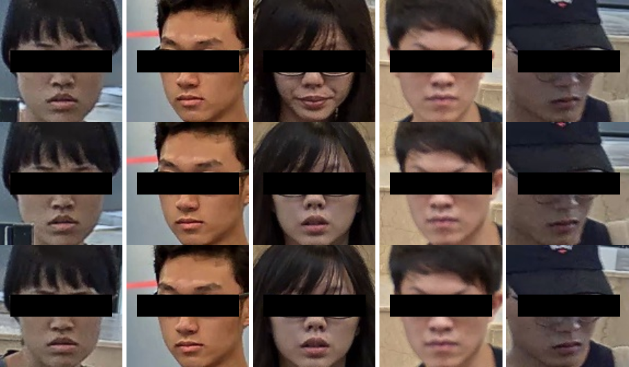
IJB-A [31] is a joint face detection and recognition dataset that contains a mixture of still images and videos under challenging conditions, including blur as well as large pose and illumination variation. It provides 10-split evaluation protocols containing both verification and identification. We take the average of the 10-split evaluations as the final results. IJB-A was extended as IJB-B [32], which was further extended as IJB-C [33]. The evaluation methods in IJB-B and IJB-C are the same. In terms of verification, only one protocol is provided, but the positive-versus-negative pairs in IJB-B and IJB-C are about 10K/8M and 19.6K/15.6M respectively, which is more challenging than that of IJB-A (1.8K/10K), as listed in Table 2. For identification, both provide one probe set and two gallery sets for evaluation. We successively test each gallery set using the probe set and use their average as the final result. YTF [66] contains 3,425 videos from 1,595 identities, for a total of 621.2K frames. As with the validation datasets, its protocol follows 10-fold cross validation, in which each fold is composed of 250 positive and negative pairs. Furthermore, we cooperate with the library of National Chiao Tung University (NCTU) for surveillance application. A system was built to collect the data automatically. When a subject entered the library, the system recorded and labeled the video by the student or staff identity card. Due to personal information protection, the labels are anonymous. To eliminate the interference of head pose variation, we adopted the head pose estimation model in Hsu et al. [71] to filter out the frames with large head pose (pitch, roll, or yaw ). This dataset is called NCTU-Lib, and its samples are shown in Fig. 3. The domain discrepancy between the training dataset and NCTU-Lib is large since almost all subjects in NCTU-Lib are Asian, which makes it more difficult to adapt the model.
Ver=verification, ID=identification.
Dataset Protocol Identities Images Images/identity Ver ID VGGFace2 [67] 9,131 3.31M 362.6 CASIA-WebFace [68] 10,575 494.4K 46.8 LFW [35] ✓ 5,749 13,233 2.3 CFP-FP [69] ✓ 500 7,000 14 AgeDB-30 [70] ✓ 568 16,488 29 IJB-A [31] ✓ ✓ 500 25.8K 51.6 IJB-B [32] ✓ ✓ 1,845 76.8K 41.6 IJB-C [33] ✓ ✓ 3,531 148.8K 42.1 YTF [66] ✓ 1,595 621.2K 389.5 NCTU-Lib ✓ ✓ 6,187 105.1K 17.0
Dataset Verification Identification Positive Pairs Negative Pairs Subjects (Gallery) Samples/Subjects (Probe) Known Unknown YTF [66] 250 250 - - IJB-A [31] 1.8K 10K 112 1.2K/112 0.6K/55 IJB-B [32] 10K 8M 922 5.1K/922 5.1K/922 IJB-C [33] 19.6K 15.6M 1.77K 9.8K/1.77K 9.8K/1.8K NCTU-Lib 4.4K 3.2M 3.16K 6.0K/3.16K 3.0K/3.0K
5.2 Implementation Details
Here, we describe the image preprocessing, feature processing, baseline model training, source and target dataset definitions, and training using the proposed domain adaptation methods.
5.2.1 Processing of Images and Features
If the multitask convolutional neural network (MTCNN) [72] detects a face in an image, we align the face to the fixed reference points using the eyes, mouth corners, and nose center. If it fails, we decide what to do based on the dataset. We ignore the training datasets and YTF since there is plenty of data for training and testing. For IJB-A/B/C, if three landmarks (eyes and nose center) are provided, we align these to the same reference points of the same landmarks, or we apply a square box whose side is half of the maximal side of the image to crop on the center. All processed images are resized to and cropped to for testing. When training, we augment the images by mirroring them with probability, and resize them to and randomly crop them to . In evaluations, we follow Whitelam et al. [32] when fusing the features. That is, in a template, the frames of each type of media (still images or video frames) are averaged before all medias are averaged.
5.2.2 Baseline Model and Source Dataset
We used MobileFaceNet [73] as our backbone model. Equation 1 is the primary classification loss in this paper. As mentioned above, the model was first trained on VGGFace2 dataset [67]. We used stochastic gradient descent (SGD) with momentum to train all models. The training epochs, batch size, learning rate, and momentum were set to 50, 128, 0.1, and 0.9 respectively, and the learning rate was divided by 10 every 12 epochs. After that, when transferring to CASIA-WebFace dataset [68], the learning rate was set to 0.01 to warm up the classifier by one epoch before fine-tuning all parameters. We then set the learning rate to 0.0001 to fine-tune the parameters, and again divided by 10 every 12 epochs. The other settings remained unchanged. The backbone model fine-tuned on CASIA-WebFace was then used as the baseline model denoted by softmax.
5.2.3 Target Dataset
We assumed that the IJB-A/B/C datasets [31, 32, 33] are shared domain information. Only IJB-A was used as the target dataset when testing on these datasets. We used all images and frames in IJB-A to adapt the model. Similarly, when testing on the YTF dataset [66], we used all the frames of each video in YTF. During adaptation, the learning rate was also set to 0.0001 to fine-tune the baseline model; other settings remained unchanged.
5.2.4 Regularizing Entropy for Style Matching
Since the role of is similar to bandwidth in MMD, we followed related studies [74, 2, 3] to set its value. Luo et al. [2] and Wang et al. [3] suggest setting the bandwidth to the median pairwise distance on source dataset. However, such an exhaustive search is not practical since training datasets are usually large. This can instead be estimated by a Monte Carlo method, but we propose a more efficient way to determine the value. Similar to the learning process in batch normalization, we estimated by the mean pairwise distance between source and target samples in a mini-batch, and updated it every iteration by
| (16) |
where is the current estimation. Momentum was set to . In the following experiments, we compare the dynamic (the proposed method) and the fixed .
5.2.5 Definition of Adaptation Layers
MobileFaceNet [73] is described in Table 3. For the following experiments, we mainly used four adaptation layers in shallow networks for SM. From shallow to deep, the dimensions of the feature maps were (), (), (), and () respectively.
Operator Input Output Convolution - Depth-wise convolution 1 Bottleneck 2 Bottleneck 3 Bottleneck 4 Bottleneck 5 Bottleneck 6 Bottleneck 7 Convolution 8 Linear depth-wise convolution 9 Linear convolution 10
5.3 Ablation Study
The values in boldface are the best in the row, and underlined values in boldface are the best in the column.
Method IJB-A TPR (%) IJB-B TPR (%) IJB-C TPR (%) FPR=0.0001 FPR=0.001 FPR=0.01 FPR=0.1 FPR=0.0001 FPR=0.001 FPR=0.01 FPR=0.1 FPR=0.0001 FPR=0.001 FPR=0.01 FPR=0.1 Baseline softmax 52.23 75.63 90.54 96.88 68.91 83.61 93.43 98.22 74.04 86.44 94.59 98.54 Perceptual scoring softmax FF PS 54.60 77.67 91.02 96.88 70.29 84.15 93.74 98.32 75.02 87.00 94.92 98.61 softmax PS 55.00 78.43 91.17 96.92 71.16 84.58 93.75 98.27 75.82 87.21 94.90 98.58 Style matching softmax SM , fixed 65.64 82.72 92.46 96.96 74.65 86.69 95.02 98.42 78.68 89.17 95.90 98.75 softmax SM 64.83 82.28 92.23 96.96 75.09 86.86 94.99 98.45 78.98 89.30 95.86 98.72 softmax SM 65.81 83.67 92.48 96.92 74.83 86.97 95.08 98.49 79.15 89.50 95.94 98.76 softmax SM 66.33 82.49 92.06 96.91 75.58 87.08 94.89 98.38 79.46 89.51 95.80 98.71 softmax SM 67.64 83.28 92.23 96.89 74.95 87.22 94.93 98.43 79.81 89.58 95.83 98.75 Combination softmax SM + PS 66.88 83.53 92.48 97.05 75.24 87.06 95.15 98.47 79.76 89.56 96.07 98.78 softmax SM + PS 67.78 84.31 92.65 97.03 75.96 87.55 95.08 98.50 80.19 89.85 95.99 98.79 softmax SM + PS 68.70 83.52 92.30 96.82 75.51 87.32 95.00 98.48 79.83 89.83 95.92 98.78 softmax SM + PS 68.58 83.76 92.31 96.77 75.50 87.20 94.93 98.48 79.93 89.61 95.81 98.71
The values in boldface are the best in the row, and underlined values in boldface are the best in the column.
Method IJB-A TPIR (%) IJB-B TPIR (%) IJB-C TPIR (%) FPIR=0.01 FPIR=0.1 Rank-1 Rank-10 FPIR=0.01 FPIR=0.1 Rank-1 Rank-10 FPIR=0.01 FPIR=0.1 Rank-1 Rank-10 Baseline softmax 65.31 85.74 94.79 97.91 59.77 77.10 88.01 95.22 58.86 76.49 88.93 95.07 Perceptual scoring softmax FF PS 67.44 86.80 95.28 98.02 61.79 77.61 89.54 95.29 61.34 77.94 88.48 95.32 softmax PS 68.78 86.95 95.09 98.00 61.76 77.98 88.42 95.28 62.18 77.76 89.35 95.29 Style matching softmax SM , fixed 76.28 89.35 95.13 98.11 64.44 80.42 88.29 95.61 64.90 80.32 89.68 95.55 softmax SM 76.14 89.06 95.17 98.02 65.85 79.98 88.34 95.50 66.07 80.26 89.71 95.60 softmax SM 76.59 89.14 95.10 98.03 64.77 80.43 88.42 95.56 66.68 80.68 89.74 95.61 softmax SM 76.06 89.05 95.20 98.08 66.25 80.09 88.38 95.66 67.55 80.49 89.74 95.57 softmax SM 75.95 89.07 95.05 98.09 65.69 80.63 88.77 95.56 67.50 80.73 89.75 95.51 Combination softmax SM + PS 77.35 89.43 95.32 98.05 65.49 80.52 88.77 95.67 66.64 80.81 89.98 95.62 softmax SM + PS 77.62 89.65 95.15 98.16 65.85 80.87 88.85 95.73 68.05 81.20 89.98 95.74 softmax SM + PS 77.35 89.06 95.10 98.00 65.94 80.72 88.61 95.75 68.22 80.94 89.90 95.73 softmax SM + PS 76.83 89.02 95.16 98.02 65.30 80.50 88.80 95.66 68.07 80.98 89.89 95.65
Method Cosine similarity Norm Intra-class Inter-class softmax 0.7074 0.1325 0.0728 0.1161 113.89 14.30 softmax PS 0.7071 0.1330 0.0703 0.1151 115.93 13.76 softmax SM 0.6824 0.1451 0.0191 0.1103 118.21 14.57 softmax SM + PS 0.6836 0.1445 0.0188 0.1101 119.09 14.17
We analyzed our approaches using IJB-A as the target dataset, and evaluated the performance on IJB-A/B/C. The testing results are reported in Tables 4 and 5.
5.3.1 Effectiveness of Perceptual Scoring
The softmax PS method in Tables 4 and 5 is the proposed PS method described in Equation 5. Compared with the baseline, it yields improved performance. We also adopted pure SqueezeNet [63] as a discriminator, denoted as softmax FF PS, in which FF stands for feed-forward. There is no significant difference between the two methods, but results show that softmax PS is robust to false alarms, which implies that low-level features are important for distinguishing identities at a finer granularity. To analyze the effect of PS, domain discriminator is used to judge all images in both the source and target datasets. The distributions are shown in Fig. 4: the two domains are clearly separable, which is evidence of domain discrepancy. The purpose of PS is to mitigate such discrepancy by scoring samples in the source domain. With Equation 5, the distribution of the source dataset is flatter: note the reduced discrepancy for CASIA-WebFace (Weighted) in Fig. 4.

5.3.2 Effectiveness of Style Matching
Compared with PS, all SM approaches yield improvements in most metrics under different protocols. We find no differences among the metrics when varying the adaptation layers , but we do note a trend in which TPR or TPIR under lower FAR is better when more adaptation layers are applied. However, there is no clear benefit to a fixed . It is slightly better for some metrics but worse on others. Conversely, using a dynamic is more convenient, and yields similar performance.
5.3.3 Combination of Perceptual Scoring and Style Matching
The performance of SM is further improved by PS. Improvements are more obvious on verification protocols. The improvements on identification protocols are slight but consistent. That is, most of the metrics show improvements. In particular, distinct improvements can be found in lower FAR (FPR and FPIR), which is an important concern in real-world scenarios. This implies that PS does help to generalize the learning of style matching on the target domain. Since most of the best metrics are achieved by , we adopt this as our default setting.
5.3.4 Embedding Analysis
To understand how the proposed methods affect the embedding space, we measure the embedding norm and inter-class and intra-class cosine similarities on the target datasets, as listed in Table 6. The norm measures the discriminative power of an embedding. PS slightly increases both the inter-class similarity and the embedding norm while preserving the intra-class similarity. SM separates embeddings from different classes by a large margin. Although intra-class similarity is decreased, the performance is also improved by larger inter-class similarity. In fact, the number of negative samples dominates in the testing protocols, which is a reasonable hypothesis in real-world applications; thus, slightly enlarging inter-class distances yields distinct improvements on accuracy. However, lower intra-class similarity saturates the performance at higher FAR, as shown in Tables 4 and 5. SM equipped with PS enjoys the benefits of both: not only is inter-class separation further enlarged, but intra-class similarity is also preserved slightly.
5.4 Benchmark Comparison
The values in boldface are the best under the softmax baseline, and underlined values in boldface are the best in the column.
Method IJB-A TPR (%) IJB-B TPR (%) IJB-C TPR (%) FPR=0.0001 FPR=0.001 FPR=0.01 FPR=0.1 FPR=0.0001 FPR=0.001 FPR=0.01 FPR=0.1 FPR=0.0001 FPR=0.001 FPR=0.01 FPR=0.1 Sohn et al. [6] - 58.40 82.80 96.20 - - - - - - - - IMAN-A [4] - 84.49 91.88 97.05 - - - - - - - - CDA (vgg-soft) [3] - 74.76 89.76 98.19 - - - - - - - - CDA (res-arc) [3] - 82.45 91.11 96.96 - 87.35 94.55 98.08 - 88.06 94.85 98.33 softmax 52.23 75.63 90.54 96.88 68.91 83.61 93.43 98.22 74.04 86.44 94.59 98.54 softmax BIN [60] 59.17 76.17 89.48 96.22 68.48 82.29 92.62 98.16 73.00 85.04 94.02 98.52 softmax [2] 65.64 83.50 92.35 97.02 75.00 86.83 94.88 98.54 79.18 89.29 95.86 98.84 softmax SM + PS 67.78 84.31 92.65 97.03 75.96 87.55 95.08 98.50 80.19 89.85 95.99 98.79
The values in boldface are the best under the softmax baseline, and underlined values in boldface are the best in the column.
Method IJB-A TPIR (%) IJB-B TPIR (%) IJB-C TPIR (%) FPIR=0.01 FPIR=0.1 Rank-1 Rank-10 FPIR=0.01 FPIR=0.1 Rank-1 Rank-10 FPIR=0.01 FPIR=0.1 Rank-1 Rank-10 Sohn et al. [6] - - 87.90 97.00 - - - - - - - - IMAN-A [4] - - 94.05 98.04 - - - - - - - - CDA (vgg-soft) [3] 66.85 85.32 94.89 99.23 - - - - - - - - CDA (res-arc) [3] 75.49 87.76 93.61 97.62 - - 86.22 93.33 - - 88.19 93.70 softmax 65.31 85.74 94.79 97.91 59.77 77.10 88.01 95.22 58.86 76.49 88.93 95.07 softmax BIN [60] 67.91 84.17 94.33 97.92 61.29 75.10 86.33 94.63 61.43 75.13 87.51 94.68 softmax [2] 76.40 89.21 95.21 98.07 64.23 80.07 88.35 95.40 65.80 80.44 89.73 95.54 softmax SM + PS 77.62 89.65 95.15 98.16 65.85 80.87 88.85 95.73 68.05 81.20 89.98 95.74
To adapt our baseline model to ensure a fair comparison, we implemented batch-instance normalization (BIN) [60] and multi-kernel MMD () [2]. Subscripts and indicate that the multi-kernel MMD is applied to layers and , as listed in Table 3. Evaluation on the YTF [66] dataset reveals that the proposed approach yields improvements over the baseline of more than , which is the best of all methods under this benchmark. When BIN is applied on the baseline model, we find that it generalizes poorly. Comprehensive testing results on IJB-A/B/C [31, 32, 33] are listed in Tables 7 and 8. We note that despite the weak capacity of our backbone model [73] (Wang et al. [3, 4] employ ResNet34 [75] as their primary backbone), our approach outperforms prior work, even that of Wang et al. [3], who guide ResNet using ArcFace [46]. Since performance at higher FAR is nearly all saturated, metrics at lower FAR become critical to judge the model’s performance. These results show that the proposed approach outperforms most prior work.
The value in boldface is the best in the column.
5.5 Application
We apply our approaches to NCTU-Lib dataset here. To simulate the real situation, we sampled 1,000, 3,000, and 5,000 subjects to be target datasets. As we can see in Table 10, no matter how many subjects are trained, the proposed approaches can improve the baseline model significantly, especially in lower FAR. The major differences can be observed easily in the results of open-set identification under FPIR=0.01. For softmax SM , it is obvious that the improvements can be better with more subjects. After applying PS, however, the performance decays with the growing of subjects. We speculate the reason is a lack of target domain information in the training dataset. As shown in Fig. 5, with more subjects, it is easier for a discriminator to distinguish two domains. The scores of most source images are then close to 0, which results in down-weighting the classification loss. Despite the drawback of PS, in Table 10, softmax SM + PS with 1,000 subjects, since the weak discriminator can not only up-weight the target-like images but also preserve the weights of others, it does help SM to train a better model with fewer subjects. Therefore, if the domain discrepancy is large, the discriminator cannot be too strong, or it may limit the performance.
The values in boldface are the best in the row, and underlined values in boldface are the best in the column.
Method # Subjects Verification TPR (%) Identification TPIR (%) FPR=0.0001 FPR=0.001 FPR=0.01 FPR=0.1 FPIR=0.01 FPIR=0.1 Rank-1 Rank-10 softmax - 76.00 87.20 94.73 99.13 45.60 68.49 84.97 94.40 softmax SM 1,000 80.74 90.39 96.64 99.53 49.92 74.27 86.52 95.36 3,000 80.68 90.39 96.66 99.53 50.77 73.64 86.12 95.36 5,000 80.93 90.29 96.53 99.52 51.48 73.64 86.40 95.44 softmax SM + PS 1,000 80.67 90.50 96.84 99.49 51.74 74.62 86.59 95.49 3,000 80.44 90.04 96.65 99.43 50.45 73.79 85.95 95.22 5,000 80.34 90.41 96.83 99.47 49.44 74.05 85.94 95.27


6 Conclusion
In face recognition applications, classes do not overlap across domains; face recognition also involves fine-grained classification, and as such does not strictly follow the low-density separation principle. Together, these traits complicate the design of algorithms to reduce the domain gap. We treat domain mismatch as a style mismatch problem, and leverage texture-level features as the key to properly adapting a face recognition model to target domains. We propose perceptual scoring and style matching. The former mines visually target-like images in the training data to promote their learning, and the latter forces the learning of a common style space in which the style distributions of the two domains are confused, effectively normalizing the style of feature maps. We conduct evaluations using the protocols of face verification and closed-set and open-set identification, demonstrating that our approach has good domain transfer ability and even outperforms most prior work. This progress is due to larger inter-class variation. The intra-class similarity, however, is reduced, which could explain the performance saturation at higher false alarm rates. Thus future work will involve reducing inter-class similarity and increasing intra-class similarity simultaneously to achieve comprehensive improvements on the target domain.
Declaration of Competing Interest
The authors declare that they have no known competing financial interests or personal relationships that could have appeared to influence the work reported in this paper.
CRediT authorship contribution statement
Chun-Hsien Lin: Conceptuealization, Methodology, Software, Writing - Original Draft, Writing - Review & Editing, Data Curation, Formal analysis, Investigation.
Bing-Fei Wu: Supervision, Funding acquisition.
Acknowledgments
This work was supported by the Ministry of Science and Technology under Grant MOST 108-2638-E-009-001-MY2.
References
- Phillips [2017] P. J. Phillips, A cross benchmark assessment of a deep convolutional neural network for face recognition, in: 12th IEEE International Conference on Automatic Face & Gesture Recognition (FG 2017), IEEE, 2017, pp. 705–710.
- Luo et al. [2018] Z. Luo, J. Hu, W. Deng, H. Shen, Deep unsupervised domain adaptation for face recognition, in: 13th IEEE International Conference on Automatic Face & Gesture Recognition (FG 2018), IEEE, 2018, pp. 453–457.
- Wang and Deng [2020] M. Wang, W. Deng, Deep face recognition with clustering based domain adaptation, Neurocomputing 393 (2020) 1–14.
- Wang et al. [2019] M. Wang, W. Deng, J. Hu, X. Tao, Y. Huang, Racial faces in the wild: Reducing racial bias by information maximization adaptation network, in: Proceedings of the IEEE/CVF International Conference on Computer Vision, 2019, pp. 692–702.
- Arachchilage and Izquierdo [2020] S. W. Arachchilage, E. Izquierdo, SSDL: Self-supervised domain learning for improved face recognition, arXiv preprint arXiv:2011.13361 (2020).
- Sohn et al. [2017] K. Sohn, S. Liu, G. Zhong, X. Yu, M.-H. Yang, M. Chandraker, Unsupervised domain adaptation for face recognition in unlabeled videos, in: Proceedings of the IEEE International Conference on Computer Vision, 2017, pp. 3210–3218.
- Hong et al. [2017] S. Hong, W. Im, J. Ryu, H. S. Yang, SSPP-DAN: Deep domain adaptation network for face recognition with single sample per person, in: 2017 IEEE International Conference on Image Processing (ICIP), IEEE, 2017, pp. 825–829.
- Arachchilage and Izquierdo [2020] S. W. Arachchilage, E. Izquierdo, ClusterFace: Joint clustering and classification for set-based face recognition, arXiv preprint arXiv:2011.13360 (2020).
- Yosinski et al. [2014] J. Yosinski, J. Clune, Y. Bengio, H. Lipson, How transferable are features in deep neural networks?, arXiv preprint arXiv:1411.1792 (2014).
- Bousmalis et al. [2017] K. Bousmalis, N. Silberman, D. Dohan, D. Erhan, D. Krishnan, Unsupervised pixel-level domain adaptation with generative adversarial networks, in: CVPR, 2017.
- Tran et al. [2019] L. Tran, K. Sohn, X. Yu, X. Liu, M. Chandraker, Gotta Adapt ’Em All: Joint pixel and feature-level domain adaptation for recognition in the wild, in: Proceedings of the IEEE/CVF Conference on Computer Vision and Pattern Recognition, 2019, pp. 2672–2681.
- Li et al. [2020] R. Li, Q. Jiao, W. Cao, H.-S. Wong, S. Wu, Model adaptation: Unsupervised domain adaptation without source data, in: Proceedings of the IEEE/CVF Conference on Computer Vision and Pattern Recognition, 2020, pp. 9641–9650.
- Goodfellow et al. [2014] I. J. Goodfellow, J. Pouget-Abadie, M. Mirza, B. Xu, D. Warde-Farley, S. Ozair, A. Courville, Y. Bengio, Generative adversarial networks, arXiv preprint arXiv:1406.2661 (2014).
- Karras et al. [2017] T. Karras, T. Aila, S. Laine, J. Lehtinen, Progressive growing of GANs for improved quality, stability, and variation, arXiv preprint arXiv:1710.10196 (2017).
- Karras et al. [2019] T. Karras, S. Laine, T. Aila, A style-based generator architecture for generative adversarial networks, in: Proceedings of the IEEE/CVF Conference on Computer Vision and Pattern Recognition, 2019, pp. 4401–4410.
- Tewari et al. [2020] A. Tewari, M. Elgharib, G. Bharaj, F. Bernard, H.-P. Seidel, P. Pérez, M. Zollhofer, C. Theobalt, StyleRig: Rigging StyleGAN for 3D control over portrait images, in: Proceedings of the IEEE/CVF Conference on Computer Vision and Pattern Recognition, 2020, pp. 6142–6151.
- Zhang et al. [2018] R. Zhang, P. Isola, A. A. Efros, E. Shechtman, O. Wang, The unreasonable effectiveness of deep features as a perceptual metric, in: Proceedings of the IEEE Conference on Computer Vision and Pattern Recognition, 2018, pp. 586–595.
- Chu et al. [2016] W.-S. Chu, F. De la Torre, J. F. Cohn, Selective transfer machine for personalized facial expression analysis, IEEE Transactions on Pattern Analysis and Machine Intelligence 39 (2016) 529–545.
- Wu and Lin [2018] B.-F. Wu, C.-H. Lin, Adaptive feature mapping for customizing deep learning based facial expression recognition model, IEEE Access 6 (2018) 12451–12461.
- Liu et al. [2019] M. Liu, Y. Song, H. Zou, T. Zhang, Reinforced training data selection for domain adaptation, in: Proceedings of the 57th Annual Meeting of the Association for Computational Linguistics, 2019, pp. 1957–1968.
- Ulyanov et al. [2017] D. Ulyanov, A. Vedaldi, V. Lempitsky, Improved texture networks: Maximizing quality and diversity in feed-forward stylization and texture synthesis, in: Proceedings of the IEEE Conference on Computer Vision and Pattern Recognition, 2017, pp. 6924–6932.
- Dumoulin et al. [2016] V. Dumoulin, J. Shlens, M. Kudlur, A learned representation for artistic style, arXiv preprint arXiv:1610.07629 (2016).
- Huang and Belongie [2017] X. Huang, S. Belongie, Arbitrary style transfer in real-time with adaptive instance normalization, in: Proceedings of the IEEE International Conference on Computer Vision, 2017, pp. 1501–1510.
- Cuturi [2013] M. Cuturi, Sinkhorn distances: lightspeed computation of optimal transport, in: NIPS, volume 2, 2013, p. 4.
- Cuturi and Doucet [2014] M. Cuturi, A. Doucet, Fast computation of Wasserstein barycenters, in: International Conference on Machine Learning, PMLR, 2014, pp. 685–693.
- Aude et al. [2016] G. Aude, M. Cuturi, G. Peyré, F. Bach, Stochastic optimization for large-scale optimal transport, arXiv preprint arXiv:1605.08527 (2016).
- Feydy et al. [2019] J. Feydy, T. Séjourné, F.-X. Vialard, S.-i. Amari, A. Trouvé, G. Peyré, Interpolating between optimal transport and MMD using Sinkhorn divergences, in: 22nd International Conference on Artificial Intelligence and Statistics, PMLR, 2019, pp. 2681–2690.
- Genevay et al. [2019] A. Genevay, L. Chizat, F. Bach, M. Cuturi, G. Peyré, Sample complexity of Sinkhorn divergences, in: 22nd International Conference on Artificial Intelligence and Statistics, PMLR, 2019, pp. 1574–1583.
- Genevay [2019] A. Genevay, Entropy-regularized optimal transport for machine learning, Ph.D. thesis, Paris Sciences et Lettres, 2019.
- Chizat et al. [2020] L. Chizat, P. Roussillon, F. Léger, F.-X. Vialard, G. Peyré, Faster Wasserstein distance estimation with the Sinkhorn divergence, arXiv preprint arXiv:2006.08172 (2020).
- Klare et al. [2015] B. F. Klare, B. Klein, E. Taborsky, A. Blanton, J. Cheney, K. Allen, P. Grother, A. Mah, A. K. Jain, Pushing the frontiers of unconstrained face detection and recognition: IARPA Janus Benchmark A, in: Proceedings of the IEEE Conference on Computer Vision and Pattern Recognition, 2015, pp. 1931–1939.
- Whitelam et al. [2017] C. Whitelam, E. Taborsky, A. Blanton, B. Maze, J. Adams, T. Miller, N. Kalka, A. K. Jain, J. A. Duncan, K. Allen, et al., IARPA Janus Benchmark-B face dataset, in: Proceedings of the IEEE Conference on Computer Vision and Pattern Recognition Workshops, 2017, pp. 90–98.
- Maze et al. [2018] B. Maze, J. Adams, J. A. Duncan, N. Kalka, T. Miller, C. Otto, A. K. Jain, W. T. Niggel, J. Anderson, J. Cheney, et al., IARPA Janus Benchmark-C: Face dataset and protocol, in: International Conference on Biometrics (ICB), IEEE, 2018, pp. 158–165.
- Taigman et al. [2014] Y. Taigman, M. Yang, M. Ranzato, L. Wolf, DeepFace: Closing the gap to human-level performance in face verification, in: Proceedings of the IEEE Conference on Computer Vision and Pattern Recognition, 2014, pp. 1701–1708.
- Huang et al. [2007] G. B. Huang, M. Ramesh, T. Berg, E. Learned-Miller, Labeled Faces in the Wild: A Database for Studying Face Recognition in Unconstrained Environments, Technical Report 07-49, University of Massachusetts, Amherst, 2007.
- Masi et al. [2018] I. Masi, Y. Wu, T. Hassner, P. Natarajan, Deep face recognition: A survey, in: 31st Conference on Graphics, Patterns and Images (SIBGRAPI), IEEE, 2018, pp. 471–478.
- Ouyang et al. [2014] W. Ouyang, P. Luo, X. Zeng, S. Qiu, Y. Tian, H. Li, S. Yang, Z. Wang, Y. Xiong, C. Qian, et al., DeepID-Net: Multi-stage and deformable deep convolutional neural networks for object detection, arXiv preprint arXiv:1409.3505 (2014).
- Ouyang et al. [2015] W. Ouyang, X. Wang, X. Zeng, S. Qiu, P. Luo, Y. Tian, H. Li, S. Yang, Z. Wang, C.-C. Loy, et al., DeepID-Net: Deformable deep convolutional neural networks for object detection, in: Proceedings of the IEEE Conference on Computer Vision and Pattern Recognition, 2015, pp. 2403–2412.
- Ouyang et al. [2016] W. Ouyang, X. Zeng, X. Wang, S. Qiu, P. Luo, Y. Tian, H. Li, S. Yang, Z. Wang, H. Li, et al., DeepID-Net: Object detection with deformable part based convolutional neural networks, IEEE Transactions on Pattern Analysis and Machine Intelligence 39 (2016) 1320–1334.
- Hadsell et al. [2006] R. Hadsell, S. Chopra, Y. LeCun, Dimensionality reduction by learning an invariant mapping, in: IEEE Computer Society Conference on Computer Vision and Pattern Recognition (CVPR’06), volume 2, IEEE, 2006, pp. 1735–1742.
- Schroff et al. [2015] F. Schroff, D. Kalenichenko, J. Philbin, FaceNet: A unified embedding for face recognition and clustering, in: Proceedings of the IEEE Conference on Computer Vision and Pattern Recognition, 2015, pp. 815–823.
- Kaya and Bilge [2019] M. Kaya, H. Ş. Bilge, Deep metric learning: A survey, Symmetry 11 (2019) 1066.
- Wen et al. [2016] Y. Wen, K. Zhang, Z. Li, Y. Qiao, A discriminative feature learning approach for deep face recognition, in: European Conference on Computer Vision, Springer, 2016, pp. 499–515.
- Liu et al. [2017] W. Liu, Y. Wen, Z. Yu, M. Li, B. Raj, L. Song, SphereFace: Deep hypersphere embedding for face recognition, in: Proceedings of the IEEE Conference on Computer Vision and Pattern Recognition, 2017, pp. 212–220.
- Wang et al. [2018] H. Wang, Y. Wang, Z. Zhou, X. Ji, D. Gong, J. Zhou, Z. Li, W. Liu, CosFace: Large margin cosine loss for deep face recognition, in: Proceedings of the IEEE Conference on Computer Vision and Pattern Recognition, 2018, pp. 5265–5274.
- Deng et al. [2019] J. Deng, J. Guo, N. Xue, S. Zafeiriou, ArcFace: Additive angular margin loss for deep face recognition, in: Proceedings of the IEEE/CVF Conference on Computer Vision and Pattern Recognition, 2019, pp. 4690–4699.
- Liu et al. [2019a] H. Liu, X. Zhu, Z. Lei, S. Z. Li, AdaptiveFace: Adaptive margin and sampling for face recognition, in: Proceedings of the IEEE/CVF Conference on Computer Vision and Pattern Recognition, 2019a, pp. 11947–11956.
- Liu et al. [2019b] B. Liu, W. Deng, Y. Zhong, M. Wang, J. Hu, X. Tao, Y. Huang, Fair loss: Margin-aware reinforcement learning for deep face recognition, in: Proceedings of the IEEE/CVF International Conference on Computer Vision, 2019b, pp. 10052–10061.
- Huang et al. [2020] Y. Huang, Y. Wang, Y. Tai, X. Liu, P. Shen, S. Li, J. Li, F. Huang, CurricularFace: Adaptive curriculum learning loss for deep face recognition, in: Proceedings of the IEEE/CVF Conference on Computer Vision and Pattern Recognition, 2020, pp. 5901–5910.
- Wang and Deng [2018] M. Wang, W. Deng, Deep visual domain adaptation: A survey, Neurocomputing 312 (2018) 135–153.
- Long et al. [2015] M. Long, Y. Cao, J. Wang, M. I. Jordan, Learning transferable features with deep adaptation networks, in: International Conference on Machine Learning, PMLR, 2015, pp. 97–105.
- Sun and Saenko [2016] B. Sun, K. Saenko, Deep CORAL: Correlation alignment for deep domain adaptation, in: European Conference on Computer Vision, Springer, 2016, pp. 443–450.
- Long et al. [2018] M. Long, Y. Cao, Z. Cao, J. Wang, M. I. Jordan, Transferable representation learning with deep adaptation networks, IEEE Transactions on Pattern Analysis and Machine Intelligence 41 (2018) 3071–3085.
- Ganin and Lempitsky [2015] Y. Ganin, V. Lempitsky, Unsupervised domain adaptation by backpropagation, in: International Conference on Machine Learning, PMLR, 2015, pp. 1180–1189.
- Tzeng et al. [2017] E. Tzeng, J. Hoffman, K. Saenko, T. Darrell, Adversarial discriminative domain adaptation, in: Proceedings of the IEEE Conference on Computer Vision and Pattern Recognition, 2017, pp. 7167–7176.
- Ma et al. [2019] X. Ma, T. Zhang, C. Xu, Deep multi-modality adversarial networks for unsupervised domain adaptation, IEEE Transactions on Multimedia 21 (2019) 2419–2431.
- Yan et al. [2019] H. Yan, Z. Li, Q. Wang, P. Li, Y. Xu, W. Zuo, Weighted and class-specific maximum mean discrepancy for unsupervised domain adaptation, IEEE Transactions on Multimedia 22 (2019) 2420–2433.
- Li et al. [2016] Y. Li, N. Wang, J. Shi, J. Liu, X. Hou, Revisiting batch normalization for practical domain adaptation, arXiv preprint arXiv:1603.04779 (2016).
- Qing et al. [2018] Y. Qing, Y. Zhao, Y. Shi, D. Chen, Y. Lin, Y. Peng, Improve cross-domain face recognition with IBN-block, in: IEEE International Conference on Big Data (BIG DATA), IEEE, 2018, pp. 4613–4618.
- Nam and Kim [2018] H. Nam, H.-E. Kim, Batch-instance normalization for adaptively style-invariant neural networks, arXiv preprint arXiv:1805.07925 (2018).
- Qian et al. [2019] C. Qian, Y. Jin, Y. Li, C. Lang, S. Feng, T. Wang, Deep domain adaptation for Asian face recognition via Ada-IBN, in: IEEE International Conference on Multimedia & Expo Workshops (ICMEW), IEEE, 2019, pp. 525–530.
- Jin et al. [2021] X. Jin, C. Lan, W. Zeng, Z. Chen, Style normalization and restitution for domain generalization and adaptation, arXiv preprint arXiv:2101.00588 (2021).
- Iandola et al. [2016] F. N. Iandola, S. Han, M. W. Moskewicz, K. Ashraf, W. J. Dally, K. Keutzer, SqueezeNet: AlexNet-level accuracy with 50x fewer parameters and 0.5MB model size, arXiv preprint arXiv:1602.07360 (2016).
- Genevay et al. [2018] A. Genevay, G. Peyré, M. Cuturi, Learning generative models with Sinkhorn divergences, in: International Conference on Artificial Intelligence and Statistics, PMLR, 2018, pp. 1608–1617.
- Learned-Miller [2014] G. B. H. E. Learned-Miller, Labeled Faces in the Wild: Updates and New Reporting Procedures, Technical Report UM-CS-2014-003, University of Massachusetts, Amherst, 2014.
- Wolf et al. [2011] L. Wolf, T. Hassner, I. Maoz, Face recognition in unconstrained videos with matched background similarity, in: CVPR 2011, IEEE, 2011, pp. 529–534.
- Cao et al. [2018] Q. Cao, L. Shen, W. Xie, O. M. Parkhi, A. Zisserman, VGGFace2: A dataset for recognising faces across pose and age, in: 13th IEEE international conference on automatic face & gesture recognition (FG 2018), IEEE, 2018, pp. 67–74.
- Yi et al. [2014] D. Yi, Z. Lei, S. Liao, S. Z. Li, Learning face representation from scratch, arXiv preprint arXiv:1411.7923 (2014).
- Sengupta et al. [2016] S. Sengupta, J.-C. Chen, C. Castillo, V. M. Patel, R. Chellappa, D. W. Jacobs, Frontal to profile face verification in the wild, in: 2016 IEEE Winter Conference on Applications of Computer Vision (WACV), IEEE, 2016, pp. 1–9.
- Moschoglou et al. [2017] S. Moschoglou, A. Papaioannou, C. Sagonas, J. Deng, I. Kotsia, S. Zafeiriou, AgeDB: the first manually collected, in-the-wild age database, in: Proceedings of the IEEE Conference on Computer Vision and Pattern Recognition Workshops, 2017, pp. 51–59.
- Hsu et al. [2018] H.-W. Hsu, T.-Y. Wu, S. Wan, W. H. Wong, C.-Y. Lee, Quatnet: Quaternion-based head pose estimation with multiregression loss, IEEE Transactions on Multimedia 21 (2018) 1035–1046.
- Zhang et al. [2016] K. Zhang, Z. Zhang, Z. Li, Y. Qiao, Joint face detection and alignment using multitask cascaded convolutional networks, IEEE Signal Processing Letters 23 (2016) 1499–1503.
- Chen et al. [2018] S. Chen, Y. Liu, X. Gao, Z. Han, MobileFaceNets: Efficient CNNs for accurate real-time face verification on mobile devices, in: Chinese Conference on Biometric Recognition, Springer, 2018, pp. 428–438.
- Gretton et al. [2012] A. Gretton, D. Sejdinovic, H. Strathmann, S. Balakrishnan, M. Pontil, K. Fukumizu, B. K. Sriperumbudur, Optimal kernel choice for large-scale two-sample tests, in: Advances in neural information processing systems, Citeseer, 2012, pp. 1205–1213.
- He et al. [2016] K. He, X. Zhang, S. Ren, J. Sun, Deep residual learning for image recognition, in: Proceedings of the IEEE Conference on Computer Vision and Pattern Recognition, 2016, pp. 770–778.