Minorization-based Low-Complexity Design for IRS-Aided ISAC Systems

Challenges: The main design challenge of IRS-aided wireless systems lies in the IRS parameter design, i.e., the diagonal matrix that contains the IRS parameters. Each element of the parameter matrix should have unit modulus, since each element only contributes a phase shift. This highly non-convex unit modulus constraint (UMC) on the IRS parameter matrix makes the system designs challenging. For IRS aided communication system design, the objective and constraints of the optimization problem are normally quadratic into the IRS parameter matrix. The quadratic program problem with UMC has been comprehensively investigated in IRS-aided communication works [8, 9]. However, for the IRS-aided ISAC system, the objective and constraints can be fourth order functions in the IRS parameter matrix, since the transmitted waveform can be reflected twice by the IRS before it arrives at the radar receiver. This type of problem is more challenging than the traditional quadratic programs with UMC. The radar precoder design is quadratic program without UMC, and has been well investigated in the ISAC literature [11].

Recent Works: In existing IRS ISAC literature, the radar precoder and IRS parameter are alternatingly optimized. IRS parameter design methods can be classified into two classes. The first is based on minorization or majorization method [12], to convert the fourth order functions into quadratic ones, so that the problem is transformed into quadratic problems that are easier to tackle [13, 14, 15, 16]. The second class is based on the Riemannian gradient ascent/descent technique [17].

Motivation: In practical deployment, IRS with a large number of elements are required in order to achieve powerful links and improve the system performance [18]. However, in this case, the dimensionality of the IRS design problem with quartic objective and/or constraints is high, and obtaining its solution is a very challenging task. The first type of the aforementioned methods work well when the dimension of the IRS parameter matrix variable ($L$) is small. In that case, interior point methods (IPM) with complexity of $\mathcal{O}(L^{3.5})$ are used to solve the surrogate quadratic problem. However, when $L$ grows large, the time needed by IPM to solve the quadratic problem becomes unacceptably high. Moreover, for some cases, Gaussian randomization is necessary to re-construct the solution from its covariance [13]. Huge number of realizations of randomized solution are required to obtain a good enough solution for large $L$. The second class of techniques require a step-by-step search for the solution on the complex manifold in the current Riemannian gradient direction. They take several iterations to converge even though each iteration needs only low-complexity matrix multiplications and additions [17].

Contribution: In this paper, we study an IRS-assisted ISAC system tracking a non-line-of-sight (NLOS) target, while communicating with multiple receivers. A low-complexity system design is proposed to maximize the weighted sum SNR at the radar and communication receivers. The radar precoder and IRS parameters are optimized alternatingly; the precoder optimization problem is addressed based on semidefinite relaxation (SDR) [19], and the IRS optimization problem is based on minorization [12]. To bypass the quadratic program which uses IPM in the IRS parameter design [13, 14, 15, 16], we apply the minorization operation twice, i.e., the quartic function of IRS parameter is first degraded into a quadratic one via minorization, which is again minorized to a linear one. For the IRS parameter design problem with a linear surrogate objective function and UMC constraints, a closed-form solution can be obtained. Therefore, the IRS parameters can be designed using low-complexity matrix multiplications and additions without the need for the IPM or CVX toolbox [20]. Numerical results demonstrate the usefulness and fast convergence of our proposed double minorization technique for the IRS design.

where $\mathbf{P}=[\mathbf{p}_{1},\cdots,\mathbf{p}_{k},\cdots,\mathbf{p}_{K}]\in\mathbb{C}^{N_{T}\times K}$ is the radar precoder matrix, with $\mathbf{p}_{k}$ denoting the $k$-th column of $\mathbf{P}$, and $\mathbf{s}_{T}\in\mathbb{C}^{K\times 1}$ is the signal for the $K$ communication receivers, which is also used for target tracking. The emitted signal is first reflected by the IRS, then by the target, then again by the IRS, and is finally received by the radar receiver as

where $\alpha$ is the complex channel coefficient of the radar-IRS-target-IRS-radar path; $\mathbf{G}$ is the normalized channel between the radar and the IRS, $\mathbf{\Theta}=\text{diag}([e^{j\theta_{1}},\cdots,e^{j\theta_{l}},\cdots,e^{j\theta_{L}}])$ is the parameter matrix of the IRS, where $\theta_{l}$ is the phase shift of the $l$-th IRS element for $l\in\mathcal{L}$ where $\mathcal{L}=\{1,\cdots,L\}$; $\mathbf{a}(\psi_{a},\psi_{e})=\mathbf{a}_{y}(\psi_{a},\psi_{e})\otimes\mathbf{a}_{x}(\psi_{a},\psi_{e})$ is the IRS steering vector, where $\mathbf{a}_{y}(\psi_{a},\psi_{e})=[1,\;e^{j2\pi d\cos{\psi_{a}}\sin{\psi_{e}}/\lambda},\;\cdots,\;e^{j2\pi(L_{y}-1)d\cos{\psi_{a}}\sin{\psi_{e}}/\lambda}]^{T}$, and $\mathbf{a}_{x}(\psi_{a},\psi_{e})$ is defined similarly with $L_{x}$; $\psi_{a}$ and $\psi_{e}$ are respectively the azimuth and elevation angles of the target relative to the IRS; $\mathbf{w}_{R}\sim\mathcal{CN}(\mathbf{0}_{N_{R}\times 1},\sigma_{R}^{2}\mathbf{I}_{N_{R}})$ is the additive white Gaussian noise (AWGN) at the radar receiver, where $\sigma_{R}^{2}$ is the noise power at each radar receive antenna.

The communication receivers receive the radar signal through a direct and an IRS-reflected path as

where $\mathbf{F}$ is the channel from the radar to the communication receivers; $\mathbf{H}$ is the channel from the IRS to the communication receivers; $\mathbf{w}_{C}\sim\mathcal{CN}(\mathbf{0}_{K\times 1},\sigma_{C}^{2}\mathbf{I}_{K})$ models the AWGN at the communication receivers, where $\sigma_{C}^{2}$ is the noise power in each communication receiver.

where $\beta$ is a weight factor; (6d) constrains the radar transmit power to be $P_{T}$; (6d) constrains the radar beam pattern deviation from a desired one to be smaller than $\gamma_{BP}$, where $\mathbf{R}_{D}$ is the desired waveform’s covariance matrix; (6d) imposes UMC to the IRS parameters.

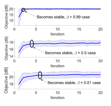
Convergence: Fig. 2 displays the convergence of the objective function/weighted SNR for different values of the weight of the radar SNR ($\beta$). The solid lines are the mean of objective of $50$ realizations, and the shaded areas around the mean show the variance of the different realizations. It is shown that the objective increases faster with larger $\beta$. Note that the radar SNR is quartic in $\mathbf{\Theta}$, and the communication SNR is quadratic in $\mathbf{\Theta}$, so the former is more sensitive to the change of $\mathbf{\Theta}$. Larger $\beta$, which means assigning the radar SNR more priority, will result in quicker increase of the weighted sum SNR/objective function. To well balance the radar and communication metrics, $\beta$ should be chosen such that $\beta\text{SNR}_{R}$ and $(1-\beta)\text{SNR}_{C}$ are on the same scale.

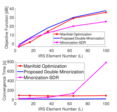
Comparisons with previous works: In Fig. 3, our proposed double minorization method is compared with minorization-SDR [13] and manifold optimization [17] when the number of IRS elements ($L$) changes. In [13], the quartic objective function is first surrogated with a quadratic one, then solved with SDR to obtain the covariance matrix of the IRS parameter. The IRS parameter is re-constructed from the covariance via Gaussian randomization. In [17], manifold optimization is proposed for the fourth order objective via Riemannian gradient ascent. Per the first subplot of Fig. 3, our proposed method outperforms [13] and [17], and the objective of weighted SNR is boosted by increasing $L$.

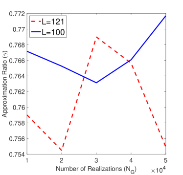
Remarks: The performance loss of [13] is obvious when $L$ is large. This comes from the Gaussian randomization operation, which computes the IRS parameter from its covariance. For the sake of simplicity and without loss of generality, we denote the optimal objective value of the SDP in the first step as $\mathrm{tr}\!\left[{\mathbf{A}\mathbf{R}_{\boldsymbol{\theta}}^{\ast}}\right]$, where ${\mathbf{R}_{\boldsymbol{\theta}}^{\ast}}$ is the optimal solution of ${\mathbf{R}_{\boldsymbol{\theta}}}$ which maximizes $\mathrm{tr}\!\left[{\mathbf{A}\mathbf{R}_{\boldsymbol{\theta}}}\right]$, and $\mathbf{R}_{\boldsymbol{\theta}}$ is the covariance matrix of $\boldsymbol{\theta}$. We realize $\boldsymbol{\xi}\sim\mathcal{CN}(\mathbf{0},\mathbf{R}_{\boldsymbol{\theta}}^{\ast})$ with $N_{G}$ samples, and choose the one that maximizes $\mathrm{tr}\!\left[{\mathbf{A}\boldsymbol{\xi}\boldsymbol{\xi}^{H}}\right]$, and we denote this solution as $\boldsymbol{\xi}^{\ast}$. The approximation ratio $\gamma=\mathrm{tr}\!\left[{\mathbf{A}\boldsymbol{\xi}^{\ast}(\boldsymbol{\xi}^{\ast})^{H}}\right]/\mathrm{tr}\!\left[{\mathbf{A}\mathbf{R}_{\boldsymbol{\theta}}^{\ast}}\right]$ is statistically increasing with the growth of $N_{G}$ [19]. However, as Fig. 4 shows, in large $N_{G}$ region, the ratio increases negligibly by increasing $N_{G}$ for large $L$. It is observed that, for [13], to obtain a high quality solution, we need to realize a large number of randomized solutions when $L$ is large.

References

- [1] A. Zhang, F. Liu, C. Masouros, R. W. Heath Jr. , Z. Feng, L. Zheng, and A. Petropulu, “An overview of signal processing techniques for joint communication and radar sensing,” accepted in IEEE Journal on Spetial Topics in Signal Processing (see also arXiv:2102.12780), 2021.
- [2] A. Hassanien, M. G. Amin, E. Aboutanios, and B. Himed, “Dual-function radar communication systems: A solution to the spectrum congestion problem,” IEEE Signal Processing Magazine, vol. 36, no. 5, pp. 115–126, sep 2019.
- [3] J. A. Zhang, M. L. Rahman, X. Huang, Y. J. Guo, S. Chen, and R. W. Heath, “Perceptive mobile network: Cellular networks with radio vision via joint communication and radar sensing,” IEEE Vehicular Technology Magazine, pp. 1–11, 2020.
- [4] F. Liu, L. Zheng, Y. Cui, C. Masouros, A. P. Petropulu, H. Griffiths, and Y. C. Eldar, “Seventy years of radar and communications: The road from separation to integration,” arXiv:2210.00446, 2022.
- [5] Z. Wei, F. Liu, C. Masouros, N. Su, and A. P. Petropulu, “Toward multi-functional 6G wireless networks: Integrating sensing, communication, and security,” IEEE Commun. Mag., vol. 60, no. 4, pp. 65–71, 2022.
- [6] F. Liu, C. Masouros, A. P. Petropulu, H. Griffiths, and L. Hanzo, “Joint radar and communication design: Applications, state-of-the-art, and the road ahead,” IEEE Transactions on Communications, vol. 68, no. 6, pp. 3834–3862, 2020.
- [7] D. Ma, N. Shlezinger, T. Huang, Y. Liu, and Y. C. Eldar, “Joint radar-communication strategies for autonomous vehicles: Combining two key automotive technologies,” IEEE Signal Processing Magazine, vol. 37, no. 4, pp. 85–97, 2020.
- [8] Q. Wu and R. Zhang, “Intelligent reflecting surface enhanced wireless network via joint active and passive beamforming,” IEEE Transactions on Wireless Communications, vol. 18, no. 11, pp. 5394–5409, 2019.
- [9] C. Huang, A. Zappone, G. C. Alexandropoulos, M. Debbah, and C. Yuen, “Reconfigurable intelligent surfaces for energy efficiency in wireless communication,” IEEE Trans. Wireless Commun., vol. 18, no. 8, pp. 4157–4170, 2019.
- [10] S. Buzzi, E. Grossi, M. Lops, and L. Venturino, “Foundations of MIMO radar detection aided by reconfigurable intelligent surfaces,” IEEE Trans. Signal Process., vol. 70, pp. 1749–1763, 2022.
- [11] F. Liu, L. Zhou, C. Masouros, A. Li, W. Luo, and A. Petropulu, “Toward dual-functional radar-communication systems: Optimal waveform design,” IEEE Trans. Signal Process., vol. 66, no. 16, pp. 4264–4279, 2018.
- [12] Y. Sun, P. Babu, and D. P. Palomar, “Majorization-minimization algorithms in signal processing, communications, and machine learning,” IEEE Trans. Signal Process., vol. 65, no. 3, pp. 794–816, 2017.
- [13] Z.-M. Jiang, M. Rihan, P. Zhang, L. Huang, Q. Deng, J. Zhang, and E. M. Mohamed, “Intelligent reflecting surface aided dual-function radar and communication system,” IEEE Syst. J., pp. 1–12, 2021.
- [14] R. Liu, M. Li, Y. Liu, Q. Wu, and Q. Liu, “Joint transmit waveform and passive beamforming design for RIS-aided DFRC systems,” IEEE J. Sel. Topics Signal Process., vol. 16, no. 5, pp. 995–1010, 2022.
- [15] H. Luo, R. Liu, M. Li, Y. Liu, and Q. Liu, “Joint beamforming design for RIS-assisted integrated sensing and communication systems,” IEEE Trans. Veh. Technol., pp. 1–5, 2022.
- [16] T. Wei, L. Wu, K. V. Mishra, and M. R. B. Shankar, “IRS-aided wideband dual-function radar-communications with quantized phase-shifts,” in 2022 IEEE 12th Sensor Array and Multichannel Signal Processing Workshop (SAM), 2022, pp. 465–469.
- [17] Y. Li and A. Petropulu, “Dual-function radar-communication system aided by intelligent reflecting surfaces,” in 2022 IEEE 12th Sensor Array and Multichannel Signal Processing Workshop (SAM), 2022, pp. 126–130.
- [18] M. Najafi, V. Jamali, R. Schober, and H. V. Poor, “Physics-based modeling and scalable optimization of large intelligent reflecting surfaces,” IEEE Trans. Commun., vol. 69, no. 4, pp. 2673–2691, 2021.
- [19] Z.-q. Luo, W.-k. Ma, A. M.-c. So, Y. Ye, and S. Zhang, “Semidefinite relaxation of quadratic optimization problems,” IEEE Signal Process. Mag., vol. 27, no. 3, pp. 20–34, 2010.
- [20] M. Grant and S. Boyd, “CVX: Matlab software for disciplined convex programming, version 2.1,” http://cvxr.com/cvx, Mar. 2014.
- [21] B. Li and A. P. Petropulu, “Joint transmit designs for coexistence of MIMO wireless communications and sparse sensing radars in clutter,” IEEE Trans. Aerosp. Electron. Syst., vol. 53, no. 6, pp. 2846–2864, 2017.
- [22] M. Soltanalian and P. Stoica, “Designing unimodular codes via quadratic optimization,” IEEE Trans. Signal Process., vol. 62, no. 5, pp. 1221–1234, 2014.
- [23] L. Wu, P. Babu, and D. P. Palomar, “Transmit waveform/receive filter design for MIMO radar with multiple waveform constraints,” IEEE Trans. Signal Process., vol. 66, no. 6, pp. 1526–1540, 2018.