Mining of Switching Sparse Networks for Missing Value Imputation in Multivariate Time Series

Kohei Obata SANKEN, Osaka UniversityOsakaJapan [email protected] , Koki Kawabata SANKEN, Osaka UniversityOsakaJapan [email protected] , Yasuko Matsubara SANKEN, Osaka UniversityOsakaJapan [email protected] and Yasushi Sakurai SANKEN, Osaka UniversityOsakaJapan [email protected]

(2024)

Abstract.

Multivariate time series data suffer from the problem of missing values, which hinders the application of many analytical methods. To achieve the accurate imputation of these missing values, exploiting inter-correlation by employing the relationships between sequences (i.e., a network) is as important as the use of temporal dependency, since a sequence normally correlates with other sequences. Moreover, exploiting an adequate network depending on time is also necessary since the network varies over time. However, in real-world scenarios, we normally know neither the network structure nor when the network changes beforehand. Here, we propose a missing value imputation method for multivariate time series, namely MissNet, that is designed to exploit temporal dependency with a state-space model and inter-correlation by switching sparse networks. The network encodes conditional independence between features, which helps us understand the important relationships for imputation visually. Our algorithm, which scales linearly with reference to the length of the data, alternatively infers networks and fills in missing values using the networks while discovering the switching of the networks. Extensive experiments demonstrate that MissNet outperforms the state-of-the-art algorithms for multivariate time series imputation and provides interpretable results.

Multivariate time series, Missing value imputation, Network inference, State-space model, Graphical lasso

^†^†journalyear: 2024^†^†copyright: acmlicensed^†^†conference: Proceedings of the 30th ACM SIGKDD Conference on Knowledge Discovery and Data Mining; August 25–29, 2024; Barcelona, Spain^†^†booktitle: Proceedings of the 30th ACM SIGKDD Conference on Knowledge Discovery and Data Mining (KDD ’24), August 25–29, 2024, Barcelona, Spain^†^†doi: 10.1145/3637528.3671760^†^†isbn: 979-8-4007-0490-1/24/08^†^†ccs: Information systems Data mining^†^†ccs: Mathematics of computing Time series analysis

1. Introduction

Refer to caption — Figure 1. An illustrative example of a multivariate time series including missing blocks, where each time point of the data is allocated to two regimes, each with a distinct network, where the edges show relationships between features.

With the development of the Internet of Things (IoT), multivariate time series are generated in many real-world applications, such as motion capture (Qin et al., 2020), and health monitoring (Chambon et al., 2018). However, there are inevitably many values missing from these data, and this has many possible causes (e.g., sensor malfunction). As most algorithms assume an intact input when building models, missing value imputation is indispensable for real-world applications (Shadbahr et al., 2023; Berrevoets et al., 2023).

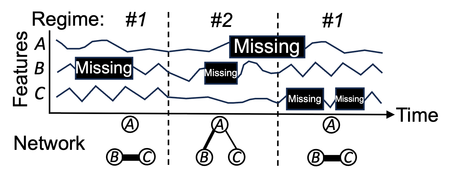
In time series data, missing values often occur consecutively, leading to a missing block in a sequence, and can happen simultaneously to multiple sequences (Liu et al., 2020). To effectively reconstruct missing values from such partially observed data, we must exploit both temporal dependency, by taking account of past and future values in the sequence, and inter-correlation, by using the relationship between different sequences (i.e., a network) (Cini et al., 2021; Yi et al., 2016). Here, a network does not necessarily mean the spatial proximity of sensors but rather underlying connectivity (e.g., Pearson correlation or partial correlation). Moreover, as time series data are normally non-stationary, so is the network; an adequate network must be exploited depending on time (Tomasi et al., 2018, 2021). We collectively refer to a group of time points with the same network as a “regime”. Fig. 1 shows an illustrative example where missing blocks randomly exist in a multivariate time series consisting of three features (i.e., A, B, and C). Each time point belongs to either of two regimes with different networks (i.e., $\#1$ and $\#2$ ), where the thickness of the edge indicates the strength of the interplay between features. It is appropriate to use the values of feature C to impute the block missing from feature B in regime $\#1$ since the network has an edge between B and C. On the other hand, in regime $\#2$ , it is preferable to use feature A, as the network suggests. Nevertheless, in real-world scenarios, we often have no information about the data; that is, we do not know the structure of the network, let alone when the network changes. Thus, given a partially observed multivariate time series, how can we infer networks and allocate each time point to the correct regime? How can we achieve an accurate imputation exploiting both temporal dependency and inter-correlation?

There have been many studies on time series missing value imputation with machine learning and deep learning models (Khayati et al., 2020). Many of them employ time-variant latent/hidden states, as used in a State-Space Model (SSM) or a Recurrent Neural Network (RNN), to learn the dynamic patterns of time series (Li et al., 2009; Chen and Sun, 2021; Cao et al., 2018; Yoon et al., 2018b). However, they do not make full use of inter-correlation, while the sequences of a multivariate time series usually interact. Although they implicitly capture inter-correlation in latent space, they potentially capture spurious correlations under the presence of missing values, leading to inaccurate imputation. To tackle this problem, several studies explicitly utilize the network (Cai et al., 2015a, b; Hairi et al., 2019; Jing et al., 2021; Cini et al., 2021; Wang et al., 2023a). However, they require a predefined network, even though we rarely know it in advance.

In this work, we propose MissNet ¹¹1Our source code and datasets are publicly available:
https://github.com/KoheiObata/MissNet. , Mining of switching sparse Networks for multivariate time series imputation, which repeatedly infers sparse networks from imputed data and fills in missing values using the networks while allocating each time point to regimes. Specifically, our model has three components: (1) a regime-switching model based on a discrete Markov process for detecting the change point of the network. (2) An imputation model based on an SSM for exploiting temporal dependency and inter-correlation by latent space and the networks. (3) A network inference model for inferring sparse networks via graphical lasso, where each network encodes pairwise conditional independencies among features, and the lasso penalty helps avoid capturing spurious correlations. Our proposed algorithm maximizes the joint probability distribution over the above components.

Our method has the following desired properties:

•

Effective: MissNet, which exploits both temporal dependency and inter-correlation by inferring switching sparse networks, outperforms the state-of-the-art algorithms for missing value imputation for multivariate time series.
•

Scalable: Our proposed algorithm scales linear with regard to the length of the time series and is thus applicable to a long-range time series.
•

Interpretable: MissNet discovers regimes with distinct sparse networks, which help us interpret data, e.g., what is the key relationship in the data, and why does a particular regime distinguish itself from others?

2. Related work

We review previous studies closely related to our work. Table 1 shows the relative advantages of MissNet. Current approaches fall short with respect to at least one of these desired characteristics.

Time series missing value imputation. Missing value imputation for time series is a very rich topic (Khayati et al., 2020). We roughly classify missing value imputation methods as Matrix Factorization (MF)-based, SSM-based, and Deep Learning (DL)-based approaches.

MF-based methods, such as SoftImpute (Mazumder et al., 2010) based on Singular Value Decomposition (SVD), recover missing values from low-dimensional embedding matrices of partially observed data (Papadimitriou et al., 2005; Khayati et al., 2014; Zhang and Balzano, 2016; Yi et al., 2016). For example, SoRec (Ma et al., 2008), proposed as a recommendation system, constrains MF with a predefined network to exploit inter-correlation. Since MF is limited in capturing temporal dependency, TRMF (Yu et al., 2016) uses an Auto-Regressive (AR) model and imposes temporal smoothness on MF.

SSMs, such as Linear Dynamical Systems (LDS) (Ghahramani, 1998), use latent space to capture temporal dependency, where the data point depends on all past data points (Rogers et al., 2013; Dabrowski et al., 2018; Chen and Sun, 2021; Hairi et al., 2019). To fit more complex time series, Switching LDS (SLDS) (Pavlovic et al., 1999; Fox et al., 2008) switches multiple LDS models. SSM-based methods, such as DynaMMo (Li et al., 2009), focus on capturing the dynamic patterns in time series rather than inter-correlation implicitly captured through the latent space. To use the underlying connectivity in multivariate time series, DCMF (Cai et al., 2015a), and its tensor extension Facets (Cai et al., 2015b) use SSM constrained with a predefined network, which is effective, especially when the missing rate is high. However, they assume that the network is accurately known and fixed, while it is usually unknown and may change over time in real-world scenarios.

Recently, extensive research has focused on DL-based methods, employing techniques including graph neural networks (Jing et al., 2021; Cini et al., 2021; Fan et al., 2023; Ren et al., 2023), self-attention (Shukla and Marlin, 2021; Du et al., 2023), and, most recently, diffusion models (Alcaraz and Strodthoff, 2022; Tashiro et al., 2021; Wang et al., 2023b), to harness their high model capacity (Yoon et al., 2018a; Bansal et al., 2021). For example, BRITS (Cao et al., 2018) and M-RNN (Yoon et al., 2018b) impute missing values according to hidden states from bidirectional RNN. To utilize dynamic inter-correlation in time series, POGEVON (Wang et al., 2023a) requires a sequence of networks and imputes missing values in time series and missing edges in the networks, assuming that the network varies over time. Although DL-based methods can handle complex data, the imputation quality depends heavily on the size and the selection of the training dataset.

Table 1. Capabilities of MissNet, Matrix Factorization (MF), State-Space Model (SSM), Deep Learning (DL), and Graphical Lasso (GL)-based approaches.

	MF			SSM			DL		GL
	SoftImpute (Mazumder et al., 2010)	SoRec (Ma et al., 2008)	TRMF (Yu et al., 2016)	SLDS (Pavlovic et al., 1999)	DynaMMo (Li et al., 2009)	DCMF (Cai et al., 2015a)	BRITS (Cao et al., 2018)	POGEVON (Wang et al., 2023a)	TICC (Hallac et al., 2017b)	MMGL (Tozzo et al., 2020)	MissNet
Temporal dependency	-	-	✓	✓	✓	✓	✓	✓	-	-	✓
Inter-correlation	-	✓	-	-	-	✓	-	✓	-	✓	✓
Time-varying inter-correlation	-	-	-	-	-	-	-	✓	-	✓	✓
Missing value imputation	✓	✓	✓	-	✓	✓	✓	✓	-	✓	✓
Segmentation	-	-	-	✓	-	-	-	-	✓	-	✓
Sparse network inference	-	-	-	-	-	-	-	-	✓	✓	✓

Sparse network inference. From another perspective, our method infers sparse networks from time series containing missing values and discovers regimes (i.e., clusters) based on networks. Inferring a sparse inverse covariance matrix (i.e., network) from data helps us to understand feature dependency in a statistical way. Graphical lasso (Friedman et al., 2008), which maximizes the Gaussian log-likelihood imposing an $\ell_{1}$ -norm penalty, is one of the most commonly used techniques for estimating a sparse network from static data. Städler and Bühlmann (Städler and Bühlmann, 2012a) have tackled inferring a sparse network from partially observed data according to conditional probability. However, the network varies over time (Namaki et al., 2011; Monti et al., 2014; Malte Londschien and Bühlmann, 2021); thus, TVGL (Hallac et al., 2017a) infers time-varying networks by considering the time similarity with a network belonging to neighboring segments. To infer time-varying networks in the presence of missing values, MMGL (Tozzo et al., 2020), which employs TVGL, uses the expectation-maximization (EM) algorithm to repeat the inference of time-varying networks and missing value imputation based on conditional probability under the condition that each segment has the same observed features. Discovering clusters based on networks (Obata et al., 2024), such as TICC (Hallac et al., 2017b) and TAGM (Tozzo et al., 2021), provides interpretable results that other traditional clustering methods cannot find. However, they cannot handle missing values.

As a consequence, none of the previous studies have addressed missing value imputation for multivariate time series by employing sparse network inference and segmentation based on the network.

3. Preliminaries

3.1. Problem definition

In this paper, we focus on the task of multivariate time series missing value imputation. We use a multivariate time series with $N$ features and $T$ timesteps $\bm{X}=\{\bm{x}_{1},\bm{x}_{2},\dots,\bm{x}_{T}\}\in\mathbb{R}^{N\times T}$ . To represent the missing values in $\bm{X}$ , we introduce the indicator matrix $\bm{W}\in\mathbb{R}^{N\times T}$ , where $\bm{W}_{i,t}$ indicates the availability of feature $i$ at timestep $t$ : $\bm{W}_{i,t}$ being $0$ or $1$ indicates whether $\bm{X}_{i,t}$ is missing or observed. Thus, the observed entries can be described as $\tilde{\bm{X}}=\bm{W}\circ\bm{X}$ , where $\circ$ is a Hadamard product. Our problem is formally written as follows:

Problem 1 (Multivariate Time Series Missing Value Imputation).

Given: a partially observed multivariate time series $\tilde{\bm{X}}$ ; Recover: its missing parts indicated by $\bm{W}$ .

3.2. Graphical lasso

We use graphical lasso (Friedman et al., 2008) to infer the network for each regime. Given $\bm{X}$ , graphical lasso estimates the sparse Gaussian inverse covariance matrix (i.e., network) $\bm{\Theta}\in\mathbb{R}^{N\times N}$ , also known as the precision matrix. The network encodes pairwise conditional independencies among $N$ features, e.g., if $\bm{\Theta}_{i,j}=0$ , then features $i$ and $j$ are conditionally independent given the values of all the other features. The optimization problem is expressed as follows:

(1)		$\displaystyle\textrm{minimize}_{\bm{\Theta}\in S^{p}_{++}}$	$\displaystyle\lambda\|\|\bm{\Theta}\|\|_{od,1}-\sum_{t=1}^{T}ll(\bm{x}_{t,},\bm{\Theta}),$
	$\displaystyle ll(\bm{x}_{t},\bm{\Theta})=$	$\displaystyle-\frac{1}{2}(\bm{x}_{t}-\bm{\rho})^{\prime}\bm{\Theta}(\bm{x}_{t}-\bm{\rho})$
(2)			$\displaystyle+\frac{1}{2}\log\textrm{det}(\bm{\Theta})-\frac{N}{2}\log(2\pi),$

where $\bm{\Theta}$ must be symmetric positive definite ( $S^{p}_{++}$ ). $ll(\bm{x}_{t},\bm{\Theta})$ is the log-likelihood and $\bm{\rho}\in\mathbb{R}^{N}$ is the empirical mean of $\bm{X}$ . $\lambda\geq 0$ is a hyperparameter for determining the sparsity level of the network, and $\|\cdot\|_{od,1}$ indicates the off-diagonal $\ell_{1}$ -norm. This is a convex optimization problem that can be solved via the alternating direction method of multipliers (ADMM) (Boyd et al., 2011).

4. Proposed MissNet

In this section, we present our proposed MissNet for missing value imputation. We give the formal formulation of the model and then provide the detailed algorithm to learn the model.

4.1. Optimization model

MissNet infers sparse networks and fills in missing values using the networks while discovering regimes. We first introduce three interacting components of our model: a regime-switching model, an imputation model, and a network inference model. Then, we define the optimization formulation.

Regime-switching model. MissNet describes the change of networks by regime-switching. Let $K$ be the number of regimes, $\bm{F}=\{\bm{f}_{1},\dots\bm{f}_{T}\}\in\mathbb{R}^{K\times T}$ be regime assignments, and $\bm{f}_{t}$ be a one-hot vector ²²2We use it interchangeably with the index of the regime (i.e., $\bm{f}_{t}^{th}$ -regime). that indicates $\tilde{\bm{x}}_{t}\in\mathbb{R}^{N}$ belongs to $\bm{f}_{t}^{th}$ -regime. We assume regime-switching to be a discrete first-order Markov process:

(3)

\displaystyle p(\bm{f}_{1})=\bm{\pi}_{0},\quad p(\bm{f}_{t+1}|\bm{f}_{t})=\bm{\Pi}_{\bm{f}_{t+1},\bm{f}_{t}},

where $\bm{\Pi}\in\mathbb{R}^{K\times K}$ is the Markov transition matrix and $\bm{\pi}_{0}\in\mathbb{R}^{K}$ is the initial state distribution.

Imputation model. MissNet imputes missing values exploiting temporal dependency and inter-correlation indicated by the networks. We assume that the temporal dependency is consistent throughout all regimes and captured in the latent space of an SSM, which allows us to consider long-term dependency. We define the latent states $\bm{Z}=\{\bm{z}_{1},\bm{z}_{2},\dots,\bm{z}_{T}\}\in\mathbb{R}^{L\times T}$ corresponding to $\tilde{\bm{X}}$ , where $L$ is the number of latent dimensions, and $\bm{z}_{t+1}\in\mathbb{R}^{L}$ is linear to $\bm{z}_{t}$ through the transition matrix $\bm{B}\in\mathbb{R}^{L\times L}$ with the covariance $\bm{\Sigma}_{\bm{Z}}$ , shown in Eq. (5). As defined in Eq. (4), the first timestep of latent state $\bm{z}_{1}$ is defined by the initial state $\bm{z}_{0}$ and the covariance $\bm{\Psi}_{0}$ .

(4)		$\displaystyle\bm{z}_{1}\sim$	$\displaystyle\mathcal{N}(\bm{z}_{0},\bm{\Psi}_{0}),$
(5)		$\displaystyle\bm{z}_{t+1}\|\bm{z}_{t}\sim$	$\displaystyle\mathcal{N}(\bm{B}\bm{z}_{t},\bm{\Sigma}_{\bm{Z}}).$

We define the observation $\tilde{\bm{x}}_{t}$ assigned to $\bm{f}_{t}^{th}$ -regime as being linear to the latent state $\bm{z}_{t}$ through the observation matrix of $\bm{f}_{t}^{th}$ -regime $\bm{U}^{(\bm{f}_{t})}\in\mathbb{R}^{N\times L}$ with the covariance $\bm{\Sigma}_{\bm{X}^{(\bm{f}_{t})}}$ :

(6)

\displaystyle\tilde{\bm{x}}_{t}|\bm{z}_{t},\bm{U}^{(\bm{f}_{t})},\bm{f}_{t}

\displaystyle\sim\mathcal{N}(\bm{U}^{(\bm{f}_{t})}\bm{z}_{t},\bm{\Sigma}_{\bm{X}^{(\bm{f}_{t})}}).

MissNet captures inter-correlation by adding a constraint on $\bm{U}^{(k)}$ . Let it be assumed that the contextual matrix of the $k^{th}$ -regime $\bm{S}^{(k)}\in\mathbb{R}^{N\times N}$ encodes the inter-correlation of $\bm{X}$ belonging to the $k^{th}$ -regime ( $1\leq k\leq K$ ). We define the contextual latent factor of the $k^{th}$ -regime $\bm{V}^{(k)}\in\mathbb{R}^{L\times N}$ , and the $j$ -th column ( $1\leq j\leq N$ ) of the contextual matrix $\bm{s}^{(k)}_{j}$ as linear to $\bm{v}^{(k)}_{j}$ through the observation matrix $\bm{U}^{(k)}$ with the covariance $\bm{\Sigma}_{\bm{S}^{(k)}}$ , formulated in Eq. (7). In Eq. (8), we place zero-mean spherical Gaussian priors on $\bm{v}^{(k)}_{j}$ under the assumption that $-1\leq\bm{S}^{(k)}_{i,j}\leq 1$ .

(7)		$\displaystyle\bm{s}^{(k)}_{j}\|\bm{v}^{(k)}_{j},\bm{U}^{(k)}$	$\displaystyle\sim\mathcal{N}(\bm{U}^{(k)}\bm{v}^{(k)}_{j},\bm{\Sigma}_{\bm{S}^{(k)}}),$
(8)		$\displaystyle\bm{v}^{(k)}_{j}$	$\displaystyle\sim\mathcal{N}(0,\bm{\Sigma}_{\bm{V}^{(k)}}).$

To avoid our model overfitting the observed entries since many entries are missing, we simplify the covariances by assuming that all noises are independent and identically distributed (i.i.d.). Thus, the parameters $\bm{\Sigma}_{\bm{Z}},\bm{\Sigma}_{\bm{X}^{(k)}},\bm{\Sigma}_{\bm{S}^{(k)}},\bm{\Sigma}_{\bm{V}^{(k)}}$ are reduced to $\sigma_{\bm{Z}}^{2},\sigma_{\bm{X}^{(k)}}^{2},\sigma_{\bm{S}^{(k)}}^{2},\linebreak\sigma_{\bm{V}^{(k)}}^{2}$ , respectively (i.e., $\bm{\Sigma}_{\bm{Z}}=\sigma_{\bm{Z}}^{2}\bm{I}$ , $\bm{\Sigma}_{\bm{X}^{(k)}}=\sigma_{\bm{X}^{(k)}}^{2}\bm{I}$ , $\bm{\Sigma}_{\bm{S}^{(k)}}=\sigma_{\bm{S}^{(k)}}^{2}\bm{I}$ , and $\bm{\Sigma}_{\bm{V}^{(k)}}=\sigma_{\bm{V}^{(k)}}^{2}\bm{I}$ ).

With the above imputation model, the imputed time series $\hat{\bm{x}}_{t}$ at timestep $t$ is recovered as follows:

(9)

\displaystyle\hat{\bm{x}}_{t}=\bm{W}_{:,t}\circ\tilde{\bm{x}}_{t}+(1-\bm{W}_{:,t})\circ\bm{U}^{(\bm{f}_{t})}\bm{z}_{t}.

Network inference model. MissNet infers the network for each regime to exploit inter-correlation. We define a Gaussian distribution and $\ell_{1}$ -norm for the imputed data belonging to each regime to allow us to estimate networks accurately:

(10)

\displaystyle\hat{\bm{x}}_{t}|\bm{f}_{t}\sim\mathcal{N}(\bm{\rho}^{(\bm{f}_{t})},\bm{\Theta}^{(\bm{f}_{t})-1}),\>\>\>s.t.,||\bm{\Theta}^{(\bm{f}_{t})}||_{od,1}\leq\frac{e}{\lambda},

where $e$ is any constant value for convenience, and $\lambda$ is a hyperparameter that controls the sparsity of the network (i.e., inverse covariance matrix) $\bm{\Theta}^{(\bm{f}_{t})}$ with $\ell_{1}$ -norm, which helps avoid capturing spurious correlations.

Optimazation formulation. Our goal is to estimate the model parameters $\theta=\{\bm{B},\bm{z}_{0},\bm{\Psi}_{0},\sigma_{\bm{Z}},\dot{\sigma_{\bm{X}}},\dot{\sigma_{\bm{S}}},\dot{\sigma_{\bm{V}}},\dot{\bm{\rho}},\dot{\bm{\Theta}},\bm{\pi}_{0},\bm{\Pi}\}$ and find the latent factors $\bm{Z},\dot{\bm{V}},\dot{\bm{U}},\dot{\bm{S}},\bm{F}$ , where the letters with a dot indicate a set of $K$ vectors/matrices/scalers (e.g., $\dot{\bm{S}}=\{\bm{S}^{(k)}\}_{k=1}^{K}$ ), that maximizes the following joint probability distribution:

	$\displaystyle\mathop{\rm arg~{}max}\limits p(\tilde{\bm{X}},\bm{Z},\dot{\bm{V}},\dot{\bm{U}},\dot{\bm{S}},\bm{F})=\underbrace{p(\bm{z}_{1})\prod_{t=2}^{T}p(\bm{z}_{t}\|\bm{z}_{t-1})}_{\text{temporal dependency}}$
	$\displaystyle\underbrace{\prod_{t=1}^{T}p(\tilde{\bm{x}}_{t}\|\bm{z}_{t-1},\bm{U}^{(\bm{f}_{t})},\bm{f}_{t})}_{\text{time series}}\underbrace{\prod_{k=1}^{K}\Bigg{\{}\prod_{j=1}^{N}p(\bm{v}^{(k)}_{j})\prod_{j=1}^{N}p(\bm{s}^{(k)}_{j}\|\bm{U}^{(k)},\bm{v}^{(k)}_{j})\Bigg{\}}}_{\text{network constraint}}$
	$\displaystyle\underbrace{p(\bm{f}_{1})\prod_{t=2}^{T}p(\bm{f}_{t}\|\bm{f}_{t-1})}_{\text{regime-switching}}\underbrace{\prod_{t=1}^{T}p(\hat{\bm{x}}_{t}\|\bm{\rho}^{(\bm{f}_{t})},\bm{\Theta}^{(\bm{f}_{t})},\bm{f}_{t})}_{\text{network inference}},\quad\underbrace{(s.t.\|\|\bm{\Theta}^{(k)}\|\|_{od,1}\leq\frac{e}{\lambda})}_{\text{network sparsity}}.$

4.2. Algorithm

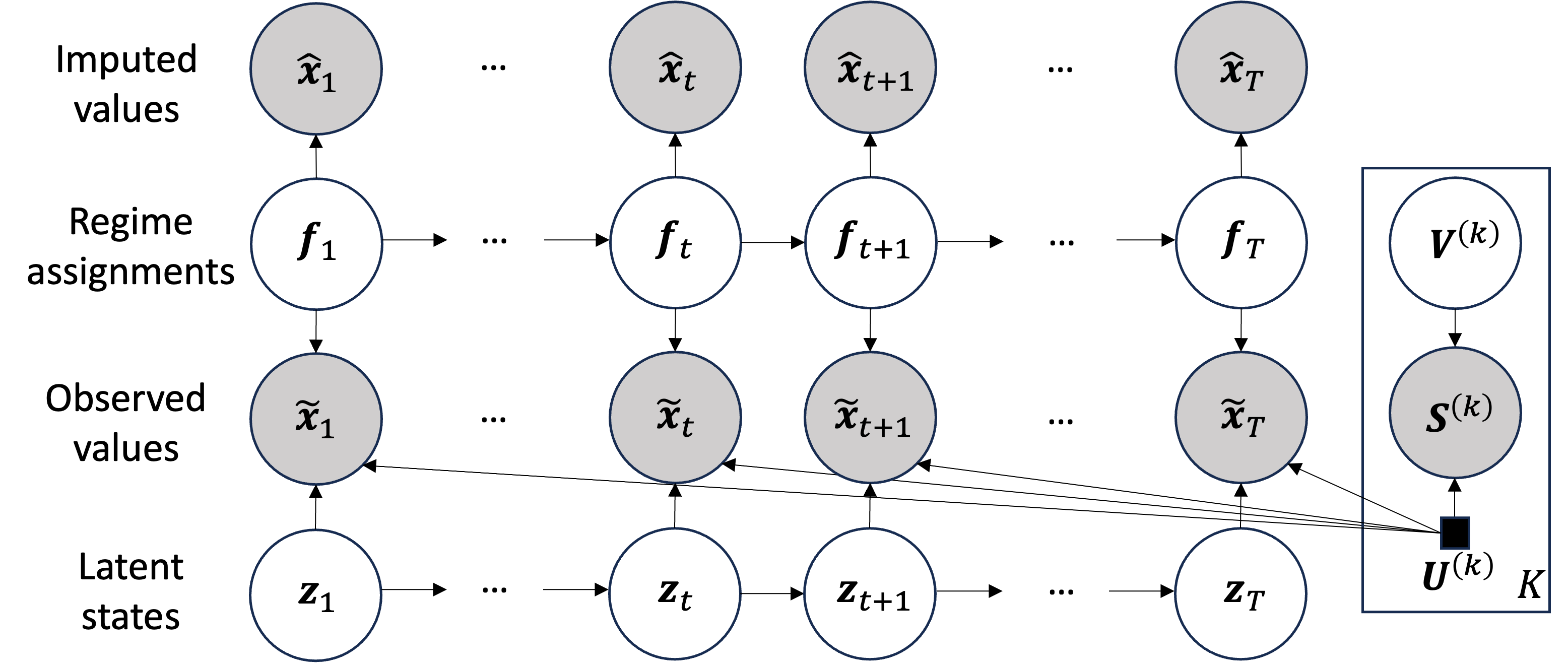
It is difficult to find the global optimal solution of Eq. (4.1), for the following reasons: $\mathrm{(\hskip 1.79993pti\hskip 1.79993pt)}$ As a constraint for $\dot{\bm{U}}$ , $\dot{\bm{S}}$ has to be fixed and encode inter-correlation; $\mathrm{(\hskip 0.80002ptii\hskip 0.80002pt)}$ $\dot{\bm{U}}$ , $\bm{Z}$ and $\bm{F}$ jointly determine $\tilde{\bm{X}}$ , and $\dot{\bm{U}}$ and $\dot{\bm{V}}$ jointly determine $\dot{\bm{S}}$ ; $\mathrm{(iii)}$ Calculating the correct $\bm{F}$ is NP-hard. Hence, we aim to find its local optimum instead, following the EM algorithm, where the graphical model for each iteration is shown in Fig. 2. Specifically, to address the aforementioned difficulties, we employ the following steps: $\mathrm{(\hskip 1.79993pti\hskip 1.79993pt)}$ we consider $\dot{\bm{S}}$ is observed in each iteration, and we update it at the end of the iteration using $\dot{\bm{\Theta}}$ ; $\mathrm{(\hskip 0.80002ptii\hskip 0.80002pt)}$ we regard $\dot{\bm{U}}$ as a model parameter, thus $\{\tilde{\bm{X}},\bm{Z},\bm{F}\}$ are independent with $\{\dot{\bm{S}},\dot{\bm{V}}\}$ . We alternate the inference of $\{\bm{Z},\bm{F}\}$ and $\dot{\bm{V}}$ and the update of the model parameters; $\mathrm{(iii)}$ we employ a Viterbi approximation and infer the most likely $\bm{F}$ .

4.2.1. E-step

Given $\dot{\bm{U}}$ , we can infer $\{\bm{Z},\bm{F}\}$ and $\dot{\bm{V}}$ independently.

Let $\bm{o}_{t}$ denote the indices of the observed entries of $\tilde{\bm{x}}_{t}$ . The observed-only data $\bar{\bm{x}}_{t}$ and the corresponding observed-only observation matrix $\bar{\bm{U}}^{(k)}_{t}$ are defined as follows:

	$\displaystyle\bm{o}_{t}=\{i\|\bm{W}_{i,t}>0,i=1,\dots,N\},$
(12)		$\displaystyle\bar{\bm{x}}_{t}=\tilde{\bm{x}}_{t}(\bm{o}_{t}),\quad\bar{\bm{U}}^{(k)}_{t}=\bm{U}^{(k)}(\bm{o}_{t},:).$

Inferring $\bm{F}$ and $\bm{Z}$ . $\bm{F}$ and $\bm{Z}$ are coupled, and so must be jointly determined. We first use a Viterbi approximation to find the most likely regime assignments $\bm{F}$ that maximize the log-likelihood Eq. (4.1). The likelihood term obtained during the calculation of $\bm{F}$ also acts as a Kalman Filter (forward algorithm). Then, we infer $\bm{Z}$ with a Rauch-Tung-Streibel (RTS) smoother (backward algorithm).

In a Viterbi approximation, finding $\bm{F}$ requires the partial cost $J_{t,t-1,k,l}$ when the switch is to regime $k$ at time $t$ from regime $l$ at time $t-1$ . To calculate the partial cost, we define the following LDS state and variance terms:

	$\displaystyle\bm{\mu}_{t\|t-1,k,l}$	$\displaystyle=\bm{B}\bm{\mu}_{t-1\|t-1,k,l},$
	$\displaystyle\bm{\mu}_{t\|t,k,l}$	$\displaystyle=\bm{\mu}_{t\|t-1,k,l}+\bm{D}_{t,k,l}(\bar{\bm{x}}_{t}-\bar{\bm{U}}^{(k)}_{t}\bm{B}\bm{\mu}_{t\|t-1,k,l}),$
	$\displaystyle\bm{\Psi}_{t\|t-1,k,l}$	$\displaystyle=\bm{B}\bm{\Psi}_{t-1\|t-1,k,l}\bm{B}^{\prime}+\sigma_{\bm{Z}}^{2}\bm{I},$
	$\displaystyle\bm{\Psi}_{t\|t,k,l}$	$\displaystyle=(\bm{I}-\bm{D}_{t,k,l}\bar{\bm{U}}^{(k)}_{t})\bm{\Psi}_{t-1\|t-1,k,l},$
(13)		$\displaystyle\bm{D}_{t,k,l}$	$\displaystyle=\bm{\Psi}_{t\|t-1,k,l}\bar{\bm{U}}^{(k)^{\prime}}_{t}(\bar{\bm{U}}^{(k)}_{t}\bm{\Psi}_{t\|t-1,k,l}\bar{\bm{U}}^{(k)^{\prime}}_{t}+\sigma_{\bm{X}^{(k)}}^{2}\bm{I})^{-1},$

with the initial state:

	$\displaystyle\bm{\mu}_{1\|1,k}$	$\displaystyle=\bm{z}_{0}+\bm{D}_{1,k}(\bar{\bm{x}}_{1}-\bar{\bm{U}}^{(k)}_{1}\bm{z}_{0}),$
	$\displaystyle\bm{\Psi}_{1\|1,k}$	$\displaystyle=(\bm{I}-\bm{D}_{1,k}\bar{\bm{U}}^{(k)}_{1})\bm{\Psi}_{0},$
(14)		$\displaystyle\bm{D}_{1,k}$	$\displaystyle=\bm{\Psi}_{0}\bar{\bm{U}}^{(k)^{\prime}}_{1}(\bar{\bm{U}}^{(k)}_{1}\bm{\Psi}_{0}\bar{\bm{U}}^{(k)^{\prime}}_{1}+\sigma_{\bm{X}^{(k)}}^{2}\bm{I})^{-1},$

where $\bm{\mu}_{t|t-1,k,l}$ and $\bm{\mu}_{t|t,k,l}$ are the one-step predicted LDS state and the best-filtered state estimates at $t$ , respectively, given the switch is in regime $k$ at time $t$ and in regime $l$ at time $t-1$ and only the $t-1$ measurements are known. Similar definitions are used for $\bm{\Psi}_{t|t-1,k,l}$ and $\bm{\Psi}_{t|t,k,l}$ .

The partial cost is obtained by calculating the logarithm of Eq. (4.1) related to $\bm{f}_{t}$ :

	$\displaystyle J_{t,t-1,k,l}=$	$\displaystyle\frac{1}{2}(\bar{\bm{x}}_{t}-\bar{\bm{U}}^{(k)}_{t}\bm{\mu}_{t\|t-1,k,l})^{\prime}\bm{R}(\bar{\bm{x}}_{t}-\bar{\bm{U}}^{(k)}_{t}\bm{\mu}_{t\|t-1,k,l})$
		$\displaystyle-\frac{1}{2}\log\textrm{det}(\bm{R})+\frac{L}{2}log(2\pi)$
		$\displaystyle+\frac{1}{2}(\hat{\bm{x}}_{t}-\bm{\rho}^{(k)})^{\prime}\bm{\Theta}^{(k)}(\hat{\bm{x}}_{t}-\bm{\rho}^{(k)})$
(15)			$\displaystyle-\frac{1}{2}\log\textrm{det}(\bm{\Theta}^{(k)})+\frac{N}{2}\log(2\pi)-\log(\bm{\Pi}_{k,l}),$
	$\displaystyle\bm{R}=$	$\displaystyle(\bar{\bm{U}}^{(k)}_{t}\bm{\Psi}_{t\|t-1,k,l}\bar{\bm{U}}^{(k)^{\prime}}_{t}+\sigma_{\bm{X}^{(k)}}^{2}\bm{I})^{-1}.$

Once all partial costs are obtained, it is well-known how to apply a Viterbi inference to a discrete Markov process to obtain the most likely regime assignments $\bm{F}$ (Viterbi, 1967).

Then, we infer $\bm{Z}$ . Let the posteriors of $\bm{z}_{t}$ be as follows:

	$\displaystyle p(\bm{z}_{t}\|\tilde{\bm{x}}_{1},\dots,\tilde{\bm{x}}_{t})=\mathcal{N}(\bm{z}_{t}\|\bm{\mu}_{t},\bm{\Psi}_{t}),$
(16)		$\displaystyle p(\bm{z}_{t}\|\tilde{\bm{x}}_{1},\dots,\tilde{\bm{x}}_{T})=\mathcal{N}(\bm{z}_{t}\|\bm{\hat{\mu}}_{t},\bm{\hat{\Psi}}_{t}).$

We now obtain $\bm{\mu}_{t},\bm{\Psi}_{t},\bm{\Psi}_{t|t-1}$ using $\bm{F}$ ; thus, in practice, we have conducted a Kalman Filter. We apply the RTS smoother to infer $\bm{Z}$ .

	$\displaystyle\bm{\hat{\mu}}_{t}$	$\displaystyle=\bm{\mu}_{t}+\bm{C}_{t}(\bm{\hat{\mu}}_{t+1}-\bm{B}\bm{\mu}_{t}),$
	$\displaystyle\bm{\hat{\Psi}}_{t}$	$\displaystyle=\bm{\Psi}_{t}+\bm{C}_{t}(\bm{\hat{\Psi}}_{t+1}-\bm{\Psi}_{t\|t-1})\bm{C}^{\prime}_{t},$
(17)		$\displaystyle\bm{C}_{t}$	$\displaystyle=\bm{\Psi}_{t}\bm{B}^{\prime}(\bm{\Psi}_{t\|t-1})^{-1},$
	$\displaystyle\mathbb{E}[\bm{z}_{t}]$	$\displaystyle=\bm{\hat{\mu}}_{t},$
	$\displaystyle\mathbb{E}[\bm{z}_{t}\bm{z}^{\prime}_{t-1}]$	$\displaystyle=\bm{\hat{\Psi}}_{t}\bm{C}^{\prime}_{t}+\bm{\hat{\mu}}_{t}\bm{\hat{\mu}}^{\prime}_{t-1},$
(18)		$\displaystyle\mathbb{E}[\bm{z}_{t}\bm{z}^{\prime}_{t}]$	$\displaystyle=\bm{\hat{\Psi}}_{t}+\bm{\hat{\mu}}_{t}\bm{\hat{\mu}}^{\prime}_{t-1}.$

Inferring $\dot{\bm{V}}$ . We apply Bayes’ theorem to Eq. (7) and (8) to obtain the posteriors $p(\bm{v}^{(k)}_{j}|\bm{s}^{(k)}_{j})=\mathcal{N}(\bm{v}^{(k)}_{j}|\bm{\nu}^{(k)}_{j},\bm{\Upsilon}^{(k)})$ :

	$\displaystyle\bm{\nu}^{(k)}_{j}$	$\displaystyle=\bm{M}^{(k)-1}\bm{U}^{(k)^{\prime}}\bm{s}^{(k)}_{j},$
	$\displaystyle\bm{\Upsilon}^{(k)}$	$\displaystyle=\sigma_{\bm{S}^{(k)}}^{2}\bm{M}^{(k)-1},$
	$\displaystyle\bm{M}^{(k)}$	$\displaystyle=\bm{U}^{(k)^{\prime}}\bm{U}^{(k)}+\sigma_{\bm{V}^{(k)}}^{-2}\sigma_{\bm{S}^{(k)}}^{2}\bm{I},$
	$\displaystyle\mathbb{E}[\bm{v}^{(k)}_{j}]$	$\displaystyle=\bm{\nu}^{(k)}_{j},$
(19)		$\displaystyle\mathbb{E}[\bm{v}^{(k)}_{j}\bm{v}^{(k)^{\prime}}_{j}]$	$\displaystyle=\bm{\Upsilon}^{(k)}+\bm{\nu}^{(k)}_{j}\bm{\nu}^{(k)^{\prime}}_{j}.$

4.2.2. M-step

After obtaining $\{\bm{Z},\bm{F}\}$ and $\dot{\bm{V}}$ , we update the model parameters to maximize the expectation of the log-likelihood:

(20)		$\displaystyle\theta^{new}$	$\displaystyle=\mathop{\rm arg~{}max}\limits_{\theta}Q(\theta,\theta^{old}),$
	$\displaystyle Q(\theta,\theta^{old})$	$\displaystyle=\mathbb{E}_{\bm{Z},\bm{F},\dot{\bm{V}}\|\theta^{old}}[\log p(\tilde{\bm{X}},\bm{Z},\dot{\bm{V}},\dot{\bm{U}},\dot{\bm{S}},\bm{F}\|\theta)]-\sum_{k=1}^{K}\lambda\|\|\bm{\Theta}^{(k)}\|\|_{od,1},$

where we incorporate the $\ell_{1}$ -norm constraint.

Parameters for the imputation model, $\dot{\bm{U}}$ and $\{\bm{B},\bm{z}_{0},\bm{\Psi}_{0},\sigma_{\bm{Z}},\dot{\sigma_{\bm{X}}},\dot{\sigma_{\bm{S}}},\dot{\sigma_{\bm{V}}}\}$ , can be obtained by taking the derivative of $Q(\theta,\theta^{old})$ . For $\bm{U}^{(k)}$ , we update each row $\bm{U}^{(k)}_{i,:}$ individually:

(21)		$\displaystyle(\bm{U}^{(k)}_{i,:})^{new}$	$\displaystyle=\bm{A_{1}}^{(k)}\bm{A_{2}}^{(k)-1},$
	$\displaystyle\bm{A_{1}}^{(k)}=\alpha\sigma_{\bm{S}^{(k)}}^{-2}\sum_{j=1}^{N}\bm{S}^{(k)}_{i,j}\mathbb{E}[\bm{v}^{(k)^{\prime}}_{j}]$	$\displaystyle+(1-\alpha)\sigma_{\bm{X}^{(k)}}^{-2}\sum_{t=1,\bm{f}_{t}\in k}^{T}\bm{W}_{i,t}\tilde{\bm{X}}_{i,t}\mathbb{E}[\bm{z}^{\prime}_{t}],$
	$\displaystyle\bm{A_{2}}^{(k)}=\alpha\sigma_{\bm{S}^{(k)}}^{-2}\sum_{j=1}^{N}\mathbb{E}[\bm{v}^{(k)}_{j}\bm{v}^{(k)^{\prime}}_{j}]$	$\displaystyle+(1-\alpha)\sigma_{\bm{X}^{(k)}}^{-2}\sum_{t=1,\bm{f}_{t}\in k}^{T}\bm{W}_{i,t}\mathbb{E}[\bm{z}_{t}\bm{z}^{\prime}_{t}],$

where $0\leq\alpha\leq 1$ is a hyperparameter employed as a trade-off for the contributions of inter-correlation and temporal dependency. The details of updating $\{\bm{B},\bm{z}_{0},\bm{\Psi}_{0},\sigma_{\bm{Z}},\dot{\sigma_{\bm{X}}},\dot{\sigma_{\bm{S}}},\dot{\sigma_{\bm{V}}}\}$ are presented in Appendix A.3.

For the network inference model, we calculate $\hat{\bm{X}}$ with Eq. (22) and then update $\bm{\rho}^{(k)}$ by calculating the empirical mean of $\hat{\bm{X}}$ belonging to the $k^{th}$ -regime and $\bm{\Theta}^{(k)}$ by solving the graphical lasso problem shown in Eq. (23) via ADMM.

(22)		$\displaystyle\hat{\bm{x}}_{t}=\bm{W}_{:,t}\circ\tilde{\bm{x}}_{t}+(1-\bm{W}_{:,t})\circ(\bm{U}^{(\bm{f}_{t})})^{new}\bm{\hat{\mu}}_{t},$
(23)		$\displaystyle\textrm{minimize}_{\bm{\Theta}^{(k)}\in S^{p}_{++}}\lambda\|\|\bm{\Theta}^{(k)}\|\|_{od,1}-\sum_{t=1,\bm{f}_{t}\in k}^{T}ll(\hat{\bm{x}}_{t},\bm{\Theta}^{(k)}).$

For the regime-switching model, the initial state distribution and the Markov transition matrix are updated as follows:

(24)

\displaystyle\bm{\pi}_{0}=\bm{f}_{1},\quad\bm{\Pi}=\bigg{(}\sum_{t=2}^{T}\bm{f}_{t}\bm{f}_{t-1}^{\prime}\bigg{)}\textrm{diag}\bigg{(}\sum_{t=2}^{T}\bm{f}_{t}\bigg{)}^{-1}.

4.2.3. Update $\dot{\bm{S}}$

We update $\bm{S}^{(k)}$ at the end of each iteration. As shown in Eq. (25), we define the off-diagonal elements of $\bm{S}^{(k)}$ as partial correlations calculated from the network $\bm{\Theta}^{(k)}$ to encode the inter-correlation.

(25)

\displaystyle\bm{S}^{(k)}_{i,j}

\displaystyle=\begin{cases}1&(i=j)\\ -(\frac{\bm{\Theta}^{(k)}_{i,j}}{\sqrt{\bm{\Theta}^{(k)}_{i,i}}\sqrt{\bm{\Theta}^{(k)}_{j,j}}})&(i\neq j)\end{cases}.

Algorithm 1 MissNet (

\tilde{\bm{X}},\bm{W},L,K,\alpha,\lambda

)

1: Input: (a) partially observed multivariate time series

\tilde{\bm{X}}

, (b) indicator matrix

\bm{W}

, (c) and hyperparameters

L,K,\alpha,\lambda

2: Output: latent factors

\bm{Z},\dot{\bm{V}},\dot{\bm{U}},\dot{\bm{S}},\bm{F}

model parameters

\theta

, and

\hat{\bm{X}}

3: Initialize

\hat{\bm{X}}

with linear interpolation,

\bm{Z},\dot{\bm{V}},\dot{\bm{U}},\dot{\bm{S}},\bm{F}

, and

\theta

;

4: repeat

5: for

t=1:T

6: for

k=1:K

7: for

l=1:K

8: Calculate partial cost

J_{t,t-1,k,l}

using Eq. (15)

9: end for

10: end for

11: end for

12: Infer

\bm{F}

and obtain

\bm{\mu}_{t},\bm{\Psi}_{t}

based on Eq. (13), (14)

13: for

t=T:1

14: Infer

\bm{\hat{\mu}}_{t},\bm{\hat{\Psi}}_{t},\mathbb{E}[\bm{z}_{t}\bm{z}^{\prime}_{t-1}],\mathbb{E}[\bm{z}_{t}\bm{z}^{\prime}_{t}]

by Eq. (17), (18)

15: end for

16: for

j=1:N

17: Infer

\mathbb{E}[\bm{v}^{(k)}_{j}],\mathbb{E}[\bm{v}^{(k)}_{j}\bm{v}^{(k)^{\prime}}_{j}]

using Eq. (19)

18: end for

19: Set

\bm{Z}=\{\bm{\hat{\mu}}_{1},\dots,\bm{\hat{\mu}}_{T}\}

\{\bm{V}^{(k)}=\{\bm{\nu}^{(k)}_{1},\dots,\bm{\nu}^{(k)}_{N}\}\}_{k=1}^{K}

20: Update

\dot{\bm{U}}

\theta

and

\hat{\bm{X}}

by Eq. (21) - (24)

21: Update

\dot{\bm{S}}

based on Eq. (25)

22: until convergence;

23: return

\{\bm{Z},\dot{\bm{V}},\dot{\bm{U}},\dot{\bm{S}},\bm{F},\theta,\hat{\bm{X}}\}

;

4.2.4. Overall algorithm

We have the overall algorithm shown as Alg. 1 to obtain a local optimal solution of Eq. (4.1). Given a partially observed multivariate time series $\tilde{\bm{X}}$ , an indicator matrix $\bm{W}$ , the dimension of latent state $L$ , the number of regimes $K$ , the network parameter $\alpha$ , and the sparse parameter $\lambda$ , our algorithm aims to find the latent factors $\bm{Z},\dot{\bm{V}},\dot{\bm{U}},\dot{\bm{S}},\bm{F}$ , other model parameters in $\theta$ , and imputed time series $\hat{\bm{X}}$ .

The MissNet algorithm starts by initializing $\hat{\bm{X}}$ with a linear interpolation, and by randomly initializing $\bm{Z},\dot{\bm{V}},\dot{\bm{U}},\dot{\bm{S}},\bm{F}$ , and $\theta$ (Line 3). Then, it alternately updates the latent factors and parameters until they converge. In each iteration, we consider $\dot{\bm{S}}$ to be given and $\dot{\bm{U}}$ to be a model parameter. In an iteration, we first conduct a Viterbi approximation to calculate the most likely regime assignments $\bm{F}$ (Line 5-12). Then, we infer the expectations of $\bm{Z}$ and $\dot{\bm{V}}$ (Line 13-15 and Line 16-18), and we update $\dot{\bm{U}}$ and model parameters $\theta$ (Line 20), and at the end of the iteration, we update $\dot{\bm{S}}$ (Line 21).

4.3. Complexity analysis

Lemma 0.

The time complexity of MissNet is
$O(\#iter\cdot(K^{2}\sum_{t=1}^{T}(L^{3}+L^{2}N_{t}+LN_{t}^{2}+N_{t}^{3})+KL^{2}N^{2}+KTL^{2}N+KN^{3}))$ .

Proof.

See Appendix A.2. ∎

$N_{t}$ represents the number of observed features of $\bar{\bm{x}}_{t}$ . Note that $K^{2}\sum_{t=1}^{T}(L^{3}+L^{2}N_{t}+LN_{t}^{2}+N_{t}^{3})$ is upper bounded by $K^{2}TN^{3}$ . In practice, the length of the time series ( $T$ ) is often orders of magnitude greater than the number of features ( $N$ ). Hence, the actual running time of MissNet is dominated by the term related to $T$ , which is linear in $T$ .

Lemma 0.

The space complexity of MissNet is
$O(TN+K^{2}TL^{2}+KL^{2}N+KN^{2})$ .

Proof.

See Appendix A.2. ∎

5. Experiments

In this section, we empirically evaluate our approach against state-of-the-art baselines on 12 datasets. We present experimental results for the following questions:
Q1. Effectiveness: How accurate is the proposed MissNet for recovering missing values?
Q2. Scalability: How does the proposed algorithm scale?
Q3. Interpretability: How can MissNet help us understand the data?

5.1. Experimental setup

5.1.1. Datasets

We use the following datasets.

Synthetic. We generate two types of synthetic data, PatternA and PatternB, five times each, by defining $\bm{Z}$ and $\dot{\bm{U}}$ . We set $T=1000,N=50$ and $L=10$ (Appendix B.1). PatternA has one regime ( $K=1$ ), and in PatternB ( $K=2$ ), two regimes switch at every $200$ timesteps.

MotionCapture. This dataset contains nine types of full body motions of MotionCapture database ³³3http://mocap.cs.cmu.edu. Each motion measures the positions of $41$ bones in the human body, resulting in a total of $123$ features (X, Y, and Z coordinates).

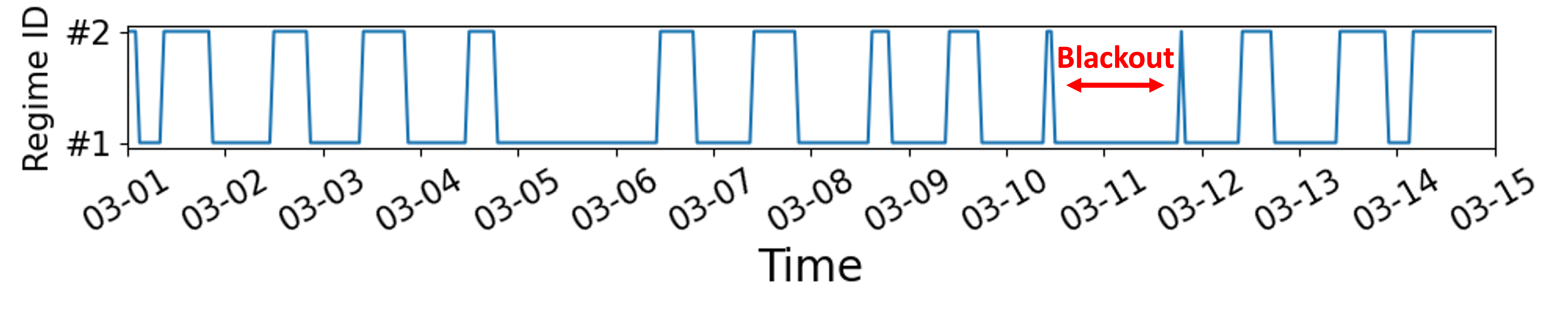
Motes. This dataset consists of temperature measurements from the $54$ sensors deployed in the Intel Berkeley Research Lab ⁴⁴4https://db.csail.mit.edu/labdata/labdata.html. We use hourly data for the first two weeks (03-01 $\sim$ 03-14). Originally, $9.6\%$ of the data is missing, including a blackout from 03-10 to 03-11 where all the values are missing.

5.1.2. Data preprocessing

We generate a synthetic missing block at a length of $0\sim 5\%$ of the data length and place it randomly until the total missing rate reaches $\{10,20,\dots 80\%\}$ . Thus, a missing block can be longer than $0.05T$ when it overlaps. An additional $10\%$ of missing values are added for hyperparameter tuning. Each dataset feature is normalized independently using a z-score so that each dataset has a zero mean and a unit variance.

5.1.3. Comparison methods

We compare our method with state-of-the-art imputation methods ranging from classical baselines (Linear and Quadratic), MF-based methods (SoftImpute, CDRec and TRMF), SSM-based methods (DynaMMo and DCMF), to DL-based methods (BRITS, SAITS and TIDER).

•

Linear/Quadratic ⁵⁵5https://pandas.pydata.org/docs/reference/api/pandas.DataFrame.interpolate.html use linear/quadratic equations to interpolate missing values.
•

SoftImpute (Mazumder et al., 2010) first fills in missing values with zero, then alternates between recovering the missing values and updating the SVD using the recovered matrix.
•

CDRec (Khayati et al., 2014) is a memory-efficient algorithm that iterates centroid decomposition (CD) and missing value imputation until they converge.
•

TRMF (Yu et al., 2016) is based on MF that imposes temporal dependency among the data points with the AR model.
•

DynaMMo (Li et al., 2009) first fills in missing values using linear interpolation and then uses the EM algorithm to iteratively recover missing values and update the LDS model.
•

DCMF (Cai et al., 2015a) adds a contextual constraint to SSM and captures inter-correlation by a predefined network. As suggested in the original paper, we give the cosine similarity between each pair of time series calculated after linear interpolation as a predefined network. This method is similar to MissNet if we set $K=1$ , employ a predefined network that is fixed throughout the algorithm, and eliminate the effect of regime-switching and network inference models from MissNet.
•

BRITS (Cao et al., 2018) imputes missing values according to hidden states from bidirectional RNN.
•

SAITS (Du et al., 2023) is a self-attention-based model that jointly optimizes imputation and reconstruction to perform the missing value imputation of multivariate time series.
•

TIDER (LIU et al., 2022) learns disentangled seasonal and trend representations by employing a neural network combined with MF.

5.1.4. Hyperparameter setting

For MissNet, we use the latent dimensions of $10,30$ and $15$ for Synthetic, MotionCapture and Motes, respectively, and we set $\lambda=1.0,\alpha=0.5$ for all datasets. We set the correct number of regimes on Synthetic datasets; we vary $K=\{1,2,3\}$ for other datasets. We list the detailed hyperparameter settings for the baselines in Appendix B.2.

5.1.5. Evaluation metric

To evaluate the effectiveness, we use Root Mean Square Error (RMSE) of the observed time series (Cai et al., 2015a).

5.2. Results

5.2.1. Q1. Effectiveness

We show the effectiveness of MissNet over baselines in missing value imputation.

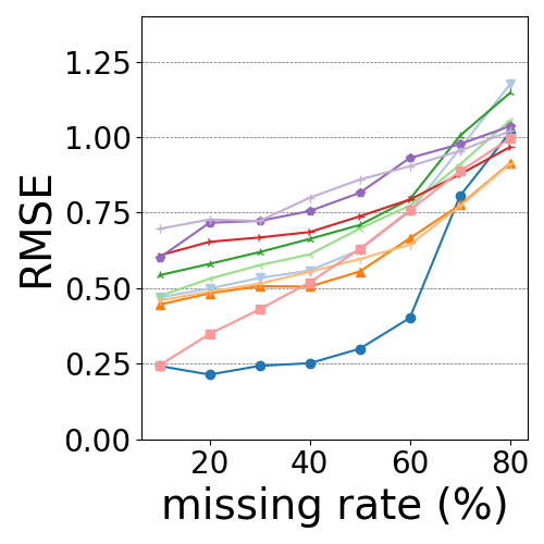
Synthetic. Fig. 3 (a) and (b) show the results obtained with Synthetic datasets. SSM and MF-based methods perform worse with PatternB than with PatternA due to the increased complexity of data. DL-based methods, especially BRITS, are less affected thanks to their high modeling power. MissNet significantly outperforms DCMF for PatternB although it produces similar results for PatternA. This is because DCMF fails to capture inter-correlation with PatternB since it can only use one predefined network and cannot afford a change of network. Meanwhile, MissNet can capture the inter-correlation for two different regimes thanks to our regime-switching model. However, MissNet fails to discover the correct transition when the missing rate exceeds $70\%$ , and RMSE becomes similar to DCMF.

MotionCapture and Motes. The results for MotionCapture and Motes datasets are shown in Fig. 3 (c) $\sim$ (l). We can see that MissNet and DCMF constantly outperform other baselines thanks to their ability to exploit inter-correlation explicitly.

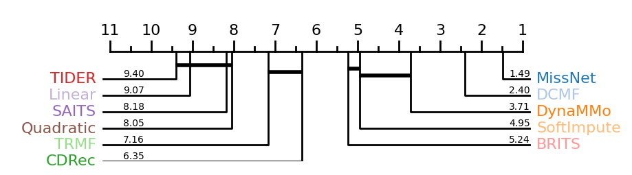
Fig. 4 shows the corresponding critical difference diagram for all missing rates based on the Wilcoxon-Holm method (Ismail Fawaz et al., 2019), where methods that are not connected by a bold line are significantly different in average rank. This confirms that MissNet significantly outperforms other methods, including DCMF, in average rank. Our algorithm for repeatedly inferring networks and the use of $\ell_{1}$ -norm enables the inference of adequate networks for imputation, contributing to better results than DCMF, which uses cosine similarity as a predefined network that may contain spurious correlations in the presence of missing values. Note that MissNet and DCMF exhibit only minor differences when the missing rate is low ( $10\%$ ) because a plausible predefined network can be calculated from observed data.

Classical Linear and Quadratic baselines are unsuitable for imputing missing blocks since they impute missing values mostly from neighboring observed points and cannot capture temporal patterns when there are large gaps. DL-based methods lack sufficient training data and are not suitable for the data we use here, making them perform particularly poorly at a high missing rate, as also noted in (Khayati et al., 2020). MF-based methods, SoftImpute and CDRec, have a higher RMSE than SSM-based methods since they do not model the temporal dynamics of the data. TRMF utilizes temporal dependency with the AR model, however, it can only capture certain lags specified on the hyperparameter of the AR model. SSM-based methods are superior in imputation to other groups owing to their ability to capture temporal dependency in latent space. DynaMMo implicitly captures inter-correlation in latent space. Therefore, it is no match for MissNet or DCMF.

Fig. 5 demonstrates the results for the MotionCapture Run dataset (missing rate $=60\%$ ). We compare the imputation result for the sensor at RKNE provided by the top five methods in terms of average rank, including MissNet, in Fig. 5 (a). BRITS and SoftImpute fail to capture the dynamics of time series while providing a good fit to observed values. The imputation of DynaMMo is smooth, but some parts are imprecise since it cannot explicitly exploit inter-correlation. MissNet and DCMF can effectively exploit other observed features associated with RKNE, thereby accurately imputing missing values where other methods fail (e.g., $T=20\sim 40,60\sim 80$ ). Fig. 5 (b) shows the sensor network of Y-coordinate values obtained by MissNet plotted on the human body, where a green/yellow dot (node) indicates a sensor placed on the front/back of the body and the thickness and color (blue/red) of the edges are the value and sign (positive/negative) of partial correlations, respectively. We can see that the sensors located close together have edges, meaning they are conditionally dependent given all other sensor values. For example, the sensor at RKNE has edges between RTHI, RSHN, LKNE, and LTHI. They are located to RKNE nearby and show similar dynamics, thus it is reasonable to consider that they are connected. Since MissNet can infer such a meaningful network from partially observed data, the imputation of MissNet is more accurate than that of DCMF.

5.2.2. Hyperparameter sensitivity

We take the Motes dataset and show the impact of hyperparameters: the latent dimension $L$ , the network parameter $\alpha$ , and the sparse parameter $\lambda$ . We show the mean RMSE of all missing rates.

Latent dimension. Fig. 6 (a) shows the impact of $L$ . As $L$ becomes larger, the model’s fitting against the observed data increases. As we can see, the RMSE is constantly decreasing as $L$ increases and stabilizes after $15$ . This shows that MissNet does not overfit the observed data even for a large $L$ .

Network parameter. $\alpha$ determines the contributions of inter-correlation and temporal dependency to learning $\dot{\bm{U}}$ . If $\alpha=0$ , the contextual matrix $\dot{\bm{S}}$ is ignored. If $\alpha=1$ , only $\dot{\bm{S}}$ is considered for learning $\dot{\bm{U}}$ . Fig. 6 (b) shows the results of varying $\alpha$ and they are robust except when $\alpha=1$ (RMSE $=0.76$ ). We can see that $\alpha=0.4$ shows the best result, indicating that both temporal dependency and inter-correlation are important for precise imputation.

Sparse parameter. $\lambda$ controls the sparsity of the networks $\dot{\bm{\Theta}}$ through $\ell_{1}$ -norm. The bigger $\lambda$ becomes, the more sparse the networks become, resulting in MissNet considering only strong interplay. By contrast, when $\lambda$ is small, MissNet considers insignificant interplays. Fig. 6 (c) shows the impact of $\lambda$ . We can see that the sparsity of the networks affects the accuracy, and the best $\lambda$ exists between $0.1$ and $10$ . Thus, the $\ell_{1}$ -norm constraint helps MissNet to exploit important relationships.

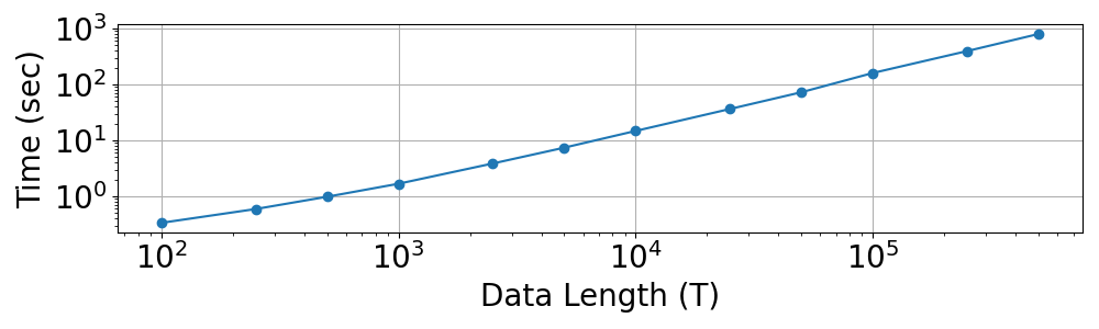
5.2.3. Q2. Scalability

We test the scalability of the MissNet algorithm by changing the number of the data length ( $T$ ) in PatternA. Fig. 7 shows the computation time for one iteration plotted with the data length. As it shows, our proposed MissNet algorithm scales linearly with regard to the data length $T$ .

5.2.4. Q3. Interpretability

We demonstrate how MissNet helps us understand data. We have shown an example with the MotionCapture Run dataset in Fig. 5 (b) where MissNet provides an interpretable network. Here, we demonstrate the results on the Motes dataset (missing rate $=30\%$ ) of MissNet ( $K=2$ ). Fig. 8 (a) shows the regime assignments $\bm{F}$ , and MissNet mostly assigns night hours to regime $\#1$ and working hours (about $9$ am. to $10$ pm.) to regime $\#2$ , suggesting that they have different networks. Fig. 8 (b) and (c) show the networks for regimes $\#1$ and $\#2$ obtained by MissNet plotted on the building layout. The sensor numbers in the figure are plotted on the actual sensor deployments. As we can see, the two regimes have different networks, and a common feature is that the neighboring sensors tend to form edges, which aligns with our expectations, considering that the sensors measure temperature and, thus, neighboring sensors correlate. The network of regime $\#2$ has more edges than that of $\#1$ , and the edges are $1.2$ times longer on average, which might be caused by air convection due to the movement of people during working hours. Consequently, MissNet provides regime assignments and sparse networks, which help us understand how data can be separated and important relationships for imputation.

6. Conclusion

In this paper, we proposed an effective missing value imputation method for multivariate time series, namely MissNet, which captures temporal dependency based on latent space and inter-correlation by the inferred networks while discovering regimes. Our proposed method has the following properties: (a) Effective: it outperforms the state-of-the-art algorithms for multivariate time series imputation. (b) Scalable: the computation time of MissNet scales linearly with regard to the length of the data. (c) Interpretable: it provides sparse networks and regime assignments, which help us understand the important relationships for imputation visually. Our extensive experiments demonstrated the above properties of MissNet.

Acknowledgements.

The authors would like to thank the anonymous referees for their valuable comments and helpful suggestions. This work was supported by JSPS KAKENHI Grant-in-Aid for Scientific Research Number JP21H03446, JP22K17896, NICT JPJ012368C03501, JST-AIP JPMJCR21U4, JST CREST JPMJCR23M3.

References

(1)
Alcaraz and Strodthoff (2022) Juan Miguel Lopez Alcaraz and Nils Strodthoff. 2022. Diffusion-based time series imputation and forecasting with structured state space models. arXiv preprint arXiv:2208.09399 (2022).
Bansal et al. (2021) Parikshit Bansal, Prathamesh Deshpande, and Sunita Sarawagi. 2021. Missing Value Imputation on Multidimensional Time Series. Proc. VLDB Endow. 14, 11 (jul 2021), 2533–2545.
Berrevoets et al. (2023) Jeroen Berrevoets, Fergus Imrie, Trent Kyono, James Jordon, and Mihaela van der Schaar. 2023. To impute or not to impute? missing data in treatment effect estimation. In International Conference on Artificial Intelligence and Statistics. PMLR, 3568–3590.
Boyd et al. (2011) Stephen P. Boyd, Neal Parikh, Eric Chu, Borja Peleato, and Jonathan Eckstein. 2011. Distributed Optimization and Statistical Learning via the Alternating Direction Method of Multipliers. Found. Trends Mach. Learn. 3, 1 (2011), 1–122.
Cai et al. (2015a) Yongjie Cai, Hanghang Tong, Wei Fan, and Ping Ji. 2015a. Fast mining of a network of coevolving time series. In Proceedings of the 2015 SIAM International Conference on Data Mining. SIAM, 298–306.
Cai et al. (2015b) Yongjie Cai, Hanghang Tong, Wei Fan, Ping Ji, and Qing He. 2015b. Facets: Fast comprehensive mining of coevolving high-order time series. In KDD. 79–88.
Cao et al. (2018) Wei Cao, Dong Wang, Jian Li, Hao Zhou, Lei Li, and Yitan Li. 2018. Brits: Bidirectional recurrent imputation for time series. Advances in neural information processing systems 31 (2018).
Chambon et al. (2018) Stanislas Chambon, Mathieu N Galtier, Pierrick J Arnal, Gilles Wainrib, and Alexandre Gramfort. 2018. A deep learning architecture for temporal sleep stage classification using multivariate and multimodal time series. IEEE Transactions on Neural Systems and Rehabilitation Engineering 26, 4 (2018), 758–769.
Chen and Sun (2021) Xinyu Chen and Lijun Sun. 2021. Bayesian temporal factorization for multidimensional time series prediction. IEEE Transactions on Pattern Analysis and Machine Intelligence 44, 9 (2021), 4659–4673.
Cini et al. (2021) Andrea Cini, Ivan Marisca, and Cesare Alippi. 2021. Filling the g_ap_s: Multivariate time series imputation by graph neural networks. arXiv preprint arXiv:2108.00298 (2021).
Dabrowski et al. (2018) Joel Janek Dabrowski, Ashfaqur Rahman, Andrew George, Stuart Arnold, and John McCulloch. 2018. State Space Models for Forecasting Water Quality Variables: An Application in Aquaculture Prawn Farming (KDD ’18). Association for Computing Machinery, New York, NY, USA, 177–185.
Du et al. (2023) Wenjie Du, David Côté, and Yan Liu. 2023. Saits: Self-attention-based imputation for time series. Expert Systems with Applications 219 (2023), 119619.
Fan et al. (2023) Yangxin Fan, Xuanji Yu, Raymond Wieser, David Meakin, Avishai Shaton, Jean-Nicolas Jaubert, Robert Flottemesch, Michael Howell, Jennifer Braid, Laura Bruckman, Roger French, and Yinghui Wu. 2023. Spatio-Temporal Denoising Graph Autoencoders with Data Augmentation for Photovoltaic Data Imputation. Proc. ACM Manag. Data 1, 1, Article 50 (may 2023), 19 pages. https://doi.org/10.1145/3588730
Fox et al. (2008) Emily Fox, Erik Sudderth, Michael Jordan, and Alan Willsky. 2008. Nonparametric Bayesian learning of switching linear dynamical systems. Advances in neural information processing systems 21 (2008).
Friedman et al. (2008) Jerome Friedman, Trevor Hastie, and Robert Tibshirani. 2008. Sparse inverse covariance estimation with the graphical lasso. Biostatistics 9, 3 (2008), 432–441.
Ghahramani (1998) Zoubin Ghahramani. 1998. Learning dynamic Bayesian networks. Springer Berlin Heidelberg, Berlin, Heidelberg, 168–197.
Hairi et al. (2019) N Hairi, Hanghang Tong, and Lei Ying. 2019. NetDyna: mining networked coevolving time series with missing values. In 2019 IEEE International Conference on Big Data (Big Data). IEEE, 503–512.
Hallac et al. (2017a) David Hallac, Youngsuk Park, Stephen P. Boyd, and Jure Leskovec. 2017a. Network Inference via the Time-Varying Graphical Lasso. In KDD. 205–213.
Hallac et al. (2017b) David Hallac, Sagar Vare, Stephen P. Boyd, and Jure Leskovec. 2017b. Toeplitz Inverse Covariance-Based Clustering of Multivariate Time Series Data. In KDD. 215–223.
Ismail Fawaz et al. (2019) Hassan Ismail Fawaz, Germain Forestier, Jonathan Weber, Lhassane Idoumghar, and Pierre-Alain Muller. 2019. Deep learning for time series classification: a review. Data mining and knowledge discovery 33, 4 (2019), 917–963.
Jing et al. (2021) Baoyu Jing, Hanghang Tong, and Yada Zhu. 2021. Network of tensor time series. In Proceedings of the Web Conference 2021. 2425–2437.
Khayati et al. (2014) Mourad Khayati, Michael Böhlen, and Johann Gamper. 2014. Memory-efficient centroid decomposition for long time series. In 2014 IEEE 30th International Conference on Data Engineering. IEEE, 100–111.
Khayati et al. (2020) Mourad Khayati, Alberto Lerner, Zakhar Tymchenko, and Philippe Cudré-Mauroux. 2020. Mind the gap: an experimental evaluation of imputation of missing values techniques in time series. In Proceedings of the VLDB Endowment, Vol. 13. 768–782.
Kolar and Xing (2012) Mladen Kolar and Eric P Xing. 2012. Estimating sparse precision matrices from data with missing values. In International Conference on Machine Learning. 635–642.
Li et al. (2009) Lei Li, James McCann, Nancy S Pollard, and Christos Faloutsos. 2009. Dynammo: Mining and summarization of coevolving sequences with missing values. In KDD. 507–516.
LIU et al. (2022) SHUAI LIU, Xiucheng Li, Gao Cong, Yile Chen, and YUE JIANG. 2022. Multivariate Time-series Imputation with Disentangled Temporal Representations. In The Eleventh International Conference on Learning Representations.
Liu et al. (2020) Yuehua Liu, Tharam Dillon, Wenjin Yu, Wenny Rahayu, and Fahed Mostafa. 2020. Missing value imputation for industrial IoT sensor data with large gaps. IEEE Internet of Things Journal 7, 8 (2020), 6855–6867.
Ma et al. (2008) Hao Ma, Haixuan Yang, Michael R Lyu, and Irwin King. 2008. Sorec: social recommendation using probabilistic matrix factorization. In Proceedings of the 17th ACM conference on Information and knowledge management. 931–940.
Malte Londschien and Bühlmann (2021) Solt Kovács Malte Londschien and Peter Bühlmann. 2021. Change-Point Detection for Graphical Models in the Presence of Missing Values. Journal of Computational and Graphical Statistics 30, 3 (2021), 768–779.
Mazumder et al. (2010) Rahul Mazumder, Trevor Hastie, and Robert Tibshirani. 2010. Spectral regularization algorithms for learning large incomplete matrices. The Journal of Machine Learning Research 11 (2010), 2287–2322.
Mohan et al. (2014) Karthik Mohan, Palma London, Maryam Fazel, Daniela Witten, and Su-In Lee. 2014. Node-Based Learning of Multiple Gaussian Graphical Models. J. Mach. Learn. Res. 15, 1 (jan 2014), 445–488.
Monti et al. (2014) Ricardo Pio Monti, Peter Hellyer, David Sharp, Robert Leech, Christoforos Anagnostopoulos, and Giovanni Montana. 2014. Estimating time-varying brain connectivity networks from functional MRI time series. NeuroImage 103 (2014), 427–443.
Namaki et al. (2011) A. Namaki, A.H. Shirazi, R. Raei, and G.R. Jafari. 2011. Network analysis of a financial market based on genuine correlation and threshold method. Physica A: Statistical Mechanics and its Applications 390, 21 (2011), 3835–3841.
Obata et al. (2024) Kohei Obata, Koki Kawabata, Yasuko Matsubara, and Yasushi Sakurai. 2024. Dynamic Multi-Network Mining of Tensor Time Series. In Proceedings of the ACM on Web Conference 2024 (WWW ’24). 4117–4127.
Papadimitriou et al. (2005) Spiros Papadimitriou, Jimeng Sun, and Christos Faloutsos. 2005. Streaming pattern discovery in multiple time-series. (2005).
Pavlovic et al. (1999) Vladimir Pavlovic, James M Rehg, Tat-Jen Cham, and Kevin P Murphy. 1999. A dynamic Bayesian network approach to figure tracking using learned dynamic models. In Proceedings of the seventh IEEE international conference on computer vision, Vol. 1. IEEE, 94–101.
Qin et al. (2020) Zhen Qin, Yibo Zhang, Shuyu Meng, Zhiguang Qin, and Kim-Kwang Raymond Choo. 2020. Imaging and fusing time series for wearable sensor-based human activity recognition. Information Fusion 53 (2020), 80–87.
Ren et al. (2023) Xiaobin Ren, Kaiqi Zhao, Patricia Riddle, Katerina Taškova, Lianyan Li, and Qingyi Pan. 2023. DAMR: Dynamic Adjacency Matrix Representation Learning for Multivariate Time Series Imputation. SIGMOD (2023). https://doi.org/10.1145/3589333
Rogers et al. (2013) Mark Rogers, Lei Li, and Stuart J Russell. 2013. Multilinear dynamical systems for tensor time series. Advances in Neural Information Processing Systems 26 (2013).
Shadbahr et al. (2023) Tolou Shadbahr, Michael Roberts, Jan Stanczuk, Julian Gilbey, Philip Teare, Sören Dittmer, Matthew Thorpe, Ramon Viñas Torné, Evis Sala, Pietro Lió, Mishal Patel, Jacobus Preller, Ian Selby, Anna Breger, Jonathan R. Weir-McCall, Effrossyni Gkrania-Klotsas, Anna Korhonen, Emily Jefferson, Georg Langs, Guang Yang, Helmut Prosch, Judith Babar, Lorena Escudero Sánchez, Marcel Wassin, Markus Holzer, Nicholas Walton, Pietro Lió, James H. F. Rudd, Tuomas Mirtti, Antti Sakari Rannikko, John A. D. Aston, Jing Tang, and Carola-Bibiane Schönlieb. 2023. The impact of imputation quality on machine learning classifiers for datasets with missing values. Communications Medicine 3, 1 (2023).
Shukla and Marlin (2021) Satya Narayan Shukla and Benjamin M Marlin. 2021. Multi-time attention networks for irregularly sampled time series. arXiv preprint arXiv:2101.10318 (2021).
Städler and Bühlmann (2012a) Nicolas Städler and Peter Bühlmann. 2012a. Missing values: sparse inverse covariance estimation and an extension to sparse regression. Statistics and Computing 22 (2012), 219–235.
Städler and Bühlmann (2012b) Nicolas Städler and Peter Bühlmann. 2012b. Missing values: sparse inverse covariance estimation and an extension to sparse regression. Statistics and Computing 22 (2012), 219–235.
Tashiro et al. (2021) Yusuke Tashiro, Jiaming Song, Yang Song, and Stefano Ermon. 2021. Csdi: Conditional score-based diffusion models for probabilistic time series imputation. Advances in Neural Information Processing Systems 34 (2021), 24804–24816.
Tomasi et al. (2021) Federico Tomasi, Veronica Tozzo, and Annalisa Barla. 2021. Temporal Pattern Detection in Time-Varying Graphical Models. In ICPR. 4481–4488.
Tomasi et al. (2018) Federico Tomasi, Veronica Tozzo, Saverio Salzo, and Alessandro Verri. 2018. Latent Variable Time-varying Network Inference. In KDD. 2338–2346. https://doi.org/10.1145/3219819.3220121
Tozzo et al. (2021) Veronica Tozzo, Federico Ciech, Davide Garbarino, and Alessandro Verri. 2021. Statistical Models Coupling Allows for Complex Local Multivariate Time Series Analysis. In KDD. 1593–1603.
Tozzo et al. (2020) Veronica Tozzo, Davide Garbarino, and Annalisa Barla. 2020. Missing Values in Multiple Joint Inference of Gaussian Graphical Models. In Proceedings of the 10th International Conference on Probabilistic Graphical Models (Proceedings of Machine Learning Research, Vol. 138), Manfred Jaeger and Thomas Dyhre Nielsen (Eds.). PMLR, 497–508.
Viterbi (1967) Andrew Viterbi. 1967. Error bounds for convolutional codes and an asymptotically optimum decoding algorithm. IEEE transactions on Information Theory 13, 2 (1967), 260–269.
Wang et al. (2023a) Dingsu Wang, Yuchen Yan, Ruizhong Qiu, Yada Zhu, Kaiyu Guan, Andrew Margenot, and Hanghang Tong. 2023a. Networked time series imputation via position-aware graph enhanced variational autoencoders. In KDD. 2256–2268.
Wang et al. (2023b) Xu Wang, Hongbo Zhang, Pengkun Wang, Yudong Zhang, Binwu Wang, Zhengyang Zhou, and Yang Wang. 2023b. An Observed Value Consistent Diffusion Model for Imputing Missing Values in Multivariate Time Series. In KDD. 2409–2418.
Yi et al. (2016) Xiuwen Yi, Yu Zheng, Junbo Zhang, and Tianrui Li. 2016. ST-MVL: filling missing values in geo-sensory time series data. In Proceedings of the 25th International Joint Conference on Artificial Intelligence.
Yoon et al. (2018a) Jinsung Yoon, James Jordon, and Mihaela Schaar. 2018a. Gain: Missing data imputation using generative adversarial nets. In International conference on machine learning. PMLR, 5689–5698.
Yoon et al. (2018b) Jinsung Yoon, William R Zame, and Mihaela van der Schaar. 2018b. Estimating missing data in temporal data streams using multi-directional recurrent neural networks. IEEE Transactions on Biomedical Engineering 66, 5 (2018), 1477–1490.
Yu et al. (2016) Hsiang-Fu Yu, Nikhil Rao, and Inderjit S. Dhillon. 2016. Temporal Regularized Matrix Factoriztion for High-dimensional Time Series Prediction. In Advances in Neural Information Processing Systems 28.
Zhang and Balzano (2016) Dejiao Zhang and Laura Balzano. 2016. Global convergence of a grassmannian gradient descent algorithm for subspace estimation. In Artificial Intelligence and Statistics. PMLR, 1460–1468.

Appendix A Proposed model

A.1. Symbols

Table 2 lists the main symbols we use throughout this paper.

A.2. Complexity analysis

Proof of Lemma 1.

Proof.

The overall time complexity is composed of four parts by taking the most time-consuming part of equations for each iteration considering $N>N_{t},L$ : the complexity for the inference of $\bm{Z}$ and $\bm{F}$ is $O(K^{2}\sum_{t=1}^{T}(L^{3}+L^{2}N_{t}+LN_{t}^{2}+N_{t}^{3}))$ related to Eq. (13) and Eq. (15); the inference of $\dot{\bm{V}}$ is $O(KL^{2}N^{2})$ (Eq. (19)); M step is $O(KTL^{2}N)$ related to the calculation of $\dot{\bm{U}}$ (Eq. (21)); and the update of $\dot{\bm{\Theta}}$ is $O(KN^{3})$ (Eq. (23)). Thus, the overall time complexity is $O(\#iter\cdot(K^{2}\sum_{t=1}^{T}(L^{3}+L^{2}N_{t}+LN_{t}^{2}+N_{t}^{3})+KL^{2}N^{2}+KTL^{2}N+KN^{3}))$ . ∎

Proof of Lemma 2.

Proof.

The space complexity is composed of three parts: storing input dataset $\bm{X}$ is $O(TN)$ ; intermediate values in E step are $O(K^{2}TL^{2}+KL^{2}N)$ ; and storing parameter set is $O(KN^{2})$ . Thus, the overall space complexity is $O(TN+K^{2}TL^{2}+KL^{2}N+KN^{2})$ . ∎

Table 2. Symbols and definitions.

Symbol	Definition
$\bm{X}$	Multivariate time series $\bm{X}=\{\bm{x}_{1},\bm{x}_{2},\dots,\bm{x}_{T}\}\in\mathbb{R}^{N\times T}$
$\bm{W}$	Indicator matrix $\bm{W}\in\mathbb{R}^{N\times T}$
$\tilde{\bm{X}}$	Partially observed multivariate time series $\tilde{\bm{X}}=\bm{W}\circ\bm{X}$
$\hat{\bm{X}}$	Inputed multivariate time series
$\bm{Z}$	Time series latent states $\bm{Z}\in\mathbb{R}^{L\times T}$
$\bm{V}^{(k)}$	Contextual latent factor of $k^{th}$ -regime $\bm{V}^{(k)}\in\mathbb{R}^{L\times N}$
$\bm{S}^{(k)}$	Contextual matrix of $k^{th}$ -regime $\bm{S}^{(k)}\in\mathbb{R}^{N\times N}$
$\bm{B}$	Transition matrix $\bm{B}\in\mathbb{R}^{L\times L}$
$\bm{U}^{(k)}$	Observation matrix of $k^{th}$ -regime $\bm{U}^{(k)}\in\mathbb{R}^{N\times L}$
$\bm{F}$	Regime assignments $\bm{F}\in\mathbb{R}^{K\times T}$
$\bm{\rho}^{(k)}$	Mean vector of $k^{th}$ -regime $\bm{\rho}^{(k)}\in\mathbb{R}^{N}$
$\bm{\Theta}^{(k)}$	Inverse covariance matrix (i.e., network) of $k^{th}$ -regime $\bm{\Theta}^{(k)}\in\mathbb{R}^{N\times N}$
$N$	Number of features
$T$	Number of timesteps
$L$	Number of latent dimensions
$K$	Number of regimes
$\alpha$	Trade-off between temporal dependency and inter-correlation
$\lambda$	Parameter for $\ell_{1}$ -norm that regulates network sparsity

A.3. Updating parameters

The parameters are updated as follows:

	$\displaystyle\bm{B}^{new}$	$\displaystyle=\bigg{(}\sum_{t=2}^{T}\mathbb{E}[\bm{z}_{t}\bm{z}^{\prime}_{t-1}]\bigg{)}\bigg{(}\sum_{t=2}^{T}\mathbb{E}[\bm{z}_{t-1}\bm{z}^{\prime}_{t-1}]\bigg{)}^{-1},$
	$\displaystyle\bm{z}_{0}^{new}$	$\displaystyle=\mathbb{E}[\bm{z}_{1}],$
	$\displaystyle\bm{\Psi}_{0}^{new}$	$\displaystyle=\mathbb{E}[\bm{z}_{1}\bm{z}^{\prime}_{1}]-\mathbb{E}[\bm{z}_{1}]\mathbb{E}[\bm{z}^{\prime}_{1}],$

	$\displaystyle(\sigma_{\bm{Z}}^{2})^{new}=$	$\displaystyle\frac{1}{(T-1)L}\textrm{tr}\bigg{(}\sum_{t=2}^{T}\mathbb{E}[\bm{z}_{t}\bm{z}^{\prime}_{t}]-\bm{B}\sum_{t=2}^{T}\mathbb{E}[\bm{z}_{t}\bm{z}^{\prime}_{t}]\bigg{)},$
	$\displaystyle(\sigma_{\bm{X}^{(k)}}^{2})^{new}=$	$\displaystyle\frac{1}{\sum_{t=1(\bm{f}_{t}=k)}^{T}\sum_{i=1}^{N}\bm{W}_{i,t}}$
		$\displaystyle\bigg{[}\sum_{t=1(\bm{f}_{t}=k)}^{T}tr\bigg{(}(\bar{\bm{U}}^{(k)}_{t})^{new}\mathbb{E}[\bm{z}_{t}\bm{z}^{\prime}_{t}](\bar{\bm{U}}^{(k)}_{t})^{new^{\prime}}\bigg{)}$
		$\displaystyle+\sum_{t=1(\bm{f}_{t}=k)}^{T}\bigg{(}(\bar{\bm{x}}_{t})^{\prime}\bar{\bm{x}}_{t}-2(\bar{\bm{x}}_{t})^{\prime}((\bar{\bm{U}}^{(k)}_{t})^{new}\mathbb{E}[\bm{z}_{t}])\bigg{)}\bigg{]},$
	$\displaystyle(\sigma_{\bm{S}^{(k)}}^{2})^{new}=$	$\displaystyle\frac{1}{N^{2}}\bigg{[}\sum_{j=1}^{N}\bigg{(}\bm{s}^{(k)^{\prime}}_{j}\bm{s}^{(k)}_{j}-2\bm{s}^{(k)^{\prime}}_{j}((\bm{U}^{(k)})^{new}\mathbb{E}[\bm{v}^{(k)}_{j}])\bigg{)}$
		$\displaystyle+tr\bigg{(}(\bm{U}^{(k)})^{new}(\sum_{j=1}^{N}\mathbb{E}[\bm{v}^{(k)}_{j}\bm{v}^{(k)^{\prime}}_{j}])(\bm{U}^{(k)new})^{\prime}\bigg{)}\bigg{]},$
(26)		$\displaystyle(\sigma_{\bm{V}^{(k)}}^{2})^{new}=$	$\displaystyle\frac{1}{NL}\sum_{j=1}^{N}\textrm{tr}(\mathbb{E}[\bm{v}^{(k)}_{j}\bm{v}^{(k)^{\prime}}_{j}]).$

Appendix B Experiments

B.1. Synthetic data generation

We first generate a latent factor containing a linear trend, a sinusoidal seasonal pattern, and a noise, $\bm{Z}_{i,t}=\sin(2\pi\frac{\beta}{T}t)+\gamma t+\eta$ , s.t. $1<\beta<20,0.3<|\gamma|<1,\eta\sim\mathcal{N}(0,0.3)$ , where $\bm{Z}\in\mathbb{R}^{L\times T}$ . We then project the latent factor with object matrix $\bm{X}=\bm{U}^{(k)}\bm{Z}$ , where $\bm{X}\in\mathbb{R}^{N\times T}$ , and $\bm{U}^{(k)}\in\mathbb{R}^{N\times L}$ is a random graph created as follows (Mohan et al., 2014):

(1)

Set $\bm{U}^{(k)}$ equal to the adjacency matrix of an Erdős-Rényi directed random graph, where every edge has a $20\%$ chance of being selected.
(2)

Set selected edge $\bm{U}^{(k)}_{i,j}\sim$ Uniform $([-0.6,-0.3]\cup[0.3,0.6])$ , where $\bm{U}^{(k)}_{i,j}$ denotes the weight between variables $i$ and $j$ .

We set $T=1000,N=50,L=10$ . We generate two types of synthetic data, PatternA and PatternB, five times each, where $K=1,2$ , respectively. In PatternB, the regime switches every $200$ timesteps.

B.2. Hyperparameters

We describe the hyperparameters of the baselines. For Synthetic datasets, we give a latent dimension of $10$ for all baselines. For a fair comparison, we set the latent dimension of the SSM-based methods at the same value as MissNet. For the MF-based methods, we vary the latent dimension $\{3,5,10,15,20,30,40\}$ . We vary the AR parameter for TRMF $\{[1,2,3,4,5],[1,24]\}$ . To learn the DL-based methods, we add $10\%$ of the data as missing values for training the model. We vary the window size $\{16,32,T\}$ . Other hyperparameters are the same as the original codes.

Appendix C Discussion

While MissNet achieved superior performance against state-of-the-art baselines in missing value imputation, here, we mention two limitations of MissNet in terms of sparse network inference and data size.

As mentioned in Section 5.2.1, MissNet fails to discover the correct transition when the missing rate exceeds $70\%$ . However, we claim that MissNet failing to discover the correct transition when the missing rate exceeds $70\%$ is reasonable; rather, correctly discovering transition up to $60\%$ is valuable. Several studies (Tozzo et al., 2020; Kolar and Xing, 2012; Städler and Bühlmann, 2012b) tackled the sparse network inference under the existence of missing values. They aim to infer the correct network and, thus, only utilize the observed value for the network inference. Since observing a complete pair at a high missing rate is rare, it is difficult to infer the correct network. Therefore, the maximum missing rate in their experiments is $30\%$ . Although the experimental settings are different from ours, we can say that the task of sparse network inference in the presence of missing values itself is challenging.

As shown in the experiments, MissNet performs well even when a relatively small number of samples ( $T$ ) and a large number of features ( $N$ ) since MissNet is a parametric model and we assume the sparse networks to capture inter-correlation. This cannot be achieved by DL models, which contain a massive number of parameters that require a large amount of $T$ , especially when $N$ is large since all the relationships between features need to be learned. However, unlike DL models, the increased number of samples may not greatly improve MissNet’s performance as it has a much smaller number of parameters than DL models, even though switching sparse networks increases the model’s flexibility.

	$\displaystyle\bm{\mu}_{t\|t-1,k,l}$	$\displaystyle=\bm{B}\bm{\mu}_{t-1\|t-1,k,l},$
	$\displaystyle\bm{\mu}_{t\|t,k,l}$	$\displaystyle=\bm{\mu}_{t\|t-1,k,l}+\bm{D}_{t,k,l}(\bar{\bm{x}}_{t}-\bar{\bm{U}}^{(k)}_{t}\bm{B}\bm{\mu}_{t\|t-1,k,l}),$
	$\displaystyle\bm{\Psi}_{t\|t-1,k,l}$	$\displaystyle=\bm{B}\bm{\Psi}_{t-1\|t-1,k,l}\bm{B}^{\prime}+\sigma_{\bm{Z}}^{2}\bm{I},$
	$\displaystyle\bm{\Psi}_{t\|t,k,l}$	$\displaystyle=(\bm{I}-\bm{D}_{t,k,l}\bar{\bm{U}}^{(k)}_{t})\bm{\Psi}_{t-1\|t-1,k,l},$
(13)		$\displaystyle\bm{D}_{t,k,l}$	$\displaystyle=\bm{\Psi}_{t\|t-1,k,l}\bar{\bm{U}}^{(k)^{\prime}}_{t}(\bar{\bm{U}}^{(k)}_{t}\bm{\Psi}_{t\|t-1,k,l}\bar{\bm{U}}^{(k)^{\prime}}_{t}+\sigma_{\bm{X}^{(k)}}^{2}\bm{I})^{-1},$

Mining of Switching Sparse Networks for Missing Value Imputation in Multivariate Time Series

Abstract.

1. Introduction

2. Related work

3. Preliminaries

3.1. Problem definition

Problem 1 (Multivariate Time Series Missing Value Imputation).

3.2. Graphical lasso

4. Proposed MissNet

4.1. Optimization model

4.2. Algorithm

4.2.1. E-step

4.2.2. M-step

4.2.3. Update 𝑺˙\dot{\bm{S}}

4.2.4. Overall algorithm

4.3. Complexity analysis

Lemma 0.

Proof.

Lemma 0.

Proof.

5. Experiments

5.1. Experimental setup

5.1.1. Datasets

5.1.2. Data preprocessing

5.1.3. Comparison methods

5.1.4. Hyperparameter setting

5.1.5. Evaluation metric

5.2. Results

5.2.1. Q1. Effectiveness

5.2.2. Hyperparameter sensitivity

5.2.3. Q2. Scalability

5.2.4. Q3. Interpretability

6. Conclusion

Acknowledgements.

References

Appendix A Proposed model

A.1. Symbols

A.2. Complexity analysis

Proof.

Proof.

A.3. Updating parameters

Appendix B Experiments

B.1. Synthetic data generation

B.2. Hyperparameters

Appendix C Discussion

4.2.3. Update $\dot{\bm{S}}$