Minimum-Cost State-Flipped Control
for Reachability of Boolean Control Networks
using Reinforcement Learning
Abstract
This paper proposes model-free reinforcement learning methods for minimum-cost state-flipped control in Boolean control networks (BCNs). We tackle two questions: 1) finding the flipping kernel, namely the flip set with the smallest cardinality ensuring reachability, and 2) deriving optimal policies to minimize the number of flipping actions for reachability based on the obtained flipping kernel. For question 1), Q-learning's capability in determining reachability is demonstrated. To expedite convergence, we incorporate two improvements: i) demonstrating that previously reachable states remain reachable after adding elements to the flip set, followed by employing transfer learning, and ii) initiating each episode with special initial states whose reachability to the target state set are currently unknown. Question 2) requires optimal control with terminal constraints, while Q-learning only handles unconstrained problems. To bridge the gap, we propose a BCN-characteristics-based reward scheme and prove its optimality. Questions 1) and 2) with large-scale BCNs are addressed by employing small memory Q-learning, which reduces memory usage by only recording visited action-values. An upper bound on memory usage is provided to assess the algorithm's feasibility. To expedite convergence for question 2) in large-scale BCNs, we introduce adaptive variable rewards based on the known maximum steps needed to reach the target state set without cycles. Finally, the effectiveness of the proposed methods is validated on both small- and large-scale BCNs.
Index Terms:
Boolean control networks, model-free, reachability, reinforcement learning, state-flipped control.I Introduction
Gene regulatory networks are a crucial focus in systems biology. The concept of Boolean networks was first introduced in 1969 by Kauffman [1] as the earliest model for gene regulatory networks. Boolean networks consist of several Boolean variables, each of which takes a value of ``0” or ``1” to signify whether the gene is transcribed or not. As gene regulatory networks often involve external inputs, Boolean networks were further developed into Boolean control networks (BCNs), which incorporate control inputs to better describe network behaviors.
State-flipped control is an innovative method used to change the state of specific nodes in BCNs, flipping them from ``1" to ``0" or from ``0" to ``1". In the context of systems biology, state-flipped control can be achieved through gene regulation techniques such as transcription activator-like effector repression and clustered regularly interspaced short palindromic repeats activation [2]. State-flipped control is a powerful control method that minimally disrupts the system structure. From a control effectiveness standpoint, state-flipped control enables BCNs to achieve any desired state with an in-degree greater than 0 [3, 4]. In contrast, state feedback control can only steer BCNs towards the original reachable state set, which is a subset of states with an in-degree greater than 0. Another highly effective control method is pinning control, but it has the drawback of causing damage to the network structure, unlike state-flipped control. State-flipped control was first proposed by Rafimanzelat to study the controllability of attractors in BNs [5]. Subsequently, to achieve stabilization, authors in [6] and [7] respectively considered flipping a subset of nodes after the BN had passed its transient period and flipping a subset of nodes in BCNs at the initial step. Zhang et al. further extended the concept of state-flipped control from BCNs to switched BCNs [8]. Considering that previous research has primarily focused on one-time flipping [5, 6, 8, 7], which may hinder the achievement of certain control objectives, a more comprehensive form of state-flipped control that permits multiple flipping actions was introduced to study stabilization in BNs and BCNs [3, 4]. Furthermore, to minimize control costs, the concept of flipping kernel was proposed [4, 3], representing the smallest set of nodes that can accomplish the control objectives. In this paper, we extend the existing studies by investigating problems including finding flipping kernels, under joint control proposed by [3]. These joint controls involve the combination of state-flipped controls and control inputs as defined in [3].
Closely tied to stabilization and controllability, reachability is a prominent area that requires extensive exploration. It involves determining whether a system can transition from an initial subset of states to a desired subset of states. This concept holds significant importance in domains such as genetic reprogramming and targeted drug development, where the ability to transform networks from unfavorable states to desirable ones is pivotal [6]. Previous studies [9, 10, 11, 12] have proposed various necessary and sufficient conditions for reachability in BCNs and their extensions. Additionally, an algorithm has been developed to identify an optimal control policy that achieves reachability in the shortest possible time [10]. In the context of BCNs under state-flipped control, the analysis of reachability between two states can be conducted using the semi-tensor product [3].
Despite extensive studies on the reachability of BCNs, there are still unresolved issues in this field. These problems can be categorized into three aspects.
-
.
Firstly, the existing literature [9, 10, 11, 12] focuses on determining whether reachability can be achieved under certain control policies, without optimizing control costs. This is significant in both practical applications and theoretical research. For instance, in the development of targeted drugs, an increasing number of target points raises the difficulty level. Additionally, it is desirable to minimize the frequency of drug usage by patients to achieve expense savings and reduce drug side effects. If we formulate this problem as an optimal control problem, our objective is to find the flipping kernel and minimize the number of flipping actions. Emphasizing the identification of flipping kernels is more critical than minimizing flipping actions, as it significantly reduces the dimensionality of joint control, thereby exponentially alleviating the computational complexity when minimizing flipping actions. It is worth mentioning that achieving reachability while optimizing control costs poses an optimization problem with terminal constraint. To the best of our knowledge, conventional optimal control techniques such as the path integral approach and policy iteration [13, 14, 15, 16], which rely on predetermined cost functions, are deemed unsuitable for our study. This is primarily due to the challenge of expressing the objective of simultaneously minimizing control costs and achieving terminal goals, namely, ``achieving reachability," solely through a cost function.
-
.
Secondly, the model-free scenario requires special consideration, especially considering the increasing complexity associated with accurately modeling systems with numerous BCN nodes. While model-free approaches exist in the PBCNs field [17, 18, 4, 3, 19, 20], they address different challenges compared to ours. Additionally, there are ongoing investigations into cost reduction problems [9, 10, 11, 12, 21, 22, 23]. However, these studies are conducted under the assumption of known or partially known models.
-
.
Thirdly, the existing methods in the fields of BCN reachability[9, 10, 11, 12, 21] are limited in their applicability to small-scale BCNs. Several interesting approaches have been proposed for handling large BCNs, emphasizing controllability and stability [24, 25, 26]. However, these references concentrate on optimization goals slightly different from ours. They aim to minimize the set of controlled nodes, namely, the dimension of the controller. In contrast, our objective is not only to reduce the controller dimension but also to further minimize flipping actions, namely, the frequency of control implementation.
Considering the aforementioned issues, we aim to design minimum-cost state-flipped control for achieving reachability in BCNs, in the absence of a known system model. Specifically, we address the following questions:
-
0)
How to find the flipping kernel for reachability?
-
0)
Building on question 1), how can we determine the control policies that minimize the number of required flipping actions to achieve reachability?
Questions 1) and 2) are the same as 1) and 2) mentioned in the abstract. They are reiterated here for clarity purposes.
To tackle these questions, we turn to reinforcement learning-based methods. Compared with the semi-tensor product approach, reinforcement learning-based methods are suitable for model-free scenarios, which aligns with our considered setting. Moreover, reinforcement learning eliminates the need for matrix calculations and offers the potential to handle large-scale BCNs. In particular, we consider the extensively applied -learning (L) method, which has been successful in solving control problems in BCNs and their extensions [17, 18, 4, 3, 19]. For reachability problems of large-scale BCNs, an enhanced L method has been proposed by [20], providing a reliable foundation for this study. When compared to the deep -learning method [27], which is also suitable for large-scale BCNs, the method proposed in [20] is favored due to its theoretical guarantees of convergence [28].
Taken together, we propose an improved L to address questions 1)- 3). Our work's main contributions are as follows:
-
0.
Regarding question 1), unlike the semi-tensor product method proposed in [4, 3], our approach is model-free. We demonstrate that reachability can be determined using L and propose improved L with faster convergence compared to the traditional one [29]. Firstly, transfer learning (TL) [30] is integrated under the premise that the transferred knowledge is proven to be effective. Then, special initial states are incorporated into L, allowing each episode to begin with an unknown reachability state, thereby eliminating unnecessary computations.
-
0.
Question 2) involves optimal control with terminal constraints, while L only handles unconstrained problems. To bridge this gap, a BCN-characteristics-based reward scheme is proposed. Compared to other model-free approaches [17, 18, 4, 3, 19, 20], we first tackle a complex problem while providing rigorous theoretical guarantees.
-
0.
Compared to matrix-based methods [4, 3] and deep reinforcement techniques [17, 19, 18], our algorithms are suitable for large-scale BCNs with convergence guarantee. In contrast to [20], the memory usage in the presented problem is clarified to be not directly related to the scale of the BCNs, and an upper bound is provided to evaluate algorithm suitability. Further, To accelerate convergence in question 2), a modified reward scheme is introduced.
The paper progresses as follows: Section II provides an overview of the system model and defines the problem statement. Section III introduces the reinforcement learning method. In Section IV, fast iterative L and small memory iterative L for large-scale BCNs are presented to identify the flipping kernel for reachability. In Section V, to minimize the number of flipping actions, L with a BCN-characteristics-based reward setting and that with dynamic rewards for large-scale BCNs are proposed. Algorithm complexity is detailed in Section VI. Section VII validates the proposed method. Finally, conclusions are drawn in Section VIII.
We use the following notations throughout this paper:
-
•
, , , denote the sets of non-negative integers, non-negative real numbers, real numbers, and real number matrices, respectively.
-
•
denotes the expected value operator and var denotes the variance. denotes the probability of event occurring given that event has occurred.
-
•
For a set , denotes the cardinal number of .
-
•
For , denotes the maximal value of the elements in .
-
•
The relative complement of set in set is denoted as .
-
•
There are four basic operations on Boolean variables, which are ``not", ``and", ``or", and ``exclusive or", expressed as , , , and , respectively.
-
•
, and .
II Problem Formulation
This section introduces the system model, with a specific focus on BCNs under state-flipped control. Subsequently, we outline the problems under investigation.
II-A System Model
II-A1 BCNs
A BCN with nodes and control inputs is defined as
| (1) | ||||
where is a logical function, represents the node at time step , and represents the control input at time step . All nodes at time step are grouped together in the vector . Similarly, all control inputs at time step are represented by .
II-A2 State-flipped Control
Considering that not all nodes in a BCN can be flipped, we refer to the set of all flippable nodes as a flip set . At each time step , a flipping action is selected. According to the flipping action , the flip function is defined as
| (2) | ||||
Note that to achieve a specific control objective, it is not necessary to flip all the nodes in the set . The flipping kernel, denoted as , is defined as the flip set with the minimum cardinality required to achieve reachability.
II-A3 BCNs under State-flipped Control
Based on the definition of BCNs and state-flipped control, a BCN with nodes and a flip set is defined as
| (3) |
II-B Problems of Interests
II-B1 Problem 1. Flipping Kernel for Reachability
To better illustrate Problem 1, we first define reachability.
[31]. For system (3), let be the initial subset, and be the target subset. is said to be reachable from if and only if, for any initial state , there exists a sequence of joint control pairs , such that reaches a target state .
Based on Definition 1, we define the specific problem to be considered. In some cases, it is not necessary to flip all nodes in the set for system (3) to achieve reachability. To reduce the control cost, we hope the nodes that need to be flipped as few as possible. The above problem can be transformed into finding the flipping kernel for reachability, which satisfies
| (4) | ||||
| s.t. | ||||
It is worth noting that flipping kernel may not be unique, as there can be multiple ways to achieve reachability with the minimum cardinality through flipping.
II-B2 Problem 2. Minimum Flipping Actions for Reachability
Based on the flipping kernel obtained from Problem 1 (4), we aim to determine the optimal policy, under which the reachability can be achieved with minimum flipping actions. This problem can be formulated as finding the policy that satisfies
| (5) | ||||
where denotes the number of nodes to be flipped at time step , and represents the terminal time step when a terminal state emerges. The terminal and initial states are represented by and , respectively. Note that the optimal policy may not be unique, as multiple policies can achieve reachability with minimal flipping actions.
III Preliminaries
In this section, we introduce a reinforcement learning method, specifically focusing on the Markov decision process and the -learning algorithm.
III-A Markov Decision Process
Markov decision process provides the framework for reinforcement learning, which is represented as a quintuple . and denote the state space and action space, respectively. The discount factor weighs the importance of future rewards. The state-transition probability represents the chance of transitioning from state to under action . denotes the expected reward obtained by taking action at state that transitions to . At each time step , an agent interacts with the environment to determine an optimal policy. Specificly, the agent observes and selects , according to the policy . Then, the environment returns and . The agent evaluates the reward received for taking action at state and then updates its policy . Define as the return. The goal of the agent is to learn the optimal policy , which satisfies
| (6) |
where is the the expected value operator following policy , and is the set of all admissible policies. The state-value and the action-value are and , respectively. The Bellman equations reveal the recursion of and , which are given as follows:
| (7) | ||||
The optimal state-value and action-value are defined as
| (8) | ||||
For problems under the framework of Markov decision process, the optimal policy can be obtained through L. In the following, we introduce L.
III-B -Learning
L is a classical algorithm in reinforcement learning. The purpose of L is to enable the agent to find an optimal policy through its interactions with the environment. , namely, the estimate of , is recorded and updated every time step as follows:
| (9) |
where is the learning rate, and .
In terms of action selection, -greedy method is used
| (10) |
where is the probability of selecting the corresponding action, , and is an action randomly selected from .
[28]. converges to the fixed point with probability one under the following conditions:
-
0.
and .
-
0.
is finite.
-
0.
and are finite.
-
0.
If , all policies lead to a cost-free terminal state.
Once L converges, the optimal policy is obtained:
| (11) |
IV Flipping Kernel for Reachability
To solve Problem 1 (4), we propose three algorithms: iterative L, fast iterative L, and small memory iterative L. Fast iterative L enhances convergence efficiency over iterative L. Meanwhile, small memory iterative L is designed specifically for large-scale BCNs (3).
IV-A Markov Decision Process for Finding Flipping Kernel
The premise for using L is to structure the problem within the framework of Markov decision process. We represent Markov decision process by the quintuple , where and are the state space and action space, respectively. The state and the action are defined as and , respectively. The reward is given as follows:
| (12) |
To incentivize the agent to reach as quickly as possible, we set the discount factor .
Assuming the agent is aware of the dimensions of and but lacks knowledge of and , meaning the agent does not comprehend the system dynamics (3). Through interactions with the environment, the agent implicitly learns about , , refines estimation of , and enhances its understanding of .
IV-B Iterative Q-Learning for Finding Flipping Kernel
Under the reward setting (12), it is worthwhile to investigate methods for determining the reachability of BCNs defined by equation (3). To answer this question, we present Theorem 1.
. For system (3), assume that and equation (9) is utilized for updating . System (3) from any state in is reachable to state set if and only if, there exists a such that .
. (Necessity) Assume that system (3) from any state in is reachable to state set . Without loss of generality, suppose that there is only one and one . Then, there exists a joint control pair sequence , such that will reach the target state . We apply to , then we obtain a trajectory , where . Meanwhile, means that will transform into when is taken.
As L iterates, all state-action-state pairs are constantly visited [28]. Therefore, there can be a case where the state-action-state pairs , , , …, are visited one after another, and in between, other state-action-state pairs can also exist. This case causes the values in the -table to transition from all zeros to some being positive. Furthermore, we assume that this case initially occurs at time step . Then, the corresponding change of action-value from zero to positive is given by , where since . Additionally, due to the absence of negative rewards and the fact that initial action-values are all 0, it follows that for all . Thus, after the update, we have . According to (9), at , it follows that . Similarly, for any , it follows that .
Next, we prove that there exists such that , where , based on mathematical induction. The proof is divided into two parts. Firstly, there exists such that where , according to the proof in the previous paragraph. Second, we prove that if is visited at time step and , then . Since is visited at time step , it follows that . In the updated formula, we have , and . Furthermore, since , it implies that . Consequently, we have . According to mathematical induction, there exists such that . Since holds, we have .
(Sufficiency) Suppose that there exists such that . Without loss of generality, we assume that there is only one as well as one , , and . Then, according to the updated formula , where is the subsequent state of , at least one of the following two cases exists:
-
•
Case 1. There exist and such that .
-
•
Case 2. satisfies .
In Case 1, we have . It implies that system (3) from state is reachable to state set in one step.
In terms of Case 2, let us consider the condition under which , meaning that there exists an action such that . We define the action-value, which changes from 0 to a positive number, as . Here, denotes the time step of the change of the action-value, and corresponds to the state-action pair. Since the initial -values are all 0, it follows that if and only if . This implies that system (3) from state is reachable to state set within one step, leading to . Next, for any , occurs if and only if , or , where is a state that has satisfied for based on the previously defined conditions. This means that for , at least one of the following two events has taken place: either is reachable from ; or a state , which can reach , is reachable from . In both cases, it implies that is reachable from . Thus, if , it follows that is reachable from . This, in turn, implies that is also reachable from . Based on the analysis of Cases 1 and 2, if holds for all , then is reachable from .
. The key for L to judge the reachability for system (3) lies in exploration (10) and update rule (9).
. For system (3), is reachable from if and only if there exists such that is -step reachable from .
. Without loss of generality, let us assume that there is a trajectory from to whose length is greater than . Then, there must be at least one that is visited repeatedly. If we remove the cycle from to , the trajectory length will be less than .
Based on Theorem 1 and Lemma 2, we present Algorithm 1 for finding flipping kernels. First, we provide the notation definitions used in Algorithm 1. denotes the combinatorial number of flip sets with the given nodes in . represents the flip set with the given nodes. denotes the number of episodes, where ``Episode" is a term from reinforcement learning, referring to a period of interaction that has passed through time steps from any initial state . is the maximum time step, which should exceed the length of the trajectory from to . One can refer to Lemma 2 for the setting of .
The core idea of Algorithm 1 is to incrementally increase the flip set size from to in step 18 when reachability isn't achieved with flip sets of size . Specifically, step 4 fixes the flip set , followed by steps 5-16 assessing reachability under that flip set, guided by Theorem 1. Upon identifying the first flipping kernel (when the condition in step 12 is met), the cardinality of the kernel is determined. This leads to setting as per step 13, along with step 2 to prevent ineffective access to a larger flip set. After evaluating system reachability under all flip sets with nodes, steps 20-24 present the algorithm's results.
Although Algorithm 1 is efficient, there is room for improvement. The next section outlines techniques to enhance its convergence efficiency.
IV-C Fast Iterative Q-learning for Finding Flipping Kernel
In this subsection, we propose Algorithm 2, known as fast iterative L for finding the flipping kernels, which improves the convergence efficiency. The main difference between Algorithm 2 and Algorithm 1 can be classified into two aspects. 1) Special initial states: Algorithm 2 selects initial states strategically instead of randomly. 2) TL: Algorithm 2 utilizes the knowledge gained from achieving reachability with smaller flip sets to search for flipping kernels for larger flip sets.
IV-C1 Special Initial States
The main concept behind selecting special initial states is to avoid visiting once we determine that is reachable from it. Instead, we focus on states in that have not been identified as reachable. With this approach in mind, we modify step 7 in Algorithm 1 into
| (13) |
The validity of Theorem 1 remains when special initial states are added to iterative L, as the trajectory from the states in that are reachable to can still be visited.
IV-C2 Transfer-learning
Let and represent the -table with flip sets and respectively, where . The relationship between and is explained in Theorem 2 below.
. For any state-action pairs , if with flip set , then holds for flip set .
. It is evident that the action space for flip set is the subset of the action space for flip set , namely, . Therefore, if system (3) from state is reachable to state with flip set , namely, there exists a trajectory , the reachability still holds with flip set . This is because the trajectory exists for . Thus, if is reachable from with flip set , then the reachability holds with flip set . According to Theorem 1, for all , if with flip set , then holds for flip set .
Motivated by the above results, we consider TL [30]. TL enhances the learning process in a new task by transferring knowledge from a related task that has already been learned. In this context, we employ TL by initializing the -table for flip set with the knowledge gained from the -tables for flip sets , namely
| (14) |
where represents the -table associated with flip set . Based on this idea, we refine step 5 and include steps 7 and 9 in Algorithm 2 compared to Algorithm 1.
Algorithm 2 improves the convergence efficiency compared to Algorithm 1. However, Algorithm 2 is not suitable for large-scale BCNs. Specifically, the operation of iterative L is based on a -table that has values. The number of values in the table grows exponentially with and , and can be expressed as . When and are large, iterative L becomes impractical because the -table is too large to store on a computer. Therefore, we propose an algorithm in the following subsection, which can be applied to large-scale BCNs.
IV-D Small Memory Iterative Q-Learning for Finding Flipping Kernel of Large-scale BCNs
In this subsection, we present Algorithm 3, named small memory iterative L, which is inspired by the work of [20]. This algorithm serves as a solution for identifying flipping kernels in large-scale BCNs. The core idea behind Algorithm 3 is to store action-values only for visited states, instead of all , to reduce memory consumption. To implement this idea, we make adjustments to step 5 in Algorithm 1 and introduce additional steps 10-12 in Algorithm 3. Subsequently, we offer detailed insights into the effectiveness of Algorithm 3 and its applicability.
Since Algorithm 3 only stores action-values for visited states, it reduces the number of required action-values. Specifically, let's define is reachable from , . Then, we can observe that is the total number of visitable states, where represents the union of sets. Therefore, we can conclude that the number of required action-values using Algorithm 3 is , which is a number not exceeding . Next, we present Theorem 3 to provide an estimation of . To better understand the theorem, we first introduce Definition 2.
[4]. The in-degree of is defined as the number of states which can reach in one step with where .
. Define the in-degree of is greater than 0, . Then, it follows that .
. The state transition process can be divided into two steps. For any , according to , it is firstly flipped into . Second, based on , namely, , tranfers to . According to the second step of the state transition process and the definition of , we have . Due to the arbitrariness of , it follows that is reachable from in one step, . Since contains all states, the condition `in one step' can be removed. Define is reachable from , . So, we have . Notice that the only difference between the sets and is the domain of the initial states. Since we have , it follows that . Therefore, it can be concluded that .
Algorithm 3 can reduce the number of entries stored in the -table from to , where . However, we acknowledge that when the size of becomes excessively large, L faces certain limitations. It is important to note that Algorithm 3 offers a potential solution for addressing problems in large-scale BCNs, as opposed to the conventional L approach, which is often deemed inapplicable. In fact, the value of is not directly related to . Specifically, large-scale BCNs with low connectivity will result in a small number of . Traditional L preconceives to store values in the -table, which not only restricts the ability to handle problems in large-scale systems but also lacks practicality. In contrast, Algorithm 3 allows agents to explore and determine the significant information that needs to be recorded. This approach provides an opportunity to solve the reachability problems of large-scale BCNs.
. The idea of utilizing special initial states and TL in Algorithm 2 can also be incorporated into Algorithm 3. The hybrid algorithm proposed has two major advantages: improved convergence efficiency and expanded applicability to large-scale BCNs.
V Minimum Flipping Actions for Reachability
In this section, we aim to solve Problem 2 (5). First, we propose a reward setting in which the highest return is achieved only when the policy successfully reaches the goal. Then, we propose two algorithms for obtaining the optimal policies: L for small-scale BCNs, and small memory L for large-scale ones.
V-A Markov Decision Process for Minimizing Flipping Actions
Since L will be used to find , we first construct the problem into the framework of Markov decision process. Let Markov decision process be the quintuple . To guide the agent in achieving the goal with minimal flipping actions, we define as follows:
| (15) |
where represents the weight. The reward consists of two parts. The first component is ``-1'', which is assigned when the agent has not yet reached . This negative feedback encourages the agent to reach the goal as soon as possible. The second component is ``'', which incentivizes the agent to use as few flipping actions as possible to reach the goal. Since we aim to minimize the cumulative flipping actions at each time step, we set indicating that future rewards are not discounted in importance.
. The following analysis is based on the assumption that system (3) from any state in is reachable to state set . The validity of this assumption can be verified using Theorem 1.
The selection of plays a crucial role in effectively conveying the goal (5) to the agent. If is too small, the objective of achieving reachability as soon as possible will submerge the objective of minimizing flipping actions. To illustrate this issue more clearly, let us consider an example.
. Without loss of generality, we assume that there is only one and one . Suppose that there exist two policies and . When we start with and take , we obtain the trajectory without any flipping action. If we take , the trajectory with 2 flipping actions will be obtained. It can be calculated that , since the agent takes 4 steps to achieve reachability without flipping actions. Meanwhile, , since the agent takes 1 step to achieve reachability with 2 flipping actions. If we set , then it will follow that . Therefore, the obtained optimal policy requires more flipping actions to achieve reachability, which does not contribute to finding for equation (5).
Furthermore, although a high value of the parameter ``" assists in reducing flipping actions for reachability, it can present challenges in reinforcement learning. Convergence in these algorithms relies on a finite reward variance, as specified in the second condition of Lemma 1. As ``" approaches infinity, this criterion cannot be satisfied. Additionally, an excessively large value of ``" may increase reward variance, resulting in greater variability in estimated state values and subsequently affecting the speed of algorithm convergence [32]. Hence, establishing a lower bound for ``" becomes crucial to facilitate algorithm convergence while ensuring goal attainment.
So, what should be the appropriate value of to achieve the goal (5)? To address this question, sufficient conditions that ensure the optimality of the policy are proposed in Theorem 4 and Corollary 1. The main concept is to select a value of such that and , where satisfies the goal (5).
. For system (3), if , where is the maximum number of steps required from any initial states to reach without cycles, then the optimal policy obtained based on (15) satisfies the goal (5).
. Without loss of generality, it is assumed that there is only one . We classify all and prove that, under the condition that , the policy with the highest state-value satisfies the goal (5). For all , we can divide them into two cases:
For Case 1, . The value of is insufficient for to be optimal. For Case 2, we divide it into two sub-cases:
Next, we compare the magnitude of and . Let us assume that it takes steps with flipping actions, and steps with flipping actions for system (3) from state to reach state set under and , respectively. Then, we can obtain and . It is calculated that
| (16) |
Since more flipping actions are taken under than to achieve reachability, then one has .
Regarding the relationship between and , there are two categories:
-
•
Category 1. .
-
•
Category 2. .
For Category 1, it's obvious that . For Category 2, we divide into two cases.
Next, we prove . For Case 2.1.1, we have the following inequalities
| (17) |
where is the minumum length of the trajectory from to . Substitute (17) into (16), we have . Since , it follows that .
In the following, we discuss Case 2.1.2. Note that implies that at least one is visited repeatedly, according to Lemma 2. If we eliminate the cycle from the trajectory, then its length will be no greater than , and its flipping actions are fewer. This indicates that there exists such that and . Thus, is consistent with Case 2.1.1. Based on the proof in the previous paragraph, we have . Also, it is easy to see that . Therefore, it can be concluded that has the highest return compared with and .
After analyzing various cases, we deduce that when holds, one of the following two conditions must be satisfied: 1) ; 2) There exists an alternative policy that achieves reachability with fewer flipping actions compared to , satisfying the conditions and . Namely, yielding the highest satisfies the goal (5).
In Theorem 4, the knowledge of is necessary. If is unknown, we can deduce the following corollary according to Lemma 2: .
. Two points should be clarified for Theorem 4 and Corollary 1. First, following Theorem 4 or Corollary 1, we do not obtain all that satisfy the goal (5), but rather the that satisfies the goal (5) with the shortest time to achieve reachability. Second, Theorem 4 and Corollary 1 provide sufficient conditions but not necessary conditions for the optimality of the obtained policy, in that (17) uses the inequality scaling technique.
V-B Q-Learning for Finding Minimum Flipping Actions
In this subsection, we propose Algorithm 4 for finding minimum flipping actions for the reachability of BCNs under state-flipped control.
Next, we discuss the requirements for the parameters. In terms of , it should be larger than the maximum length of the trajectory from to without any cycle. Otherwise, the agent may not be able to reach the terminal state in before the episode ends, which violates condition 4) of Lemma 1. Furthermore, it should satisfy , ensuring the exploration of the agent. Hence, the policies during learning are non-deterministic, namely, all the policies can lead to a state , which satisfies condition 4) of Lemma 1.
Algorithm 4 is capable of finding for small-scale BCNs under state-flipped control. However, it becomes inapplicable when the values of and are too large since the -table is too large to be stored in computer memory. This motivates us to utilize small memory L in Section IV-D.
V-C Fast Small Memory Q-Learning for Finding Minimum Flipping Actions of Large-scale BCNs
In this section, we propose Algorithm 5 called the fast small memory L for finding the minimum flipping actions required to achieve reachability in large-scale BCNs under state-flipped control. Algorithm 5 differs from Algorithm 4 in two aspects.
Firstly, Algorithm 5 only records the action values of the visited states, as reflected in steps 1 and 9-11. This approach is similar to that employed in Algorithm 3. Secondly, in Algorithm 5, the parameter which affects changes from a constant to a variable that is dynamically adjusted according to is in the -table, as shown in steps 4-6. As the agent explores more states, increases and finally equals to . Here, we do not simply set based on Corollary 1, in that for large-scale BCNs, the value of is so large causing the weight for using fewer flipping actions to outweigh the importance of achieving reachability as soon as possible. This can lead to confusion for the agent. Specifically, at the beginning of the learning process, the agent receives large negative feedback when taking flipping actions, but less negative feedback when it fails to achieve reachability. The agent will only realize that taking flipping actions is worthwhile for achieving reachability when the accumulation of the negative feedback ``-1" for not realizing reachability exceeds that of ``'' for flipping nodes. The larger the , the longer the process will take. To address this issue, we introduce the scaling for to accelerate the process. The key concept behind this scaling method is to leverage the knowledge acquired by the agent while ensuring that the conditions in Theorem 4 are met to guarantee the optimality of the policy. We provide further explanation of this approach in Theorem 5.
. For a BCN under state-flipped control (3), if it holds that , then the optimal policy obtained according to (15) satisfies the goal (5).
. First, we prove that is reachable from only if, there exists such that is -step reachable from . Assume that is reachable from . According to Definition 1, for any initial state , there exists a trajectory , where . According to the definition of , each state in the above trajectory is in . Similar to the proof of Lemma 2, for any initial state , there exists a trajectory from to whose length satisfies .
Next, we prove that after sufficient exploration by the agent. Since , and , we have . From the proof in the previous paragraph, we know that , therefore, we have . By applying Theorem 4, we can guarantee the optimality of the policy.
Thus, Algorithm 5 with the introduction of the variable still satisfies the goal defined by (5). Furthermore, it speeds up the learning process. Regarding the parameter settings of Algorithm 5, the initial can be set according to is in the -table, where the -table is the one obtained from Algorithm 3.
In summary, Algorithm 5 reduces the number of values to be stored from to by recording only the visited states. This approach is especially effective for solving large-scale BCN problems. Meanwhile, to accelerate the learning process, is set as a variable that will converge to a value that is larger than .
VI Computational Complexity
The time complexities of Algorithms 1-5 involve selecting the optimal value from a pool of up to action-values per step, resulting in O() complexity. For Algorithms 1, 2, and 3, the total number of steps is expressed as iter and iter respectively, revealing pre- and post-flipping kernel discovery iterations. Introducing early termination based on reachability conditions in Algorithms 1-3 reduces the number of episodes for the flip set with and , while Algorithm 2's efficiency ensures . Algorithms 4 and 5 require steps in total. Refer to Table I for a comprehensive overview of the time complexities of each algorithm.
Concerning space complexity, Algorithms 1 and 4 store all action-values in a -table, while Algorithm 2 additionally manages tables for subsets of the current flip set. In contrast, Algorithms 3 and 5 retain action-values for solely visited states. Details on the final space complexities for each algorithm can be found in Table I.
| Time complexity | Space complexity | |
|---|---|---|
| 1 | (iter1) | () |
| 2 | (iter2) | () |
| 3 | (iter1,3) | () |
| 4 | () | () |
| 5 | () | () |
VII Simulation
In this section, the performance of the proposed algorithms is shown. Two examples are given, which are a small-scale BCN with 3 nodes and a large-scale one with 27 nodes. For each example, the convergence efficiency of different algorithms to check the reachability, and with minimal flipping actions are shown.
VII-A A Small-scale BCN
. We consider a small-scale BCN with the combinational flip set , the dynamics of which is given as follows:
| (18) |
In terms of the reachability, we set and .
To find the flipping kernels of system (18), Algorithms 1 and 2 are utilized. As mentioned in section IV, Algorithm 2 has higher convergence efficiency compared with Algorithm 1. The result is verified in our simulation. To evaluate the convergence efficiency, the index named reachable rate is defined as follows:
| (19) |
where represents the number of that have been found to be reachable to at the end of the episode. For Algorithms 1 and 2, the flipping kernels utilized are and , respectively. The effectiveness of Algorithms 1 and 2 is shown in Fig. 1, where the reachable rates are the average rates obtained from 100 independent experiments. In terms of L with TL, the initial reachable rate is higher since the agent utilizes prior knowledge. For L with special initial states, the reachable rate increases faster than conventional L since the agent strategically selects the initial states. The best performance is achieved when both TL and special initial states are incorporated into L.
Next, Algorithm 4 is employed to determine the minimum number of flipping actions required for reachability. The optimal policy obtained is shown in Fig. 2.


Emphasizing that the system model in this paper is solely for illustrative purposes, we stress that the agent has no prior knowledge of the model.
The flipping kernels obtained through Algorithms 1 and 2 have been compared with those obtained using the model-based method proposed by [3]. Additionally, the policies depicted in Figs. 2 and 4 have been compared with other policies derived through enumeration. The results of these comparisons have verified that the flipping kernels and policies obtained are indeed optimal.
We utilize the method proposed by [3] solely to validate the optimality of the flipping kernel, without directly comparing its computational complexity or convergence speed. This is because the semi-tensor product method introduced by [3] requires prior knowledge of the system model, whereas our approach is model-free. Therefore, it would be unfair to make a direct comparison between the two methods.
VII-B A Large-scale BCN
. We consider a large-scale BCN with the combinational flip set , the dynamics of which is given as follows:
| (20) |
where . In terms of the reachability, we set and , where .

System (20) consists of 9 small-scale BCNs. In Fig. 3, it can be observed that the number of flipping actions and time steps required for system (20) to reach state set is relatively small. These two phenomena can be attributed to our intention of selecting an example that is easily verifiable for the optimal policy using the enumeration method. However, it should be noted that the proposed algorithms are applicable to all large-scale BCNs since the agent has no prior knowledge of the system model.
To obtain the flipping kernels of the large-scale system (20), Algorithm 3 is employed along with the integration of TL and special initial states. The convergence efficiency of the algorithms is demonstrated in Fig. 3. According to Fig. 3, the combination of small memory L with both TL and special initial states yields the best performance.
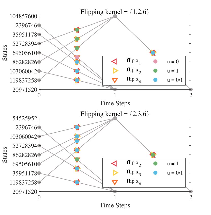
Subsequently, based on the flipping kernels and obtained from Algorithm 3, the optimal policy taking the minimal flipping actions to achieve the reachability is obtained using Algorithm 5. The resulting policy is displayed in Fig. 4. Notably, in terms of reward setting, if we set instead of utilizing a variable that changes according to is in the -table, the policy cannot converge to the optimal one even with 10 times episodes. This demonstrates the effectiveness of Algorithm 5. In Fig. 4, we simplify the state in decimal form, where a state at time step is defined as .
VII-C Details
The parameters are listed as follows.
-
•
In all algorithms, we set learning rate as , which satisfies condition 1) in Lemma 1.
-
•
The greedy rate in all algorithms is specified as , gradually reducing from 1 to 0.01 as increases.
-
•
We set for Algorithm 3 in Example 2 and with for Algorithm 5 in Example 3. These values of ensure the optimality of the obtained policy according to Corollary 1 and Theorem 4.
-
•
For Algorithms 1, 2, and 3, we set .
, , , and are selected based on the complexity of different examples and algorithms, as detailed in Table II.
| Example | Algorithm | ||||
| 2 | 1,2 | 100 | 10 | 1 | 0.6 |
| 3 | 3 | 1 | 0.6 | ||
| 2 | 4 | 100 | 0.01 | 0.85 | |
| 3 | 5 | 0.01 | 0.85 |
VIII Conclusion
This paper presents - reinforcement learning-based methods to obtain minimal state-flipped control for achieving reachability in BCNs, including large-scale ones. Two problems are addressed: 1) finding the flipping kernel, and 2) minimizing flipping actions based on the kernel.
For problem 1) with small-scale BCNs, fast iterative L is proposed. Reachability is determined using -values, while convergence is expedited through transfer learning and special initial states. Transfer learning migrates the -table based on the proven theorem that reachability preservation holds as the flip set size increases. Special initial states designate unknown reachability states to avoid redundant evaluation of known reachable states. For problem 1) with large-scale BCNs, we utilize small memory iterative L, which reduces memory usage by only recording visited action-values. Algorithm suitability is estimated via an upper bound on memory usage.
For problem 2) with small-scale BCNs, L with BCN-characteristics-based rewards is presented. The rewards are designed based on the maximum length of reachable trajectories without cycles (an upper bound is given). This allows the minimization of flipping actions under terminal reachability constraints to be simplified as an unconstrained optimal control problem. For problem 2) with large-scale BCNs, fast small memory L with variable rewards is proposed. In this approach, the rewards are dynamically adjusted based on the maximum length of explored reachable trajectories without cycles to enhance convergence efficiency, and their optimality is proven.
Considering the critical value of reachability in controllability, our upcoming research will investigate minimum-cost state-flipped control for controllability of BCNs using reinforcement methods. Specifically, we will address two key challenges: 1) identifying the flipping kernel for controllability of BCNs, and 2) minimizing the required flipping actions to achieve controllability. While our approach can effectively address challenges 1 and 2 for small-scale BCNs with minor adjustments, adapting it for large-scale BCNs with simple modifications is presently impractical. This will be the primary focus of our future research.
References
- [1] S. A. Kauffman, ``Metabolic stability and epigenesis in randomly constructed genetic nets,'' Journal of theoretical biology, vol. 22, no. 3, pp. 437–467, 1969.
- [2] M. Boettcher and M. McManus, ``Choosing the Right Tool for the Job: RNAi, TALEN, or CRISPR,'' Molecular Cell, vol. 58, no. 4, pp. 575–585, 2015.
- [3] Y. Liu, Z. Liu, and J. Lu, ``State-flipped control and Q-learning algorithm for the stabilization of Boolean control networks,'' Control Theory & Applications, vol. 38, pp. 1743–1753, 2021.
- [4] Z. Liu, J. Zhong, Y. Liu, and W. Gui, ``Weak stabilization of Boolean networks under state-flipped control,'' IEEE Transactions on Neural Networks and Learning Systems, vol. 34, pp. 2693–2700, 2021.
- [5] M. Rafimanzelat and F. Bahrami, ``Attractor controllability of Boolean networks by flipping a subset of their nodes,'' Chaos: An Interdisciplinary Journal of Nonlinear Science, vol. 28, p. 043120, 2018.
- [6] M. R. Rafimanzelat and F. Bahrami, ``Attractor stabilizability of Boolean networks with application to biomolecular regulatory networks,'' IEEE Transactions on Control of Network Systems, vol. 6, no. 1, pp. 72–81, 2018.
- [7] B. Chen, X. Yang, Y. Liu, and J. Qiu, ``Controllability and stabilization of Boolean control networks by the auxiliary function of flipping,'' International Journal of Robust and Nonlinear Control, vol. 30, no. 14, pp. 5529–5541, 2020.
- [8] Q. Zhang, J.-e. Feng, Y. Zhao, and J. Zhao, ``Stabilization and set stabilization of switched Boolean control networks via flipping mechanism,'' Nonlinear Analysis: Hybrid Systems, vol. 41, p. 101055, 2021.
- [9] R. Zhou, Y. Guo, Y. Wu, and W. Gui, ``Asymptotical feedback set stabilization of probabilistic Boolean control networks,'' IEEE Transactions on Neural Networks and Learning Systems, vol. 31, no. 11, pp. 4524–4537, 2019.
- [10] H. Li and Y. Wang, ``On reachability and controllability of switched Boolean control networks,'' Automatica, vol. 48, no. 11, pp. 2917–2922, 2012.
- [11] Y. Liu, H. Chen, J. Lu, and B. Wu, ``Controllability of probabilistic Boolean control networks based on transition probability matrices,'' Automatica, vol. 52, pp. 340–345, 2015.
- [12] J. Liang, H. Chen, and J. Lam, ``An improved criterion for controllability of Boolean control networks,'' IEEE Transactions on Automatic Control, vol. 62, no. 11, pp. 6012–6018, 2017.
- [13] L. Wang and Z.-G. Wu, ``Optimal asynchronous stabilization for Boolean control networks with lebesgue sampling,'' IEEE Transactions on Cybernetics, vol. 52, no. 5, pp. 2811–2820, 2022.
- [14] Y. Wu, X.-M. Sun, X. Zhao, and T. Shen, ``Optimal control of Boolean control networks with average cost: A policy iteration approach,'' Automatica, vol. 100, pp. 378–387, 2019.
- [15] S. Kharade, S. Sutavani, S. Wagh, A. Yerudkar, C. Del Vecchio, and N. Singh, ``Optimal control of probabilistic Boolean control networks: A scalable infinite horizon approach,'' International Journal of Robust and Nonlinear Control, vol. 33, no. 9, p. 4945–4966, 2023.
- [16] Q. Zhu, Y. Liu, J. Lu, and J. Cao, ``On the optimal control of Boolean control networks,'' SIAM Journal on Control and Optimization, vol. 56, no. 2, pp. 1321–1341, 2018.
- [17] A. Acernese, A. Yerudkar, L. Glielmo, and C. D. Vecchio, ``Reinforcement learning approach to feedback stabilization problem of probabilistic Boolean control networks,'' IEEE Control Systems Letters, vol. 5, no. 1, pp. 337–342, 2021.
- [18] P. Bajaria, A. Yerudkar, and C. D. Vecchio, ``Random forest Q-Learning for feedback stabilization of probabilistic Boolean control networks,'' in 2021 IEEE International Conference on Systems, Man, and Cybernetics (SMC), 2021, pp. 1539–1544.
- [19] Z. Zhou, Y. Liu, J. Lu, and L. Glielmo, ``Cluster synchronization of Boolean networks under state-flipped control with reinforcement learning,'' IEEE Transactions on Circuits and Systems II: Express Briefs, vol. 69, no. 12, pp. 5044–5048, 2022.
- [20] X. Peng, Y. Tang, F. Li, and Y. Liu, ``Q-learning based optimal false data injection attack on probabilistic Boolean control networks,'' 2023. [Online]. Available: https://api.semanticscholar.org/CorpusID:265498378
- [21] Z. Liu, Y. Liu, Q. Ruan, and W. Gui, ``Robust flipping stabilization of Boolean networks: A Q-learning approach,'' Systems & Control Letters, vol. 176, p. 105527, 2023.
- [22] J. Lu, R. Liu, J. Lou, and Y. Liu, ``Pinning stabilization of Boolean control networks via a minimum number of controllers,'' IEEE Transactions on Cybernetics, vol. 51, no. 1, pp. 373–381, 2021.
- [23] Y. Liu, L. Wang, J. Lu, and L. Yu, ``Pinning stabilization of stochastic networks with finite states via controlling minimal nodes,'' IEEE Transactions on Cybernetics, vol. 52, no. 4, pp. 2361–2369, 2022.
- [24] S. Zhu, J. Lu, D. W. Ho, and J. Cao, ``Minimal control nodes for strong structural observability of discrete-time iteration systems: Explicit formulas and polynomial-time algorithms,'' IEEE Transactions on Automatic Control, 2023. [Online]. doi: 10.1109/TAC.2023.3330263.
- [25] S. Zhu, J. Cao, L. Lin, J. Lam, and S.-i. Azuma, ``Towards stabilizable large-scale Boolean networks by controlling the minimal set of nodes,'' IEEE Transactions on Automatic Control, vol. 69, no. 1, pp. 174–188, 2024.
- [26] S. Zhu, J. Lu, S.-i. Azuma, and W. X. Zheng, ``Strong structural controllability of Boolean networks: Polynomial-time criteria, minimal node control, and distributed pinning strategies,'' IEEE Transactions on Automatic Control, vol. 68, no. 9, pp. 5461–5476, 2023.
- [27] H. V. Hasselt, A. Guez, and D. Silver, ``Deep reinforcement learning with double Q-learning,'' Proceedings of the AAAI Conference on Artificial Intelligence, vol. 30, no. 1, pp. 1–13, 2016.
- [28] T. Jaakkola, M. Jordan, and S. Singh, ``Convergence of stochastic iterative dynamic programming algorithms,'' Advances in neural information processing systems, vol. 6, p. 703–710, 1993.
- [29] C. J. Watkins and P. Dayan, ``Q-learning,'' Machine Learning, vol. 8, no. 3, pp. 279–292, 1992.
- [30] L. Torrey and J. Shavlik, ``Transfer learning,'' in Handbook of research on machine learning applications and trends: algorithms, methods, and techniques. IGI global, 2010, pp. 242–264.
- [31] R. Zhou, Y. Guo, and W. Gui, ``Set reachability and observability of probabilistic Boolean networks,'' Automatica, vol. 106, pp. 230–241, 2019.
- [32] E. Greensmith, P. L. Bartlett, and J. Baxter, ``Variance reduction techniques for gradient estimates in reinforcement learning,'' Journal of Machine Learning Research, vol. 5, no. 9, p. 1471–1530, 2004.