Minimizing Moments of AoI for Both Active and Passive Users through Second-Order Analysis

Recently, there has been a significant increase in the use of time-sensitive applications such as Internet of Things, vehicular networks, sensor networks, and drone systems for surveillance and reconnaissance. While traditional research has focused on optimizing the reliability and throughput of communication, these efforts often fall short in meeting the demands for fresh data. To address this, a performance metric known as age-of-information (AoI) was introduced [1] and has received increasing attention in recent literature [2, 3, 4, 5, 6, 7, 8, 9, 10, 11, 12, 13, 14, 15, 16, 17, 18, 19, 20, 21, 22, 23, 24, 25, 26, 27, 28, 29, 30, 31, 32].

Previous studies on AoI have commonly considered centralized control over transmission decisions [8, 9, 7, 10, 11, 12, 13] and queuing problems without transmission collisions [15, 18, 16, 19, 17]. However, centralized policies and collisions can lead to large overhead or extra communication, which can be a significant drawback in delay-sensitive applications such as the Internet of Things and transmission-sensitive applications like satellite communications.

To address this issue, we consider a random access network, where active users broadcast sensed data and multiple transmissions at the same time can cause collisions. Since there are no acknowledgements in broadcast, active users do not have any feedback information on collisions. This makes recent feedback-based algorithms for AoI optimization [22, 23, 24, 25, 21, 26] inapplicable.

Additionally, we consider that the network has silent observers, referred to as passive users, who share the same channel as active users. Passive users aim to observe out-of-network radio activities in the same channel but do not make any transmissions. Examples of passive users include sensors detecting malicious jammers, receivers of satellite communications, and radio telescopes tracking celestial objects. The coexistence of passive and active users can improve channel utilization, as passive users can obtain valuable observations when no active user is transmitting.

As AoI depends on previous successful transmissions, memoryless random access algorithms, such as slotted ALOHA, are not suitable for optimizing AoI. Therefore, we consider that each active user follows a Markov process to determine its transmission activities. Furthermore, instead of only considering the mean of AoI, we consider the moments of AoI, which can offer insights into the variance and the maximum value of AoI.

The goal of this paper is to minimize the weighted sum of any moment of AoI for both active users and passive users. There are several challenges that need to be addressed. First, since the transmission strategy of an active user is Markovian instead of i.i.d., the temporal correlation of its transmission activities needs to be explicitly taken into account. Second, active users and passive users have different behavior, which leads to different definitions of AoI between the two types of users. Third, most existing studies on moments of AoI, such as [17, 18, 19], focus only on simple queueing systems and are not applicable to random access networks. Finally, most existing studies on AoI in random access networks only focus on the first moment of AoI and can only obtain the optimal solution in the asymptotic sense.

To address above challenges and solve the optimization problem, we propose to investigate the system behavior through a second-order analysis. We analyze the mean and temporal variance of delivery process to characterize the system. Then, we formulate the expressions of moments of AoI based on these mean and temporal variance, and then further formulate them as functions of state change probabilities in Markov process. By revealing special properties in expressions of moments of AoI for both active and passive users, we find that the optimal action for an active user, under some minor conditions, is to become silent immediately after one attempt of transmission. The simulation results show that our formulation of moments of AoI is valid and our solution outperforms other baseline algorithms that have different active user activity models.

The rest of the paper is organized as follows. Section II introduces our system model and the optimization problem. Section III formulates expressions of moments of AoI based for both active and passive users based on a second-order model. Section IV solves the optimal transmission strategies. Some simulation results are presented in Section V. Finally, Section VI concludes the paper.

We consider a wireless system with one channel and two types of users, active users and passive users. Each active user monitors a particular field of interest and uses the wireless channel to transmit its surveillance information to its neighboring receivers. Passive users do not make any wireless transmissions and instead monitor the radio activities in the wireless channel. For example, in a battlefield scenario, an active user can be a surveillance drone that monitors a certain area in the battlefield and broadcasts its video feed to all nearby units. A passive user can be a signal detector that aims to identify and locate enemy jammers or communication devices operating in the same channel.

Next, we discuss the interference relationship among users. We assume that active users are grouped into $C$ clusters and each cluster has $N$ ($N\geq 2$) active users. Active users in the same cluster interfere with each other but do not suffer from interference from other clusters. An active user can successfully deliver a packet if it is the only device in the cluster that is transmitting. If multiple active users in the same cluster transmit at the same time, then a collision occurs and none of the packets are received. On the other hand, since passive users need to detect enemy devices that are potentially far away, we assume that a passive user is interfered by all active users and it can only detect radio activities if no active user is transmitting.

The performance of each user is determined by its associated AoI. We assume that time is slotted and the duration of one time slot is the time needed to transmit one packet. Each active user generates a new surveillance packet in each slot. Hence, the AoI of an active user $n$ at time $t$ is defined by following recursion:

Since passive users can only detect radio activities when no active users are transmitting, the AoI of passive user $j$ at time $t$ is defined by

We now discuss the transmission strategy of each active user. We assume that the strategy of an active user is governed by a Markov process with two states, a TX state and an Idle state. An active user will transmit a packet at time $t$ if and only if it is in the TX state. If an active user is in the TX state at time $t$, then its state will change to Idle at time $t+1$ with probability $s$. If an active user is in the Idle state at time $t$, then its state will change to TX at time $t+1$ with probability $r$. Fig. 1 presents this Markov process. We note that this strategy generalizes the ALOHA network. In particular, if $r+s=1$, then an active user will transmit in each time slot with probability $r$ independently.

We aim to minimize the moments of AoI for both active users and passive users. Specifically, let $AoI_{a}$ be the random variable of an active user’s AoI and let $AoI_{p}$ be the random variable of a passive user’s AoI in steady state. For a fixed integer $z$ and a fixed real number $w\in[0,1]$, we aim to find $r$ and $s$ that solve the following optimization problem:

where $E[\cdot]$ is the expectation function.

A key challenge in solving the optimization problem (1)-(2) is that it is hard to express $E[AoI_{a}^{z}]$ and $E[AoI_{p}^{z}]$ as functions of $r$ and $s$. We propose to adopt the framework of second-order network optimization in Guo et al. [30] to address this challenge. The framework in [30] is only applicable to centrally scheduled systems and the mean of AoI. In this section, we will extend this framework to model random access networks and moments of AoI.

We first define the second-order model that describes the performance of both active and passive users. For an active user $n$, Let $S_{n}(t)$ be the indicator function that $n$ successfully delivers a packet at time $t$, that is, $n$ is the only active user in its cluster that transmits at time $t$. We call $[S_{n}(1),S_{n}(2),\dots]$ the delivery process of $n$. Due to symmetry, the delivery processes of all active users follow the same distribution. We then define the mean and temporal variance of the delivery process of an active user by

respectively, where the expectation is taken over all sample paths.

For a passive user $j$, we let $S_{j}(t)$ be the indicator function that no active user transmits, and hence the passive user can monitor radio activities without interference, at time $t$. We call $[S_{j}(1),S_{j}(2),\dots]$ the passive detection process. The mean and temporal variance of the passive detection process are defined as $m_{p}:=\lim_{T\xrightarrow{}\infty}\frac{\sum_{t=1}^{T}S_{j}(t)}{T}$ and $v_{p}^{2}:=E[(\lim_{T\xrightarrow{}\infty}\frac{\sum_{t=1}^{T}S_{j}(t)-Tm_{p}}{\sqrt{T}})^{2}]$, respectively.

The second-order model uses the means and temporal variances to capture and approximate all aspects of the system. To show its utility, we first derive the closed form expressions of $m_{a}$, $m_{p}$, $v_{a}^{2}$, and $v_{p}^{2}$. Let $\lambda:=\frac{r}{r+s}$ and $\theta=1-r-s$, we have the following theorem:

Next, we show that the moments of AoI of both active users and passive users can be approximated as functions of $(m_{a},v_{a}^{2})$ and $(m_{p},v_{p}^{2})$, respectively.

Due to space limitation, we focus on discussing the derivation of moments of AoI of active users.

Let $t_{i}$ be the $i$-th time that an active user $n$ successfully deliveries its packet, and define $l_{n}(i):=t_{i}-t_{i-1}$. For active user $n$, its AoI from $t_{i-1}$ to $t_{i}-1$ is from $1$ to $l_{n}(i)$. So, the summation of $z$-th moment of AoI from $t_{i-1}$ to $t_{i}-1$ is $\sum_{k=1}^{l_{n}(i)}k^{z}$. Let $L_{n}$ be the total number of deliveries for active user $n$. Then, summing over all $l_{n}(i)$, we have the sum of all $z$-th moment of AoI for active user $n$, $\sum_{i=1}^{L_{n}}\sum_{k=1}^{l_{n}(i)}k^{z}$. Next, divided by the whole time $\sum_{i=1}^{L_{n}}l_{n}(i)$ and choosing the expectation, we have $E[AoI_{a}^{z}]=E\Big{[}\lim_{L_{n}\xrightarrow{}\infty}\frac{\sum_{i=1}^{L_{n}}\sum_{k=1}^{l_{n}(i)}k^{z}}{\sum_{i=1}^{L_{n}}l_{n}(i)}\Big{]}$. By using the Faulhaber’s formula, we have

where $B_{k}$ is the Bernoulli number.

To approximate $E[l_{n}(i)^{k}]$, we construct an alternative sequence $S^{\prime}_{n}(t)$ that have the same mean and temporal variance as $S_{n}(t)$. Let $D_{n}(t)$ be a Brownian motion random process with mean $m_{a}$ and variance $v_{a}^{2}$. The sequence $\{S^{\prime}_{n}(1),S^{\prime}_{n}(2),\dots\}$ is defined as

where $t^{-}=\max\{\tau|\tau<t,S^{\prime}_{n}(\tau)=1\}$. Intuitively, we assume that a packet delivery occurs in the alternative sequence every time $D_{n}(t)$ increases by one since the last packet delivery in this sequence. Hence, $\sum_{\tau=1}^{t}S_{n}^{\prime}(\tau)$ is close to $D_{n}(t)$, and the process $[S^{\prime}_{n}(1),S^{\prime}_{n}(2),...]$ has mean $m_{a}$ and temporal variance $v_{a}^{2}$.

Let $l_{n}^{\prime}(i):=t^{\prime}_{n,i}-t^{\prime}_{n,i-1}$, where $t^{\prime}_{n,i}$ is the $i$-th time that $S^{\prime}_{n}(t)=1$. Since $S^{\prime}_{n}(t)$ has the same mean and temporal variance as $S_{n}(t)$, we propose to approximate $E[l_{n}(i)^{k}]$ by $E[l^{\prime}_{n}(i)^{k}]$. Moreover, $l^{\prime}_{n}(i)$ can be regarded as the time needed for $D_{n}(t)$ to increase by $1$, which is equivalent to the first-hitting time for the Brownian motion random process with level $1$. Thus, $l_{n}^{\prime}(i)$ follows the inverse Gaussian distribution $IG(\frac{1}{m_{a}},\frac{1}{v_{a}^{2}})$ ([33, 34]). By using the moment generating function of inverse Gaussian distribution in [35], we have $E[l^{\prime}_{n}(i)^{k}]=\frac{1}{m_{a}^{k}}\sum_{\zeta=0}^{k-1}\frac{(k-1+\zeta)!}{\zeta!(k-1-\zeta)!}(\frac{2m_{a}}{v_{a}^{2}})^{-\zeta}$.

For a passive user $j$, let $\bar{t}_{i}$ be the $i$-th time that $S_{j}(t)=1$ and $l_{j}(t):=\bar{t}_{i}-\bar{t}_{i-1}$. By combining the derivations above, we obtain the following:

For example, we have $E[AoI_{a}]=\frac{1}{2}(\frac{v_{a}^{2}}{m_{a}^{2}}+\frac{1}{m_{a}})+\frac{1}{2}$ and $E[AoI_{a}^{2}]=\frac{v_{a}^{4}}{m_{a}^{4}}+\frac{v_{a}^{2}}{m_{a}^{3}}+\frac{3v_{a}^{2}+2}{6m_{a}^{2}}+\frac{1}{2m_{a}}+\frac{1}{6}$.

With the help of Theorem 2, $F(r,s)$ can now be approximated as a function of $(m_{a},v_{a}^{2},m_{p},v_{p}^{2})$, which, as stated in Theorem 1, can be expressed as functions of $r$ and $s$.

In the previous section, we approximate $E[AoI_{a}^{z}]$ and $E[AoI_{p}^{z}]$ as functions of $r$ and $s$. In this section, we further study the optimal behavior of active users and solve the optimal $r$ and $s$. We find the interesting property that, when $N>C+4$, the optimal solution requires an active user to the Idle state every time it makes a transmission, i.e., $s=1$. This result is formally stated below.

In addition to showing the interesting behavior that, under the optimal solution, an active user will never transmit in two consecutive slots, this theorem also simplifies the search for the optimal solution. In particular, it shows that one only needs to find the optimal $\lambda$, which can be done through a simple line search, in order to obtain the optimal solution.

Recall that $\lambda=\frac{r}{r+s}$ and $\theta=1-r-s$, or, equivalently, $r=\lambda(1-\theta)$ and $s=(1-\lambda)(1-\theta)$. Before proving Theorem 3, we first establish some properties about the optimal $\lambda$ and $\theta$. We start by the following lemma:

Based on Lemma  1, we further have

Next, we analyze the optimal $\theta$. The lemma below derives the optimal $\theta$ when $\lambda$ is given and fixed.

A limitation of Lemma 3 is that it requires $\lambda\in[0,\min\{\alpha,\beta\}]$. In the following lemma, we establish lower bounds of $\alpha$ and $\beta$.

We are now ready to prove Theorem 3.

This section presents simulation results for applying our solution of $r$ and $s$. The performance function is the optimization objective $F(r,s)$.

The results of our solution are compared with three other baseline policies. We provide descriptions of all four policies, along with necessary modifications to fit the simulation setting.

• •

  Our solution: Based on Theorem 3, we choose the optimal $\lambda$ and set $r=\frac{\lambda}{1-\lambda}$ and $s=1$ for all active users. This optimal $\lambda$ is obtained by plugging $r=\frac{\lambda}{1-\lambda}$ and $s=1$ into Theorem 2 and doing an exhaustive search over $\lambda$ for $F(r,s)$ with a precision $0.01$.

• •

  Slotted ALOHA: When $r+s=1$, our active user model is reduced to be slotted ALOHA, which is a famous and commonly used model for transmissions with no acknowledgment. According to solutions in [5], we choose $r=\frac{1}{N}$ and $s=1-\frac{1}{N}$.

• •

  Optimal ALOHA: After introducing passive users, the optimal $\lambda$ in slotted ALOHA is no longer $\frac{1}{N}$. Thus, we simulate all possible $\lambda$ with precision $0.01$, and then choose the best $\lambda$ to obtain optimal slotted ALOHA. It should be noticed that optimal ALOHA is impossible to implement in real world since its $\lambda$ is determined after the whole process is finished.

• •

  Age Threshold ALOHA (ATA): Age threshold ALOHA is proposed by Yavascan and Uysal [24], which is a slotted ALOHA algorithm with an age threshold. If the AoI of one active user is larger than a threshold, this active user will follow slotted ALOHA transmission with probability $r$. Otherwise, this active user will stay silent. Since there is no acknowledgment in the system, we let active users assume their transmissions are always successful. As suggested in [24], $r=4.69/N$ and the age threshold is $2.2N$.

We simulate different scenarios with varying values of $w$, where $w$ ranges from $0$ to $1$. We set $N=7$, $C=2$ or $4$, and $z=1$ or $2$. Once $N$, $C$ and $z$ are determined, we can set the values of $r$ and $s$ based on policy designs. The system is then simulated for $10$ individual runs, each with $100,000$ time slots. The final results are the average of these $10$ runs. We present the value of $\frac{\text{Actual }F(r,s)\text{ of one algorithm}}{\text{Theoretical }F(r,s)\text{ of our solution}}$ for all four algorithms under each setting. Simulation results are shown in Fig. 2. As some values are extremely large, only results that have ratio below $2.4$ are shown in figures.

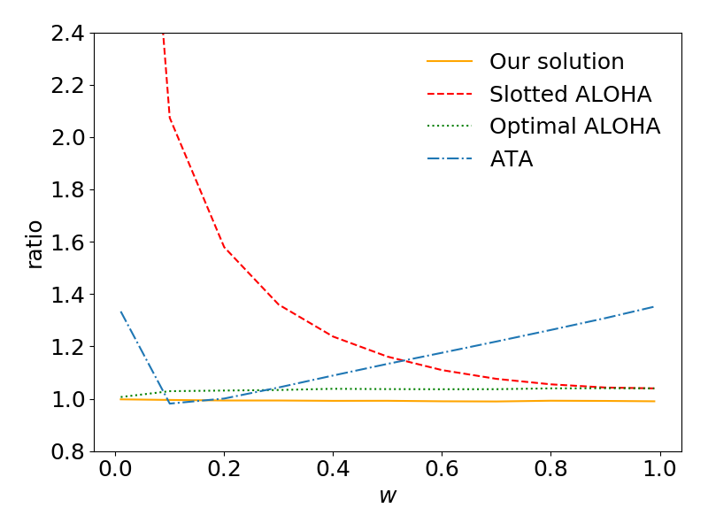
The results show that the average mismatches between theoretical $F(r,s)$ and actual $F(r,s)$ of our solution are about $0.7\%$ when $z=1$ and $12\%$ when $z=2$. Furthermore, we notice the actual value is always lower than theoretical value. These results indicate that our approximation is useful in practice.

Comparing the performance of different algorithms in Figure 2a and Figure 2b, we can observe that our strategy outperforms other three policies in all settings. Even when compared to the optimal ALOHA, which is not practical in real-world scenarios, our strategy shows a $4\%$ reduction when $z=1$ and a $9\%$ reduction when $z=2$. Additionally, the increase in the reduction of our strategy between $z=1$ and $z=2$ indicates that our strategy can better optimize the variance of AoI.

In Figure 2c and Figure 2d, we simulate $C=4$ to evaluate the performance of our strategy when the condition $N>C+4$ is not met. The Results indicate that our strategy outperforms the other three algorithms in nearly all settings, even when the condition $N>C+4$ is not satisfied.

This paper studies an optimization problem of moments of AoI for both active and passive users in a random access network. In this network, active users broadcast their transmissions following a Markov process and will interfere with each other. By applying a second-order model, we formulate moments of AoI as functions of state change probabilities in the Markov process. Next, we reveal the special properties of these functions and optimize moments of AoI for both active and passive users. The optimal solution indicates that the best strategy for active users is to become silent immediately after one transmission. Simulations show that this transmission strategy outperforms three baseline algorithms under various settings.

This material is based upon work supported in part by NSF under Award Number ECCS-2127721, in part by ARL and ARO under Grant Number W911NF-22-1-0151, and in part by ONR under Contract N00014-21-1-2385.

References

• [1] S. Kaul, R. Yates, and M. Gruteser, “Real-time status: How often should one update?,” in 2012 Proceedings IEEE INFOCOM, pp. 2731–2735, IEEE, 2012.
• [2] L. Huang and E. Modiano, “Optimizing age-of-information in a multi-class queueing system,” in 2015 IEEE international symposium on information theory (ISIT), pp. 1681–1685, IEEE, 2015.
• [3] K. Chen and L. Huang, “Age-of-information in the presence of error,” in 2016 IEEE International Symposium on Information Theory (ISIT), pp. 2579–2583, IEEE, 2016.
• [4] A. Kosta, N. Pappas, A. Ephremides, and V. Angelakis, “Age and value of information: Non-linear age case,” in 2017 IEEE International Symposium on Information Theory (ISIT), pp. 326–330, IEEE, 2017.
• [5] R. D. Yates and S. K. Kaul, “Status updates over unreliable multiaccess channels,” in 2017 IEEE International Symposium on Information Theory (ISIT), pp. 331–335, IEEE, 2017.
• [6] Y.-P. Hsu, E. Modiano, and L. Duan, “Age of information: Design and analysis of optimal scheduling algorithms,” in 2017 IEEE International Symposium on Information Theory (ISIT), pp. 561–565, IEEE, 2017.
• [7] I. Kadota, A. Sinha, E. Uysal-Biyikoglu, R. Singh, and E. Modiano, “Scheduling policies for minimizing age of information in broadcast wireless networks,” IEEE/ACM Transactions on Networking, vol. 26, no. 6, pp. 2637–2650, 2018.
• [8] R. D. Yates, “Status updates through networks of parallel servers,” in 2018 IEEE International Symposium on Information Theory (ISIT), pp. 2281–2285, IEEE, 2018.
• [9] Y. Sun, E. Uysal-Biyikoglu, and S. Kompella, “Age-optimal updates of multiple information flows,” in IEEE INFOCOM 2018-IEEE Conference on Computer Communications Workshops (INFOCOM WKSHPS), pp. 136–141, IEEE, 2018.
• [10] J. Sun, Z. Jiang, B. Krishnamachari, S. Zhou, and Z. Niu, “Closed-form whittle’s index-enabled random access for timely status update,” IEEE Transactions on Communications, vol. 68, no. 3, pp. 1538–1551, 2019.
• [11] A. Maatouk, S. Kriouile, M. Assaad, and A. Ephremides, “Asymptotically optimal scheduling policy for minimizing the age of information,” in 2020 IEEE International Symposium on Information Theory (ISIT), pp. 1747–1752, IEEE, 2020.
• [12] P. Zou, O. Ozel, and S. Subramaniam, “Optimizing information freshness through computation–transmission tradeoff and queue management in edge computing,” IEEE/ACM Transactions on Networking, vol. 29, no. 2, pp. 949–963, 2021.
• [13] A. Jaiswal and A. Chattopadhyay, “Minimization of age-of-information in remote sensing with energy harvesting,” in 2021 IEEE International Symposium on Information Theory (ISIT), pp. 3249–3254, IEEE, 2021.
• [14] R. D. Yates and S. K. Kaul, “Age of information in uncoordinated unslotted updating,” in 2020 IEEE International Symposium on Information Theory (ISIT), pp. 1759–1764, IEEE, 2020.
• [15] M. Moltafet, M. Leinonen, and M. Codreanu, “Average age of information for a multi-source m/m/1 queueing model with packet management,” in 2020 IEEE International Symposium on Information Theory (ISIT), pp. 1765–1769, IEEE, 2020.
• [16] C.-C. Wang, “How useful is delayed feedback in aoi minimization—a study on systems with queues in both forward and backward directions,” in 2022 IEEE International Symposium on Information Theory (ISIT), pp. 3192–3197, IEEE, 2022.
• [17] Y. Inoue, H. Masuyama, T. Takine, and T. Tanaka, “The stationary distribution of the age of information in fcfs single-server queues,” in 2017 IEEE International Symposium on Information Theory (ISIT), pp. 571–575, IEEE, 2017.
• [18] M. Moltafet, M. Leinonen, and M. Codreanu, “Aoi in source-aware preemptive m/g/1/1 queueing systems: Moment generating function,” in 2022 IEEE International Symposium on Information Theory (ISIT), pp. 139–143, IEEE, 2022.
• [19] M. Moltafet, M. Leinonen, and M. Codreanu, “Moment generating function of age of information in multisource m/g/1/1 queueing systems,” IEEE Transactions on Communications, vol. 70, no. 10, pp. 6503–6516, 2022.
• [20] S. Banerjee, R. Bhattacharjee, and A. Sinha, “Fundamental limits of age-of-information in stationary and non-stationary environments,” in 2020 IEEE International Symposium on Information Theory (ISIT), pp. 1741–1746, IEEE, 2020.
• [21] J. He, D. Zhang, S. Liu, Y. Zhou, and Y. Zhang, “Decentralized updates scheduling for data freshness in mobile edge computing,” in 2022 IEEE International Symposium on Information Theory (ISIT), pp. 3186–3191, IEEE, 2022.
• [22] X. Chen, K. Gatsis, H. Hassani, and S. S. Bidokhti, “Age of information in random access channels,” in 2020 IEEE International Symposium on Information Theory (ISIT), pp. 1770–1775, 2020.
• [23] H. Pan, T.-T. Chan, J. Li, and V. C. Leung, “Age of information with collision-resolution random access,” IEEE Transactions on Vehicular Technology, vol. 71, no. 10, pp. 11295–11300, 2022.
• [24] O. T. Yavascan and E. Uysal, “Analysis of slotted aloha with an age threshold,” IEEE Journal on Selected Areas in Communications, vol. 39, no. 5, pp. 1456–1470, 2021.
• [25] A. Munari, “Modern random access: An age of information perspective on irregular repetition slotted aloha,” IEEE Transactions on Communications, vol. 69, no. 6, pp. 3572–3585, 2021.
• [26] K. Saurav and R. Vaze, “Game of ages in a distributed network,” IEEE Journal on Selected Areas in Communications, vol. 39, no. 5, pp. 1240–1249, 2021.
• [27] H. H. Yang, C. Xu, X. Wang, D. Feng, and T. Q. Quek, “Understanding age of information in large-scale wireless networks,” IEEE Transactions on Wireless Communications, vol. 20, no. 5, pp. 3196–3210, 2021.
• [28] S. Kriouile and M. Assaad, “Minimizing the age of incorrect information for real-time tracking of markov remote sources,” in 2021 IEEE International Symposium on Information Theory (ISIT), pp. 2978–2983, IEEE, 2021.
• [29] X. Chen, R. Liu, S. Wang, and S. S. Bidokhti, “Timely broadcasting in erasure networks: Age-rate tradeoffs,” in 2021 IEEE International Symposium on Information Theory (ISIT), pp. 3127–3132, IEEE, 2021.
• [30] D. Guo, K. Nakhleh, I.-H. Hou, S. Kompella, and C. Kam, “A theory of second-order wireless network optimization and its application on aoi,” in IEEE INFOCOM 2022-IEEE Conference on Computer Communications, pp. 999–1008, IEEE, 2022.
• [31] G. Yao, A. Bedewy, and N. B. Shroff, “Age-optimal low-power status update over time-correlated fading channel,” IEEE Transactions on Mobile Computing, 2022.
• [32] A. Maatouk, M. Assaad, and A. Ephremides, “Analysis of an age-dependent stochastic hybrid system,” in 2022 IEEE International Symposium on Information Theory (ISIT), pp. 150–155, IEEE, 2022.
• [33] E. Schrödinger, “Zur theorie der fall-und steigversuche an teilchen mit brownscher bewegung,” Physikalische Zeitschrift, vol. 16, pp. 289–295, 1915.
• [34] J. L. Folks and R. S. Chhikara, “The inverse gaussian distribution and its statistical application—a review,” Journal of the Royal Statistical Society: Series B (Methodological), vol. 40, no. 3, pp. 263–275, 1978.
• [35] K. Krishnamoorthy, Handbook of statistical distributions with applications. Chapman and Hall/CRC, 2006.
-A Proof of Theorem 1
Let xn,tx_{n,t} be the indicator that the active user nn is in TX state in time slot tt.
First, we calculate the mean for active user nn in cluster cic_{i} and passive user jj. We have
ma\displaystyle m_{a} =Prob(xn,t=1)ζn,ζciProb(xζ,t=0)\displaystyle=Prob(x_{n,t}=1)\prod_{\zeta\neq n,\zeta\in c_{i}}Prob(x_{\zeta,t}=0)
=rr+s(sr+s)N1=λ(1λ)N1,\displaystyle=\frac{r}{r+s}\Big{(}\frac{s}{r+s}\Big{)}^{N-1}=\lambda(1-\lambda)^{N-1},
and mp=ζ=1CNProb(xζ,t=0)=(sr+s)CN=(1λ)CNm_{p}=\prod_{\zeta=1}^{CN}Prob(x_{\zeta,t}=0)=(\frac{s}{r+s})^{CN}=(1-\lambda)^{CN}.
Then, we derive the temporal variance for active user nn and passive user jj. According to the central limit theorem of Markov process, we have
va2\displaystyle v_{a}^{2} =Var(Sn(1))+2k=1Cov(Sn(1),Sn(k+1)),\displaystyle=Var(S_{n}(1))+2\sum_{k=1}^{\infty}Cov(S_{n}(1),S_{n}(k+1)),
vp2\displaystyle v_{p}^{2} =Var(Sj(1))+2k=1Cov(Sj(1),Sj(k+1)).\displaystyle=Var(S_{j}(1))+2\sum_{k=1}^{\infty}Cov(S_{j}(1),S_{j}(k+1)).
We first calculate va2v_{a}^{2}. Since Sn(1)S_{n}(1) is a Bernoulli random variable, it has
Var(Sn(1))=E[Sn(1)]E[Sn(1)]2=mama2\displaystyle Var(S_{n}(1))=E[S_{n}(1)]-E[S_{n}(1)]^{2}=m_{a}-m_{a}^{2}
Cov(Sn(1),Sn(k+1))\displaystyle Cov(S_{n}(1),S_{n}(k+1))
=E[Sn(1)Sn(k+1)]E[Sn(1)]E[Sn(k+1)]\displaystyle=E[S_{n}(1)S_{n}(k+1)]-E[S_{n}(1)]E[S_{n}(k+1)]
=(Prob(Sn(k+1)=1|Sn(1)=1)E[Sn(k+1)])E[Sn(1)]\displaystyle=(Prob(S_{n}(k+1)=1|S_{n}(1)=1)-E[S_{n}(k+1)])E[S_{n}(1)]
=(Prob(Sn(k+1)=1|Sn(1)=1)ma)ma.\displaystyle=(Prob(S_{n}(k+1)=1|S_{n}(1)=1)-m_{a})m_{a}.
Assume the active user nn is in cluster cic_{i}, we have Prob(Sn(k+1)=1|Sn(1)=1)=Prob(xn,k+1=1|Sn(1)=1)ζn,ζciProb(xζ,k+1=0|Sn(1)=1)Prob(S_{n}(k+1)=1|S_{n}(1)=1)=Prob(x_{n,k+1}=1|S_{n}(1)=1)\prod_{\zeta\neq n,\zeta\in c_{i}}Prob(x_{\zeta,k+1}=0|S_{n}(1)=1).
Let Gn,n(k)=Prob(xn,k=1|Sn(1)=1)G_{n,n}(k)=Prob(x_{n,k}=1|S_{n}(1)=1) and Gζ,n(k)=Prob(xζ,k=1|Sn(1)=1),ln,lciG_{\zeta,n}(k)=Prob(x_{\zeta,k}=1|S_{n}(1)=1),l\neq n,l\in c_{i}, we have Prob(Sn(k)=1|Sn(1)=1)=Gn,n(k)ζn,ζci(1Gζ,n(k))Prob(S_{n}(k)=1|S_{n}(1)=1)=G_{n,n}(k)\prod_{\zeta\neq n,\zeta\in c_{i}}(1-G_{\zeta,n}(k)) and
va2=\displaystyle v_{a}^{2}= 2k=1(Gn,n(k+1)ζn(1Gζ,n(k+1))ma)ma\displaystyle 2\sum_{k=1}^{\infty}(G_{n,n}(k+1)\prod_{\zeta\neq n}(1-G_{\zeta,n}(k+1))-m_{a})m_{a}
+mama2.\displaystyle+m_{a}-m_{a}^{2}.
Gn,n(k)G_{n,n}(k) can be calculated by
Gn,n(k)\displaystyle G_{n,n}(k) =Prob(xn,k=1|Sn(1)=1)\displaystyle=Prob(x_{n,k}=1|S_{n}(1)=1)
=Gn,n(k1)Prob(xn,k=1|xn,k1=1)\displaystyle=G_{n,n}(k-1)Prob(x_{n,k}=1|x_{n,k-1}=1)
+(1Gn,n(k1))Prob(xn,k=1|xn,k1=0)\displaystyle\quad+(1-G_{n,n}(k-1))Prob(x_{n,k}=1|x_{n,k-1}=0)
=Gn,n(k1)(1s)+(1Gn,n(k1))r\displaystyle=G_{n,n}(k-1)(1-s)+(1-G_{n,n}(k-1))r
=r+θGn,n(k1),\displaystyle=r+\theta G_{n,n}(k-1),
for k>1k>1, and Gn,n(1)=1G_{n,n}(1)=1. By i=2kθkiGn,n(i)\sum_{i=2}^{k}\theta^{k-i}G_{n,n}(i), we have
Gn,n(k)\displaystyle G_{n,n}(k) =i=2kθkir+θk1Gn,n(1)\displaystyle=\sum_{i=2}^{k}\theta^{k-i}r+\theta^{k-1}G_{n,n}(1)
=rr+s+sr+sθk1=λ+(1λ)θk1.\displaystyle=\frac{r}{r+s}+\frac{s}{r+s}\theta^{k-1}=\lambda+(1-\lambda)\theta^{k-1}.
For Gζ,n(k)G_{\zeta,n}(k), we also have
Gζ,n(k)\displaystyle G_{\zeta,n}(k) =Prob(xζ,k=1|Sn(1)=1)\displaystyle=Prob(x_{\zeta,k}=1|S_{n}(1)=1)
=Gζ,n(k1)Prob(xζ,k=1|xζ,k1=1)\displaystyle=G_{\zeta,n}(k-1)Prob(x_{\zeta,k}=1|x_{\zeta,k-1}=1)
+(1Gζ,n(k1))Prob(xζ,k=1|xζ,k1=0)\displaystyle\quad+(1-G_{\zeta,n}(k-1))Prob(x_{\zeta,k}=1|x_{\zeta,k-1}=0)
=Gζ,n(k1)(1s)+(1Gζ,n)(k1)r\displaystyle=G_{\zeta,n}(k-1)(1-s)+(1-G_{\zeta,n})(k-1)r
=r+θGζ,n(k1),\displaystyle=r+\theta G_{\zeta,n}(k-1),
for k>1k>1, and Gζ,n(1)=0G_{\zeta,n}(1)=0. Solving the recursive equation, we have Gζ,n(k)=λλθk1G_{\zeta,n}(k)=\lambda-\lambda\theta^{k-1}. Therefore,
va2=2k=1((λ+(1λ)θk)(1λ+λθk)N1ma)ma\displaystyle v_{a}^{2}=2\sum_{k=1}^{\infty}((\lambda+(1-\lambda)\theta^{k})(1-\lambda+\lambda\theta^{k})^{N-1}-m_{a})m_{a}
+mama2.\displaystyle\quad+m_{a}-m_{a}^{2}.
Now, we calculate vp2v_{p}^{2}. Sine Sj(1)S_{j}(1) is also a Bernoulli random variable in the system, we have
Var(Sj(1))=E[Sj(1)]E[Sj(1)]2=mpmp2\displaystyle Var(S_{j}(1))=E[S_{j}(1)]-E[S_{j}(1)]^{2}=m_{p}-m_{p}^{2}
Cov(Sj(1),Sj(k+1))\displaystyle Cov(S_{j}(1),S_{j}(k+1))
=E[Sj(1)Sj(k+1)]E[Sj(1)]E[Sj(k+1)]\displaystyle=E[S_{j}(1)S_{j}(k+1)]-E[S_{j}(1)]E[S_{j}(k+1)]
=(Prob(Sj(k+1)=1|Sj(1)=1)E[Sj(k+1)])E[Sj(1)]\displaystyle=(Prob(S_{j}(k+1)=1|S_{j}(1)=1)-E[S_{j}(k+1)])E[S_{j}(1)]
=(Prob(Sj(k+1)=1|Sj(1)=1)mp)mp.\displaystyle=(Prob(S_{j}(k+1)=1|S_{j}(1)=1)-m_{p})m_{p}.
Let Gn,j(k)=Prob(xn,k=1|Sj(1)=1)G_{n,j}(k)=Prob(x_{n,k}=1|S_{j}(1)=1), we have Prob(Sj(k+1)=1|Sj(1)=1)=n=1CN(1Gn,j(k))Prob(S_{j}(k+1)=1|S_{j}(1)=1)=\prod_{n=1}^{CN}(1-G_{n,j}(k)) and
vp2\displaystyle v_{p}^{2} =mpmp2+2k=1(n=1CN(1Gn,j(k+1))mp)mp.\displaystyle=m_{p}-m_{p}^{2}+2\sum_{k=1}^{\infty}(\prod_{n=1}^{CN}(1-G_{n,j}(k+1))-m_{p})m_{p}.
Gn,j(k)G_{n,j}(k) can be calculated by
Gn,j(k)\displaystyle G_{n,j}(k) =Prob(xn,k=1|Sj(1)=1)\displaystyle=Prob(x_{n,k}=1|S_{j}(1)=1)
=Gn,j(k1)Prob(xn,k=1|xn,k1=1)\displaystyle=G_{n,j}(k-1)Prob(x_{n,k}=1|x_{n,k-1}=1)
+(1Gn,j(k1))Prob(xn,k=1|xn,k1=0)\displaystyle\quad+(1-G_{n,j}(k-1))Prob(x_{n,k}=1|x_{n,k-1}=0)
=Gn,j(k1)(1s)+(1Gn,j)(k1)r\displaystyle=G_{n,j}(k-1)(1-s)+(1-G_{n,j})(k-1)r
=r+θGn,j(k1),\displaystyle=r+\theta G_{n,j}(k-1),
for k>1k>1, and Gn,j(1)=0G_{n,j}(1)=0. This expression is similar to that of Gζ,n(k)G_{\zeta,n}(k). Thus, solving the recursive equation, we have Gn,j(k)=λλθk1G_{n,j}(k)=\lambda-\lambda\theta^{k-1}. Thus,
vp2=2k=1((1λ+λθk)CNmp)mp+mpmp2.\displaystyle v_{p}^{2}=2\sum_{k=1}^{\infty}((1-\lambda+\lambda\theta^{k})^{CN}-m_{p})m_{p}+m_{p}-m_{p}^{2}.
-B Proof of Lemma 2
First, we show that we only need to consider the case θ0\theta\leq 0. The partial derivative of va2ma\frac{v_{a}^{2}}{m_{a}} with respect to θ\theta when λ\lambda is fixed is
va2θ\displaystyle\frac{\partial v_{a}^{2}}{\partial\theta} =2mak=1[(1λ)kθk1(1λ+λθk)N1\displaystyle=\frac{2}{m_{a}}\sum_{k=1}^{\infty}[(1-\lambda)k\theta^{k-1}(1-\lambda+\lambda\theta^{k})^{N-1}
+(λ+(1λ)θk)(N1)λkθk1(1λ+λθk)N2)]\displaystyle\quad+(\lambda+(1-\lambda)\theta^{k})(N-1)\lambda k\theta^{k-1}(1-\lambda+\lambda\theta^{k})^{N-2})]
=2mak=1[12λ+Nλ2+Nλ(1λ)θk]\displaystyle=\frac{2}{m_{a}}\sum_{k=1}^{\infty}[1-2\lambda+N\lambda^{2}+N\lambda(1-\lambda)\theta^{k}]
×kθk1(1λ+λθk)N2.\displaystyle\quad\times k\theta^{k-1}(1-\lambda+\lambda\theta^{k})^{N-2}.
When θ>0\theta>0, it is easy to verify that the partial derivative is positive. Similarly, we also have the partial derivative of vp2mp\frac{v_{p}^{2}}{m_{p}} with respect to θ\theta is positive when θ>0\theta>0. Thus, the optimal θ\theta is non-positive, and hence we only consider θ0\theta\leq 0 in the following proof.
We first prove (va2/ma2)λ0\frac{\partial(v_{a}^{2}/m_{a}^{2})}{\partial\lambda}\geq 0 when λ1N\lambda\geq\frac{1}{N}. Based on Theorem 1, we have
(va2/ma2)λ=2k=1[(1θk)(1λ+λθk)N1mama2\displaystyle\frac{\partial(v_{a}^{2}/m_{a}^{2})}{\partial\lambda}=2\sum_{k=1}^{\infty}\big{[}\frac{(1-\theta^{k})(1-\lambda+\lambda\theta^{k})^{N-1}m_{a}}{m_{a}^{2}}
+(λ+(1λ)θk)(N1)(1λ+λθk)N2(θk1)mama2\displaystyle+\frac{(\lambda+(1-\lambda)\theta^{k})(N-1)(1-\lambda+\lambda\theta^{k})^{N-2}(\theta^{k}-1)m_{a}}{m_{a}^{2}}
(1Nλ)(1λ)N2(λ+(1λ)θk)(1λ+λθk)N1ma2]\displaystyle-\frac{(1-N\lambda)(1-\lambda)^{N-2}(\lambda+(1-\lambda)\theta^{k})(1-\lambda+\lambda\theta^{k})^{N-1}}{m_{a}^{2}}\big{]}
(1Nλ)(1λ)N2ma2\displaystyle-\frac{(1-N\lambda)(1-\lambda)^{N-2}}{m_{a}^{2}}
=(Nλ1)(1λ)N2ma2+2k=1(1λ)N2(1λ+λθk)N2ma2\displaystyle=\frac{(N\lambda-1)(1-\lambda)^{N-2}}{m_{a}^{2}}+2\sum_{k=1}^{\infty}\frac{(1-\lambda)^{N-2}(1-\lambda+\lambda\theta^{k})^{N-2}}{m_{a}^{2}}
×θk[(N2)λ2(1λ)θk+(N2)λ2+2λ1].\displaystyle\times\theta^{k}\big{[}(N-2)\lambda^{2}(1-\lambda)\theta^{k}+(N-2)\lambda^{2}+2\lambda-1\big{]}.
Let ω(λ,θ,k,N):=(1λ)N2(1λ+λθk)N2θk[(N2)λ2(1λ)θk+(N2)λ2+2λ1]\omega(\lambda,\theta,k,N):=(1-\lambda)^{N-2}(1-\lambda+\lambda\theta^{k})^{N-2}\theta^{k}[(N-2)\lambda^{2}(1-\lambda)\theta^{k}+(N-2)\lambda^{2}+2\lambda-1] be the kk-th term in the above infinite summation. The following part is to prove k=1ξ(λ,θ,k,N)0\sum_{k=1}^{\infty}\xi(\lambda,\theta,k,N)\geq 0 or k=1ξ(λ,θ,k,N)+(Nλ1)0\sum_{k=1}^{\infty}\xi(\lambda,\theta,k,N)+(N\lambda-1)\geq 0.
Based on definition of λ\lambda and θ\theta, we first have (1λ)0(1-\lambda)\geq 0 and (1λ+λθk)0(1-\lambda+\lambda\theta^{k})\geq 0.
Consider the special case θ=1\theta=-1. θ=1\theta=-1 can only be achieved when λ=12\lambda=\frac{1}{2}. Thus, (1λ+λθk)N2(1-\lambda+\lambda\theta^{k})^{N-2} equals to 11 when kk is even, and equals to 0 when kk is odd. In this case, (N2)λ+2λ1>0(N-2)\lambda+2\lambda-1>0. Thus, ω(λ,θ,k,N)0\omega(\lambda,\theta,k,N)\geq 0 for any kk, and hence (va2/ma2)λ0\frac{\partial(v_{a}^{2}/m_{a}^{2})}{\partial\lambda}\geq 0.
Now, we discuss the case θ>1\theta>-1.
We first consider (N2)λ2+2λ10(N-2)\lambda^{2}+2\lambda-1\geq 0, which means λ[N11N2,1]\lambda\in[\frac{\sqrt{N-1}-1}{N-2},1]. In this case, [(N2)λ2(1λ)θk+(N2)λ2+2λ1][(N-2)\lambda^{2}(1-\lambda)\theta^{k}+(N-2)\lambda^{2}+2\lambda-1] is non-negative for all even kk, and is possible negative for odd kk (when kk is larger, equation becomes positive).
Consider kk from 22 to infinite, we compare the value with an even k=2qk=2q and its following odd k=2q+1k=2q+1. As θ(1,0]\theta\in(-1,0], we have |(1λ+λθ2q)N2|>|(1λ+λθ2q+1)N2||(1-\lambda+\lambda\theta^{2q})^{N-2}|>|(1-\lambda+\lambda\theta^{2q+1})^{N-2}| and |θ2q|>|θ2q+1||\theta^{2q}|>|\theta^{2q+1}|. Since θ0\theta\leq 0, when kk is even, we have θk0\theta^{k}\geq 0 and (N2)λ2(1λ)θk0(N-2)\lambda^{2}(1-\lambda)\theta^{k}\geq 0. When kk is odd, we have θk0\theta^{k}\leq 0 and (N2)λ2(1λ)θk0(N-2)\lambda^{2}(1-\lambda)\theta^{k}\leq 0. Hence, θk[(N2)λ2(1λ)θk+(N2)λ2+2λ1]θk[(N2)λ2+2λ1]\theta^{k}\big{[}(N-2)\lambda^{2}(1-\lambda)\theta^{k}+(N-2)\lambda^{2}+2\lambda-1\big{]}\geq\theta^{k}\big{[}(N-2)\lambda^{2}+2\lambda-1\big{]}, for all kk. Let ξ(k,λ,θ,N):=2(1λ+λθk)N2θk((N2)λ2+2λ1)\xi(k,\lambda,\theta,N):=2(1-\lambda+\lambda\theta^{k})^{N-2}\theta^{k}((N-2)\lambda^{2}+2\lambda-1). Based on above results, it is easy to verify ξ(2q,λ,θ,N)+ξ(2q+1,λ,θ,N)>0\xi(2q,\lambda,\theta,N)+\xi(2q+1,\lambda,\theta,N)>0, and hence k=2ξ(k,λ,θ,N)>0\sum_{k=2}^{\infty}\xi(k,\lambda,\theta,N)>0.
The remaining term is ξ(1,λ,θ,N)\xi(1,\lambda,\theta,N) and (Nλ1)(N\lambda-1). Summing them, denote ρ(θ,λ,N):=2θ[(N2)λ2(1+θ)(N2)λ3θ+2λ1]+Nλ1\rho(\theta,\lambda,N):=2\theta[(N-2)\lambda^{2}(1+\theta)-(N-2)\lambda^{3}\theta+2\lambda-1]+N\lambda-1, we have 2(1λ+λθ)N2θ[(N2)λ2(1+θ)(N2)λ3θ+2λ1]+Nλ1ρ(θ,λ,N)2(1-\lambda+\lambda\theta)^{N-2}\theta[(N-2)\lambda^{2}(1+\theta)-(N-2)\lambda^{3}\theta+2\lambda-1]+N\lambda-1\geq\rho(\theta,\lambda,N). The partial derivative of ρ(θ,λ,N)\rho(\theta,\lambda,N) with respect to θ\theta is ρ(θ,λ,N)θ=2[(N2)λ2(1+θ)(N2)λ3θ+2λ1]+2(N2)λ2(1λ)θ\frac{\partial\rho(\theta,\lambda,N)}{\partial\theta}=2[(N-2)\lambda^{2}(1+\theta)-(N-2)\lambda^{3}\theta+2\lambda-1]+2(N-2)\lambda^{2}(1-\lambda)\theta, which is an increasing function of θ\theta (convex function in θ(1,0)\theta\in(-1,0)). Choose θ=0\theta=0, ρ(θ,λ,N)θ|θ=0=2(N2)λ2+4λ2>0\frac{\partial\rho(\theta,\lambda,N)}{\partial\theta}|_{\theta=0}=2(N-2)\lambda^{2}+4\lambda-2>0 when λ[N11N2,1]\lambda\in[\frac{\sqrt{N-1}-1}{N-2},1]. Choosing θ=1\theta=-1, the partial derivative becomes ρ(θ,λ,N)θ|θ=1=4(N2)λ32(N2)λ2+4λ2\frac{\partial\rho(\theta,\lambda,N)}{\partial\theta}|_{\theta=-1}=4(N-2)\lambda^{3}-2(N-2)\lambda^{2}+4\lambda-2.
If ρ(θ,λ,N)θ|θ=1<0\frac{\partial\rho(\theta,\lambda,N)}{\partial\theta}|_{\theta=-1}<0, ρ(θ,λ,N)min{ρ(1,λ,N)+12ρ(θ,λ,N)θ|θ=1,ρ(0,λ,N)12ρ(θ,λ,N)θ|θ=0}\rho(\theta,\lambda,N)\geq\min\{\rho(-1,\lambda,N)+\frac{1}{2}\frac{\partial\rho(\theta,\lambda,N)}{\partial\theta}|_{\theta=-1},\rho(0,\lambda,N)-\frac{1}{2}\frac{\partial\rho(\theta,\lambda,N)}{\partial\theta}|_{\theta=0}\}. Note ρ(1,λ,N)+12ρ(θ,λ,N)θ|θ=1=2(N2)λ34λ+2+Nλ1+2(N2)λ3(N2)λ2+2λ1=(N2)λ(1λ)0\rho(-1,\lambda,N)+\frac{1}{2}\frac{\partial\rho(\theta,\lambda,N)}{\partial\theta}|_{\theta=-1}=-2(N-2)\lambda^{3}-4\lambda+2+N\lambda-1+2(N-2)\lambda^{3}-(N-2)\lambda^{2}+2\lambda-1=(N-2)\lambda(1-\lambda)\geq 0 and ρ(0,λ,N)12ρ(θ,λ,N)θ|θ=0=Nλ1(N2)λ22λ+1=(N2)λ(1λ)0\rho(0,\lambda,N)-\frac{1}{2}\frac{\partial\rho(\theta,\lambda,N)}{\partial\theta}|_{\theta=0}=N\lambda-1-(N-2)\lambda^{2}-2\lambda+1=(N-2)\lambda(1-\lambda)\geq 0. Thus, ρ(θ,λ,N)0\rho(\theta,\lambda,N)\geq 0 in this case.
If ρ(θ,λ,N)θ|θ=1=4(N2)λ32(N2)λ2+4λ2=2(2λ1)((N2)λ2+1)0\frac{\partial\rho(\theta,\lambda,N)}{\partial\theta}|_{\theta=-1}=4(N-2)\lambda^{3}-2(N-2)\lambda^{2}+4\lambda-2=2(2\lambda-1)((N-2)\lambda^{2}+1)\geq 0, the minimum ρ(θ,λ,N)\rho(\theta,\lambda,N) is achieved at smallest θ\theta and λ12\lambda\geq\frac{1}{2}. Since λ12\lambda\geq\frac{1}{2}, θ[λ1λ,0]\theta\in[\frac{\lambda-1}{\lambda},0], and hence ρ(θ,λ,N)ρ(λ1λ,λ,N)=2(λ1)(N2)λ2+6(N2)λ(λ1)2(N4)(λ1)2(λ1)λ+Nλ1\rho(\theta,\lambda,N)\geq\rho(\frac{\lambda-1}{\lambda},\lambda,N)=-2(\lambda-1)(N-2)\lambda^{2}+6(N-2)\lambda(\lambda-1)-2(N-4)(\lambda-1)-\frac{2(\lambda-1)}{\lambda}+N\lambda-1, and 2(λ1)λ2-\frac{2(\lambda-1)}{\lambda}\geq-2. Thus, ρ(θ,λ,N)2λ3(N2)+8(N2)λ2+(207N)λ+2N11\rho(\theta,\lambda,N)\geq-2\lambda^{3}(N-2)+8(N-2)\lambda^{2}+(20-7N)\lambda+2N-11. Taking derivative, we have 6(N2)λ2+16(N2)λ+207N-6(N-2)\lambda^{2}+16(N-2)\lambda+20-7N, which is positive when λ=1\lambda=1. The derivative of 6(N2)λ2+16(N2)λ+207N-6(N-2)\lambda^{2}+16(N-2)\lambda+20-7N is (N2)(1712λ)0(N-2)(17-12\lambda)\geq 0. Combined with λ[12,1]\lambda\in[\frac{1}{2},1], the value of 2λ3(N2)+8(N2)λ2+(207N)λ+2N112\lambda^{3}(N-2)+8(N-2)\lambda^{2}+(20-7N)\lambda+2N-11 is larger than the value of choosing λ=12\lambda=\frac{1}{2} (when N<30)N<30) or the value of λ=12\lambda=\frac{1}{2} plus the derivative at λ=12\lambda=\frac{1}{2} times 12\frac{1}{2} (when N30N\geq 30). The value at λ=12\lambda=\frac{1}{2} is 94N920\frac{9}{4}N-\frac{9}{2}\geq 0. When N30N\geq 30, the value of λ=12\lambda=\frac{1}{2} plus the derivative at λ=12\lambda=\frac{1}{2} times 12\frac{1}{2} is 2N+3>02N+3>0. Thus, ρ(θ,λ,N)0\rho(\theta,\lambda,N)\geq 0 in this case.
As ρ(θ,λ,N)0\rho(\theta,\lambda,N)\geq 0 in above all cases, and hence k=2ξ(k,λ,N)>0\sum_{k=2}^{\infty}\xi(k,\lambda,N)>0.
Next, we consider (N2)λ+2λ1<0(N-2)\lambda+2\lambda-1<0. Solving the inequation, we have λ[1N,N11N2)\lambda\in[\frac{1}{N},\frac{\sqrt{N-1}-1}{N-2}). Note when |(N2)λ2(1λ)θk||(N2)λ2+2λ1||(N-2)\lambda^{2}(1-\lambda)\theta^{k}|\geq|(N-2)\lambda^{2}+2\lambda-1|, θk((N2)λ2(1λ)θk+(N2)λ2+2λ1)0\theta^{k}((N-2)\lambda^{2}(1-\lambda)\theta^{k}+(N-2)\lambda^{2}+2\lambda-1)\geq 0 for both odd and even kk, and hence the summation is nonnegative for these kk. So, we only need to analyze the case |(N2)λ2(1λ)θk||(N2)λ2+2λ1||(N-2)\lambda^{2}(1-\lambda)\theta^{k}|\geq|(N-2)\lambda^{2}+2\lambda-1|, in which ω(λ,θ,k,N)0\omega(\lambda,\theta,k,N)\geq 0 when kk is odd and ω(λ,θ,k,N)0\omega(\lambda,\theta,k,N)\leq 0 when kk is even. Therefore, we consider ω(λ,θ,2q1,N)+ω(λ,θ,2q,N)\omega(\lambda,\theta,2q-1,N)+\omega(\lambda,\theta,2q,N). Note θ2q(N2)λ2+2λ1(N2)λ2(1λ)\theta^{2q}\leq-\frac{(N-2)\lambda^{2}+2\lambda-1}{(N-2)\lambda^{2}(1-\lambda)} in this case.
Recall the function ξ(k,λ,θ,N)\xi(k,\lambda,\theta,N), we have ω(λ,θ,2q1,N)+ω(λ,θ,2q,N)(1λ)N2ξ(2q1,λ,θ,N)+ξ(2q,λ,θ,N)=(1λ)N2θ2q1[(N2)λ2+2λ1][(1λ+λθ2q1)N2+θ(1λ+λθ2q)N2]\omega(\lambda,\theta,2q-1,N)+\omega(\lambda,\theta,2q,N)\geq(1-\lambda)^{N-2}\xi(2q-1,\lambda,\theta,N)+\xi(2q,\lambda,\theta,N)=(1-\lambda)^{N-2}\theta^{2q-1}[(N-2)\lambda^{2}+2\lambda-1][(1-\lambda+\lambda\theta^{2q-1})^{N-2}+\theta(1-\lambda+\lambda\theta^{2q})^{N-2}]. Note θ2q10\theta^{2q-1}\leq 0 and (N2)λ2+2λ10(N-2)\lambda^{2}+2\lambda-1\leq 0. The remaining is to compare (1λ+λθ2q1)N2(1-\lambda+\lambda\theta^{2q-1})^{N-2} and θ(1λ+λθ2q)N2-\theta(1-\lambda+\lambda\theta^{2q})^{N-2}. Divide these two terms, we have (1λ+λθ2q1)N2θ(1λ+λθ2q)N21θ(1λ+λθ11λ+λθ2)N2\frac{(1-\lambda+\lambda\theta^{2q-1})^{N-2}}{-\theta(1-\lambda+\lambda\theta^{2q})^{N-2}}\geq\frac{1}{-\theta}\big{(}\frac{1-\lambda+\lambda\theta^{1}}{1-\lambda+\lambda\theta^{2}}\big{)}^{N-2}.
When N13N\geq 13, we consider the bound θ[λ1λ,0]\theta\in[-\frac{\lambda}{1-\lambda},0] and λ[1N,N11N2]\lambda\in[\frac{1}{N},\frac{\sqrt{N-1}-1}{N-2}], and hence (1λ+λθ2q1)N2θ(1λ+λθ2q)N21λλ(1λλ2/(1λ)1λ+λ3/(1λ)2)N2=1λλ(13λ+2λ213λ+3λ2)N2=1λλ(111/λ23/λ+3)N2\frac{(1-\lambda+\lambda\theta^{2q-1})^{N-2}}{-\theta(1-\lambda+\lambda\theta^{2q})^{N-2}}\geq\frac{1-\lambda}{\lambda}(\frac{1-\lambda-\lambda^{2}/(1-\lambda)}{1-\lambda+\lambda^{3}/(1-\lambda)^{2}})^{N-2}=\frac{1-\lambda}{\lambda}(\frac{1-3\lambda+2\lambda^{2}}{1-3\lambda+3\lambda^{2}})^{N-2}=\frac{1-\lambda}{\lambda}(1-\frac{1}{1/\lambda^{2}-3/\lambda+3})^{N-2}. By doing the partial derivative with respect to λ\lambda, we have (1λ)/λλ=1λ2<0\frac{\partial(1-\lambda)/\lambda}{\partial\lambda}=\frac{-1}{\lambda^{2}}<0 and (1/λ23/λ)λ=1/λ3(3λ2)<0\frac{\partial(1/\lambda^{2}-3/\lambda)}{\partial\lambda}=1/\lambda^{3}(3\lambda-2)<0 when λ[1N,N11N2]\lambda\in[\frac{1}{N},\frac{\sqrt{N-1}-1}{N-2}]. Thus, 1λλ(111/λ23/λ+3)N2\frac{1-\lambda}{\lambda}(1-\frac{1}{1/\lambda^{2}-3/\lambda+3})^{N-2} is a decreasing function of λ\lambda. Taking λ=N11N2\lambda=\frac{\sqrt{N-1}-1}{N-2} into this function, we obtain the lower bound, which is a function of only one variable NN. By doing the partial derivative, it can be verified that it is an increasing function of NN. Taking N=13N=13, we can verify 1λλ(111/λ23/λ+3)N21\frac{1-\lambda}{\lambda}(1-\frac{1}{1/\lambda^{2}-3/\lambda+3})^{N-2}\geq 1. Hence (1λ+λθ2q1)N2θ(1λ+λθ2q)N21\frac{(1-\lambda+\lambda\theta^{2q-1})^{N-2}}{-\theta(1-\lambda+\lambda\theta^{2q})^{N-2}}\geq 1 for N13N\geq 13.
When N<13N<13, we should consider both bound for θ\theta, θ[λ1λ,0]\theta\in[-\frac{\lambda}{1-\lambda},0] and θ2q(N2)λ2+2λ1(N2)λ2(1λ)\theta^{2q}\leq-\frac{(N-2)\lambda^{2}+2\lambda-1}{(N-2)\lambda^{2}(1-\lambda)}, which comes from the inequation condition θk((N2)λ2(1λ)θ2i+(N2)λ2+2λ1)0\theta^{k}((N-2)\lambda^{2}(1-\lambda)\theta^{2i}+(N-2)\lambda^{2}+2\lambda-1)\leq 0. For λ\lambda, we separate its domain to be [1N,Γ][\frac{1}{N},\Gamma] and [Γ,N11N2][\Gamma,\frac{\sqrt{N-1}-1}{N-2}], where Γ=0.031N+0.97N11N2\Gamma=0.03*\frac{1}{N}+0.97*\frac{\sqrt{N-1}-1}{N-2}. It can be verified that, when λ[1N,Γ]\lambda\in[\frac{1}{N},\Gamma], 1λλ(111/λ23/λ+3)N21\frac{1-\lambda}{\lambda}(1-\frac{1}{1/\lambda^{2}-3/\lambda+3})^{N-2}\geq 1 for every NN that N<13N<13, using the same strategy as that for N13N\geq 13 and the only change is the upper bound for λ\lambda. When λ[Γ,N11N2]\lambda\in[\Gamma,\frac{\sqrt{N-1}-1}{N-2}], we analyze the sign of (1λ+λθ2q1)N2+θ(1λ+λθ2q)N2(1-\lambda+\lambda\theta^{2q-1})^{N-2}+\theta(1-\lambda+\lambda\theta^{2q})^{N-2}. Since θ2q(N2)λ2+2λ1(N2)λ2(1λ)\theta^{2q}\leq-\frac{(N-2)\lambda^{2}+2\lambda-1}{(N-2)\lambda^{2}(1-\lambda)}, by doing the partial derivative, the upper bound of θ2q\theta^{2q} is a decreasing function of λ\lambda. Hence, the maximum θ2q\theta^{2q} is achieved when λ=Γ\lambda=\Gamma and then θ2qγ\theta^{2q}\leq-\gamma, where γ=(N2)Γ2+2th1(N2)Γ2(1Γ)\gamma=\frac{(N-2)\Gamma^{2}+2th-1}{(N-2)\Gamma^{2}(1-\Gamma)} is a variable only related to NN. Thus, (1λ+λθ2q1)N2+θ(1λ+λθ2q)N2(1λλγ)N2γ(1λ+λγ)N2(1-\lambda+\lambda\theta^{2q-1})^{N-2}+\theta(1-\lambda+\lambda\theta^{2q})^{N-2}\geq(1-\lambda-\lambda\sqrt{\gamma})^{N-2}-\sqrt{\gamma}(1-\lambda+\lambda\gamma)^{N-2}, which, verified by doing partial derivative, is a decreasing function of λ\lambda. Then, taking λ=N11N2\lambda=\frac{\sqrt{N-1}-1}{N-2}, we can verify that (1λλγ)N2γ(1λ+λγ)N20(1-\lambda-\lambda\sqrt{\gamma})^{N-2}-\sqrt{\gamma}(1-\lambda+\lambda\gamma)^{N-2}\geq 0 for every NN that N<13N<13. Therefore, (1λ+λθ2q1)N2+θ(1λ+λθ2q)N20(1-\lambda+\lambda\theta^{2q-1})^{N-2}+\theta(1-\lambda+\lambda\theta^{2q})^{N-2}\geq 0 when N<13N<13
As (1λ+λθ2q1)N2+θ(1λ+λθ2q)N20(1-\lambda+\lambda\theta^{2q-1})^{N-2}+\theta(1-\lambda+\lambda\theta^{2q})^{N-2}\geq 0 for both N13N\geq 13 and N<13N<13, ω(λ,θ,2q1,N)+ω(λ,θ,2q,N)0\omega(\lambda,\theta,2q-1,N)+\omega(\lambda,\theta,2q,N)\geq 0, and hence k=1ξ(k,λ,θ,N)0\sum_{k=1}^{\infty}\xi(k,\lambda,\theta,N)\geq 0 when (N2)λ+2λ1<0(N-2)\lambda+2\lambda-1<0.
Since k=1ξ(k,λ,θ,N)0\sum_{k=1}^{\infty}\xi(k,\lambda,\theta,N)\geq 0 when (N2)λ+2λ1<0(N-2)\lambda+2\lambda-1<0 and k=1ξ(k,λ,θ,N)+Nλ10\sum_{k=1}^{\infty}\xi(k,\lambda,\theta,N)+N\lambda-1\geq 0 when (N2)λ+2λ10(N-2)\lambda+2\lambda-1\geq 0, we have, when λ1N\lambda\geq\frac{1}{N},
(va2/ma2)λ0,\displaystyle\frac{\partial(v_{a}^{2}/m_{a}^{2})}{\partial\lambda}\geq 0,
Now, we discuss passive users. Based on Theorem 1, we have
(vp2/mp2)λ=2k=1[CN(θk1)(1λ+λθk)CN1mpmp2\displaystyle\frac{\partial(v_{p}^{2}/m_{p}^{2})}{\partial\lambda}=2\sum_{k=1}^{\infty}\Big{[}\frac{CN(\theta^{k}-1)(1-\lambda+\lambda\theta^{k})^{CN-1}m_{p}}{m_{p}^{2}}
+CN(1λ)CN1(1λ+λθk)CNmp2]+CN(1λ)CNmp2\displaystyle+\frac{CN(1-\lambda)^{CN-1}(1-\lambda+\lambda\theta^{k})^{CN}}{m_{p}^{2}}\Big{]}+\frac{CN(1-\lambda)^{CN}}{m_{p}^{2}}
=2CN(1λ)CN1[1λ+k=1(1λ+λθk)CN1θk]mp2.\displaystyle=\frac{2CN(1-\lambda)^{CN-1}[1-\lambda+\sum_{k=1}^{\infty}(1-\lambda+\lambda\theta^{k})^{CN-1}\theta^{k}]}{m_{p}^{2}}.
Since θ(1,0)\theta\in(-1,0) and 1λ+λθk01-\lambda+\lambda\theta^{k}\geq 0 for all kk,
(vp2/mp2)λ\displaystyle\frac{\partial(v_{p}^{2}/m_{p}^{2})}{\partial\lambda}
2CN(1λ)CN1[1λ+k=1(1λ)CN1θk]mp2\displaystyle\geq\frac{2CN(1-\lambda)^{CN-1}[1-\lambda+\sum_{k=1}^{\infty}(1-\lambda)^{CN-1}\theta^{k}]}{m_{p}^{2}}
=CN(1λ)CN1[1λ+(1λ)CN1θ1θ]mp2.\displaystyle=\frac{CN(1-\lambda)^{CN-1}[1-\lambda+(1-\lambda)^{CN-1}\frac{\theta}{1-\theta}]}{m_{p}^{2}}.
When λ[0,12]\lambda\in[0,\frac{1}{2}], θ[λ1λ,0]\theta\in[-\frac{\lambda}{1-\lambda},0], and hence
(vp2/mp2)λ2CN(1λ)CN1[1λ(1λ)CN1λ]mp2\displaystyle\frac{\partial(v_{p}^{2}/m_{p}^{2})}{\partial\lambda}\geq\frac{2CN(1-\lambda)^{CN-1}[1-\lambda-(1-\lambda)^{CN-1}\lambda]}{m_{p}^{2}}
=2CN(1λ)CN1[1(1+(1λ)CN1)λ]mp2\displaystyle=\frac{2CN(1-\lambda)^{CN-1}[1-(1+(1-\lambda)^{CN-1})\lambda]}{m_{p}^{2}}
2CN(1λ)CN1[1(1+1)12]mp2=0.\displaystyle\geq\frac{2CN(1-\lambda)^{CN-1}[1-(1+1)\frac{1}{2}]}{m_{p}^{2}}=0.
When λ[12,1]\lambda\in[\frac{1}{2},1], θ[λ1λ,0]\theta\in[\frac{\lambda-1}{\lambda},0], and then
(vp2/mp2)λ2CN(1λ)CN1[1λ(1λ)CN]mp2\displaystyle\frac{\partial(v_{p}^{2}/m_{p}^{2})}{\partial\lambda}\geq\frac{2CN(1-\lambda)^{CN-1}[1-\lambda-(1-\lambda)^{CN}]}{m_{p}^{2}}
2CN(1λ)CN1[1λ(1λ)]mp2=0.\displaystyle\geq\frac{2CN(1-\lambda)^{CN-1}[1-\lambda-(1-\lambda)]}{m_{p}^{2}}=0.
Therefore, when λ1N\lambda\geq\frac{1}{N},
(vp2/mp2)λ0.\displaystyle\frac{\partial(v_{p}^{2}/m_{p}^{2})}{\partial\lambda}\geq 0.
-C Proof of Lemma 3
The partial derivative of va2v_{a}^{2} with respect to θ\theta when λ\lambda is determined is
va2θ=2mak=1[(1λ)kθk1(1λ+λθk)N1\displaystyle\frac{\partial v_{a}^{2}}{\partial\theta}=2m_{a}\sum_{k=1}^{\infty}[(1-\lambda)k\theta^{k-1}(1-\lambda+\lambda\theta^{k})^{N-1}
=\displaystyle= 2mak=1[12λ+Nλ2+Nλ(1λ)θk]\displaystyle 2m_{a}\sum_{k=1}^{\infty}[1-2\lambda+N\lambda^{2}+N\lambda(1-\lambda)\theta^{k}]
Let ψ(k):=2ma[12λ+Nλ2+Nλ(1λ)θk]kθk1(1λ+λθk)N2\psi(k):=2m_{a}[1-2\lambda+N\lambda^{2}+N\lambda(1-\lambda)\theta^{k}]k\theta^{k-1}(1-\lambda+\lambda\theta^{k})^{N-2} be the kkth term in the above equation.
We first show that α,β<12\alpha,\beta<\frac{1}{2}. Choosing y=0y=0 and y=12y=\frac{1}{2}, we have hN(0)=h¯N(0)=1h_{N}(0)=\bar{h}_{N}(0)=1, hN(12)=38N+112<0h_{N}(\frac{1}{2})=-\frac{3}{8}N+\frac{1}{12}<0 and h¯N(12)=18N<0\bar{h}_{N}(\frac{1}{2})=-\frac{1}{8}N<0. Therefore, there must exists one root that in (0,12)(0,\frac{1}{2}) for both hN(y)h_{N}(y) and h¯N(y)\bar{h}_{N}(y). Thus, λ[0,12)\lambda\in[0,\frac{1}{2}) and hence θ[λ1λ,1]\theta\in[-\frac{\lambda}{1-\lambda},1].
Therefore, [12λ+Nλ2+Nλ(1λ)θk]12×12+Nλ2Nλ(1λ)λ1λ=0[1-2\lambda+N\lambda^{2}+N\lambda(1-\lambda)\theta^{k}]\geq 1-2\times\frac{1}{2}+N\lambda^{2}-N\lambda(1-\lambda)\frac{\lambda}{1-\lambda}=0, and 1λ+λθk1λ+λθ11λλλ1λ>12λ01-\lambda+\lambda\theta^{k}\geq 1-\lambda+\lambda\theta^{1}\geq 1-\lambda-\lambda\frac{\lambda}{1-\lambda}>1-2\lambda\geq 0. So, ψ(k)<0\psi(k)<0 only when θ<0\theta<0 and kk is even.
The expression of ψ(2i1)ψ(2i)\frac{\psi(2i-1)}{\psi(2i)} is
ψ(2i1)ψ(2i)=\displaystyle-\frac{\psi(2i-1)}{\psi(2i)}= 12λ+Nλ2+Nλ(1λ)θ2i112λ+Nλ2+Nλ(1λ)θ2i2i12i\displaystyle-\frac{1-2\lambda+N\lambda^{2}+N\lambda(1-\lambda)\theta^{2i-1}}{1-2\lambda+N\lambda^{2}+N\lambda(1-\lambda)\theta^{2i}}\frac{2i-1}{2i}
×θ2i1θ2i(1λ+λθ2i11λ+λθ2i)N2.\displaystyle\times\frac{\theta^{2i-1}}{\theta^{2i}}\Big{(}\frac{1-\lambda+\lambda\theta^{2i-1}}{1-\lambda+\lambda\theta^{2i}}\Big{)}^{N-2}.
When θ0\theta\geq 0, it is easy to verify that ψ(2i1)ψ(2i)1-\frac{\psi(2i-1)}{\psi(2i)}\geq 1 since θ1\theta\leq 1.
When λ1λθ<0\frac{-\lambda}{1-\lambda}\leq\theta<0, we have
ψ(2i1)ψ(2i)12λ+Nλ2+Nλ(1λ)θ112λ+Nλ2+Nλ(1λ)θ212θ1θ2\displaystyle\frac{\psi(2i-1)}{\psi(2i)}\geq\frac{1-2\lambda+N\lambda^{2}+N\lambda(1-\lambda)\theta^{1}}{1-2\lambda+N\lambda^{2}+N\lambda(1-\lambda)\theta^{2}}\frac{1}{2}\frac{\theta^{1}}{\theta^{2}}
×(1λ+λθ11λ+λθ2)N2\displaystyle\quad\times\Big{(}\frac{1-\lambda+\lambda\theta^{1}}{1-\lambda+\lambda\theta^{2}}\Big{)}^{N-2}
12λ+Nλ2Nλ(1λ)λ1λ12λ+Nλ2+Nλ(1λ)λ2(1λ)2121λλ\displaystyle\geq\frac{1-2\lambda+N\lambda^{2}-N\lambda(1-\lambda)\frac{\lambda}{1-\lambda}}{1-2\lambda+N\lambda^{2}+N\lambda(1-\lambda)\frac{\lambda^{2}}{(1-\lambda)^{2}}}\frac{1}{2}\frac{1-\lambda}{\lambda}
×(1λλλ1λ1λ+λλ2(1λ)2)N2\displaystyle\quad\times\Big{(}\frac{1-\lambda-\lambda\frac{\lambda}{1-\lambda}}{1-\lambda+\lambda\frac{\lambda^{2}}{(1-\lambda)^{2}}}\Big{)}^{N-2}
=1λ2λ13λ+2λ213λ+(N+2)λ2(1λ213λ+3λ2)N2.\displaystyle=\frac{1-\lambda}{2\lambda}\frac{1-3\lambda+2\lambda^{2}}{1-3\lambda+(N+2)\lambda^{2}}(1-\frac{\lambda^{2}}{1-3\lambda+3\lambda^{2}})^{N-2}.
Define AN(y),B¯(y)A_{N}(y),\bar{B}(y) and CN(y)C_{N}(y) as follows:
AN(y)\displaystyle A_{N}(y) =13y+2y213y+(N+2)y2(1y213y+3y2)N2,\displaystyle=\frac{1-3y+2y^{2}}{1-3y+(N+2)y^{2}}(1-\frac{y^{2}}{1-3y+3y^{2}})^{N-2},
B¯(y)\displaystyle\bar{B}(y) =2y1y,CN(y)=13y(N4)y213y+(N+2)y2.\displaystyle=\frac{2y}{1-y},\quad C_{N}(y)=\frac{1-3y-(N-4)y^{2}}{1-3y+(N+2)y^{2}}.
Then, ψ(2i1)ψ(2i)AN(y)B¯(y)\frac{\psi(2i-1)}{\psi(2i)}\geq\frac{A_{N}(y)}{\bar{B}(y)}.
First, we prove CN(y)B¯(y)C_{N}(y)\geq\bar{B}(y). Subtracting B¯(y)\bar{B}(y) from CN(y)C_{N}(y), we have
CN(y)B¯(y)=13y(N4)y213y+(N+2)y22y1y\displaystyle C_{N}(y)-\bar{B}(y)=\frac{1-3y-(N-4)y^{2}}{1-3y+(N+2)y^{2}}-\frac{2y}{1-y}
=(13y)2(1y)(N4)y22y(N+2)y2(13y+(N+2)y2)(1y)\displaystyle=\frac{(1-3y)^{2}-(1-y)(N-4)y^{2}-2y(N+2)y^{2}}{(1-3y+(N+2)y^{2})(1-y)}
=hN(y)(13y+(N+2)y2)(1y).\displaystyle=\frac{h_{N}(y)}{(1-3y+(N+2)y^{2})(1-y)}.
As α\alpha is the smallest positive root of hN(y)h_{N}(y) and hN(0)=1>0h_{N}(0)=1>0, hN(y)0h_{N}(y)\geq 0 when y[0,α]y\in[0,\alpha]. Note α<12\alpha<\frac{1}{2}.
Now we check whether (13y+(N+2)y2)(1-3y+(N+2)y^{2}) is positive. The derivative of (13y+(N+2)y2)(1-3y+(N+2)y^{2}) is 2(N+2)y32(N+2)y-3 and hence it achieves minimum when y=32(N+2)y=\frac{3}{2(N+2)}. Choosing y=32(N+2)y=\frac{3}{2(N+2)}, we have (13y+(N+2)y2)=192(N+2)+94(N+2)=194(N+2)194(2+2)>0(1-3y+(N+2)y^{2})=1-\frac{9}{2(N+2)}+\frac{9}{4(N+2)}=1-\frac{9}{4(N+2)}\geq 1-\frac{9}{4(2+2)}>0.
Since (13y+(N+2)y2)(1-3y+(N+2)y^{2}), (1y)(1-y) and h¯N(y)\bar{h}_{N}(y) are all non-negative when y[0,α]y\in[0,\alpha], we have
CN(y)B¯(y)=hN(y)(13y+(N+2)y2)(1y)0.\displaystyle C_{N}(y)-\bar{B}(y)=\frac{h_{N}(y)}{(1-3y+(N+2)y^{2})(1-y)}\geq 0.
Next, we prove AN(y)CN(y)A_{N}(y)\geq C_{N}(y).
We know that (1y)N1Ny(1-y)^{N}\approx 1-Ny from binomial approximation. Let j(y)=(1y)N(1Ny)j(y)=(1-y)^{N}-(1-Ny). The derivative of j(y)j(y) is N[1(1y)N1]N[1-(1-y)^{N-1}]. As (1y)N11(1-y)^{N-1}\leq 1 when 0y10\leq y\leq 1, we have j(y)j(y) is increasing when y[0,1]y\in[0,1]. Hence, j(y)j(0)=0j(y)\geq j(0)=0, which means (1y)N1Ny(1-y)^{N}\geq 1-Ny, when y[0,1]y\in[0,1].
Now, we want to find whether y23y23y+1\frac{y^{2}}{3y^{2}-3y+1} is between 0 and 11. The derivative of 3y23y+1y23y^{2}-3y+1-y^{2} is 4y34y-3. Thus, when 0y120\leq y\leq\frac{1}{2}, 3y23y+1y23×143×12+114=03y^{2}-3y+1-y^{2}\geq 3\times\frac{1}{4}-3\times\frac{1}{2}+1-\frac{1}{4}=0. Therefore, 3y23y+1y23y^{2}-3y+1\geq y^{2}. As 3y23y+1>03y^{2}-3y+1>0 and y20y^{2}\geq 0, we have y23y23y+11\frac{y^{2}}{3y^{2}-3y+1}\leq 1 and y23y23y+10\frac{y^{2}}{3y^{2}-3y+1}\geq 0 when y[0,12]y\in[0,\frac{1}{2}].
Thus, when y[0,12]y\in[0,\frac{1}{2}],
(1y23y23y+1)N21(N2)y23y23y+1.\displaystyle(1-\frac{y^{2}}{3y^{2}-3y+1})^{N-2}\geq 1-(N-2)\frac{y^{2}}{3y^{2}-3y+1}.
Then,
AN(y)\displaystyle A_{N}(y) =13y+2y213y+(N+2)y2(1y213y+3y2)N2\displaystyle=\frac{1-3y+2y^{2}}{1-3y+(N+2)y^{2}}(1-\frac{y^{2}}{1-3y+3y^{2}})^{N-2}
13y+2y213y+(N+2)y2[1(N2)y213y+3y2]\displaystyle\geq\frac{1-3y+2y^{2}}{1-3y+(N+2)y^{2}}[1-(N-2)\frac{y^{2}}{1-3y+3y^{2}}]
=13y+2y213y+(N+2)y213y(N5)y213y+3y2.\displaystyle=\frac{1-3y+2y^{2}}{1-3y+(N+2)y^{2}}\frac{1-3y-(N-5)y^{2}}{1-3y+3y^{2}}.
When N2N\geq 2, 13y(N5)y213y+3y21-3y-(N-5)y^{2}\leq 1-3y+3y^{2}, and hence
13y(N5)y213y+3y213y(N4)y213y+2y2.\displaystyle\frac{1-3y-(N-5)y^{2}}{1-3y+3y^{2}}\geq\frac{1-3y-(N-4)y^{2}}{1-3y+2y^{2}}.
Therefore,
AN(y)\displaystyle A_{N}(y) 13y+2y213y+(N+2)y213y(N4)y213y+2y2\displaystyle\geq\frac{1-3y+2y^{2}}{1-3y+(N+2)y^{2}}\frac{1-3y-(N-4)y^{2}}{1-3y+2y^{2}}
=13y(N4)y213y+(N+2)y2=CN(y).\displaystyle=\frac{1-3y-(N-4)y^{2}}{1-3y+(N+2)y^{2}}=C_{N}(y).
So, when y[0,α]y\in[0,\alpha], AN(y)CN(y)B¯(y)A_{N}(y)\geq C_{N}(y)\geq\bar{B}(y). Thus,
ψ(2i1)ψ(2i)AN(λ)B¯(λ)1.\displaystyle\frac{\psi(2i-1)}{\psi(2i)}\geq\frac{A_{N}(\lambda)}{\bar{B}(\lambda)}\geq 1.
Hence, va2θ0\frac{\partial v_{a}^{2}}{\partial\theta}\geq 0 and va2v_{a}^{2} achieves its minimum value when θ\theta is minimized. Thus, choosing r=λ1λr=\frac{\lambda}{1-\lambda} and s=1s=1 minimizes va2v_{a}^{2}.
Since E[AoIaz]E[AoI_{a}^{z}] is an increasing function of va2v_{a}^{2}, choosing r=λ1λr=\frac{\lambda}{1-\lambda} and s=1s=1 also minimizes E[AoIaz]E[AoI_{a}^{z}].
Next, we consider passive users.
Recall the expression of vp2v_{p}^{2},
vp2\displaystyle v_{p}^{2} =2k=1((1λ+λθk)CNmp)mp+mpmp2.\displaystyle=2\sum_{k=1}^{\infty}((1-\lambda+\lambda\theta^{k})^{CN}-m_{p})m_{p}+m_{p}-m_{p}^{2}.
For this expression, it is easy to verify that vp2|θ>0vp2|θ=0v_{p}^{2}|_{\theta>0}\geq v_{p}^{2}|_{\theta=0}. Therefore, vp2v_{p}^{2} reaches its minimum in the region λ1λθ0-\frac{\lambda}{1-\lambda}\leq\theta\leq 0.
The partial derivative of vp2v_{p}^{2} with respect to θ\theta is
vp2θ=2mpk=1CNkλθk1(1λ+λθk)CN1.\displaystyle\frac{\partial v_{p}^{2}}{\partial\theta}=2m_{p}\sum_{k=1}^{\infty}CNk\lambda\theta^{k-1}(1-\lambda+\lambda\theta^{k})^{CN-1}.
Let ϕ(k)=2mpCNkλθk1(1λ+λθk)CN1\phi(k)=2m_{p}CNk\lambda\theta^{k-1}(1-\lambda+\lambda\theta^{k})^{CN-1} be the kthk-th term of the partial derivative above. When θ[λ1λ,0]\theta\in[-\frac{\lambda}{1-\lambda},0], we can find that ϕ(k)0\phi(k)\geq 0 when kk is odd and ϕ(k)<0\phi(k)<0 when kk is even. Thus, vp2θ\frac{\partial v_{p}^{2}}{\partial\theta} is positive if ϕ(2i1)ϕ(2i)>1-\frac{\phi(2i-1)}{\phi(2i)}>1 for all positive integer ii.
Plugging in the formula of ϕ(k)\phi(k),
ϕ(2i1)ϕ(2i)=2i12i1θ(1λ+λθ2i11λ+λθ2i)CN1.\displaystyle-\frac{\phi(2i-1)}{\phi(2i)}=-\frac{2i-1}{2i}\frac{1}{\theta}\Big{(}\frac{1-\lambda+\lambda\theta^{2i-1}}{1-\lambda+\lambda\theta^{2i}}\Big{)}^{CN-1}.
Since θ2i1θλ1λ\theta^{2i-1}\geq\theta\geq-\frac{\lambda}{1-\lambda} and θ2iθ2λ2(1λ)2\theta^{2i}\leq\theta^{2}\leq\frac{\lambda^{2}}{(1-\lambda)^{2}} when θ[λ1λ,0]\theta\in[-\frac{\lambda}{1-\lambda},0], we have
ϕ(2i1)ϕ(2i)\displaystyle-\frac{\phi(2i-1)}{\phi(2i)} ϕ(1)ϕ(2)=121θ(1λ+λθ1λ+λθ2)CN1\displaystyle\geq-\frac{\phi(1)}{\phi(2)}=-\frac{1}{2}\frac{1}{\theta}\Big{(}\frac{1-\lambda+\lambda\theta}{1-\lambda+\lambda\theta^{2}}\Big{)}^{CN-1}
1λ2λ(1λ23λ23λ+1)CN1.\displaystyle\geq\frac{1-\lambda}{2\lambda}\Big{(}1-\frac{\lambda^{2}}{3\lambda^{2}-3\lambda+1}\Big{)}^{CN-1}.
Define A¯CN(y)\bar{A}_{CN}(y) as follows.
A¯CN(y)\displaystyle\bar{A}_{CN}(y) =(1y23y23y+1)CN1.\displaystyle=\Big{(}1-\frac{y^{2}}{3y^{2}-3y+1}\Big{)}^{CN-1}.
When y[0,12]y\in[0,\frac{1}{2}],
A¯CN(y)B¯(y)=(1y23y23y+1)CN12y1y\displaystyle\bar{A}_{CN}(y)-\bar{B}(y)=\Big{(}1-\frac{y^{2}}{3y^{2}-3y+1}\Big{)}^{CN-1}-\frac{2y}{1-y}
1(CN1)y23y23y+12y1y\displaystyle\geq 1-(CN-1)\frac{y^{2}}{3y^{2}-3y+1}-\frac{2y}{1-y}
=h¯CN(y)(3y23y+1)(1y).\displaystyle=\frac{\bar{h}_{CN}(y)}{(3y^{2}-3y+1)(1-y)}.
Note h¯CN(0)=1\bar{h}_{CN}(0)=1, h¯CN(12)=CN8\bar{h}_{CN}(\frac{1}{2})=-\frac{CN}{8}, and β\beta is the smallest positive root of h¯CN(y)\bar{h}_{CN}(y). Thus, h¯CN(y)0\bar{h}_{CN}(y)\geq 0 if y[0,β]y\in[0,\beta]. When y[0,β]y\in[0,\beta], 3y23y+1>03y^{2}-3y+1>0 and 1y>01-y>0, and hence
A¯CN(y)B¯(y)=h¯CN(y)(3y23y+1)(1y)0.\displaystyle\bar{A}_{CN}(y)-\bar{B}(y)=\frac{\bar{h}_{CN}(y)}{(3y^{2}-3y+1)(1-y)}\geq 0.
Therefore, if λ[0,β]\lambda\in[0,\beta],
ϕ(2i1)ϕ(2i)A¯CN(λ)B¯(λ)1.\displaystyle-\frac{\phi(2i-1)}{\phi(2i)}\geq\frac{\bar{A}_{CN}(\lambda)}{\bar{B}(\lambda)}\geq 1.
So, vp2θ>0\frac{\partial v_{p}^{2}}{\partial\theta}>0 and vp2v_{p}^{2} achieves its minimum value when θ\theta is minimized and λ[0,β]\lambda\in[0,\beta]. Thus, choosing r=λ1λr=\frac{\lambda}{1-\lambda} and s=1s=1 minimizes vp2v_{p}^{2}.
-D Proof of Lemma 4
Let us rewrite the expression of hN(y)h_{N}(y).
hN(y)=(N+8)y3(N13)y26y+1.\displaystyle h_{N}(y)=-(N+8)y^{3}-(N-13)y^{2}-6y+1.
The derivative of hN(y)h_{N}(y) is
hN(y)=3(N+8)y22(N13)y6.\displaystyle h^{\prime}_{N}(y)=-3(N+8)y^{2}-2(N-13)y-6.
Let hN(y)=0h^{\prime}_{N}(y)=0, we have y1=2(N13)+4(N13)272(N+8)6(N+8)y_{1}=\frac{2(N-13)+\sqrt{4(N-13)^{2}-72(N+8)}}{-6(N+8)} and y2=2(N13)4(N13)272(N+8)6(N+8)y_{2}=\frac{2(N-13)-\sqrt{4(N-13)^{2}-72(N+8)}}{-6(N+8)}. Thus, the roots of hN(y)h^{\prime}_{N}(y) are either not existing or all negative. Since there is no root when y0y\geq 0 and hN(0)=6<0h^{\prime}_{N}(0)=-6<0, hN(y)h^{\prime}_{N}(y) is always negative when y0y\geq 0. Therefore, hN(y)h_{N}(y) is always decreasing when y0y\geq 0. Considering hN(0)=1>0h_{N}(0)=1>0 and hN(1)=2N<0h_{N}(1)=-2N<0, α\alpha must exist between 0 and 11, and hN(y)>0h_{N}(y)>0 if and only if y<αy<\alpha, when y0y\geq 0.
Let y=1Ny=\frac{1}{N}, we have
hN(1N)\displaystyle h_{N}(\frac{1}{N}) =(N+8)N3(N13)N26N+1\displaystyle=\frac{-(N+8)}{N^{3}}-\frac{(N-13)}{N^{2}}-\frac{6}{N}+1
=N37N2+12N8N3.\displaystyle=\frac{N^{3}-7N^{2}+12N-8}{N^{3}}.
Solving N37N2+12N8=0N^{3}-7N^{2}+12N-8=0, we obtain the only real root, which is approximately 4.87514.8751. Since N37N2+12N8N^{3}-7N^{2}+12N-8\rightarrow\infty when NN\rightarrow\infty, we have N37N2+12N8>0N^{3}-7N^{2}+12N-8>0 when N5N\geq 5.
Therefore, hN(1N)>0h_{N}(\frac{1}{N})>0, and hence α>1N\alpha>\frac{1}{N} when N>4N>4.
Now we proof β>1N\beta>\frac{1}{N} when N>C+4N>C+4. Let us rewrite h¯N(y)\bar{h}_{N}(y) here,
h¯CN(y)=(CN10)y3(CN13)y26y+1.\displaystyle\bar{h}_{CN}(y)=(CN-10)y^{3}-(CN-13)y^{2}-6y+1.
The analysis of h¯CN(y)\bar{h}_{CN}(y) depends on the sign of CN10CN-10.
When CN10=0CN-10=0, h¯CN(y)=3y26y+1\bar{h}_{CN}(y)=3y^{2}-6y+1. There are two roots for h¯CN(y)\bar{h}_{CN}(y), which are 3630.1835\frac{3-\sqrt{6}}{3}\approx 0.1835 and 3+631.8165\frac{3+\sqrt{6}}{3}\approx 1.8165. Note NN must be 1010 when CN=10CN=10 and N>C+4N>C+4. Thus, β0.1835>1N=0.1\beta\approx 0.1835>\frac{1}{N}=0.1.
When CN10<0CN-10<0, the derivative of h¯CN(y)\bar{h}_{CN}(y) is
h¯CN(y)=3(CN10)y22(CN13)y6.\displaystyle\bar{h}^{\prime}_{CN}(y)=3(CN-10)y^{2}-2(CN-13)y-6.
Let h¯CN(y)=0\bar{h}^{\prime}_{CN}(y)=0, we obtain two roots, one is x1=2(CN13)+4(CN13)2+72(CN10)6(CN10)x_{1}=\frac{2(CN-13)+\sqrt{4(CN-13)^{2}+72(CN-10)}}{6(CN-10)}, and the other one is x2=2(CN13)4(CN13)2+72(CN10)6(CN10)x_{2}=\frac{2(CN-13)-\sqrt{4(CN-13)^{2}+72(CN-10)}}{6(CN-10)}. Look at the term in the square root, 4(CN13)2+72(CN10)=4C2N232CN444(CN-13)^{2}+72(CN-10)=4C^{2}N^{2}-32CN-44. It has one negative 4331.19624-3\sqrt{3}\approx-1.1962 and one positive root 4+339.16924+3\sqrt{3}\approx 9.1692. Thus, h¯CN(y)\bar{h}^{\prime}_{CN}(y) does not have real roots when 1<CN<101<CN<10, and hence h¯CN(y)\bar{h}_{CN}(y) is always a decreasing function in this case. Therefore, h¯CN(y)\bar{h}_{CN}(y) only has one root, which is β\beta. In this case, h¯CN(y)>0\bar{h}_{CN}(y)>0 if and only if y<βy<\beta.
When CN10>0CN-10>0, h¯CN()<0\bar{h}_{CN}(-\infty)<0, h¯CN(0)=1>0\bar{h}_{CN}(0)=1>0, h¯CN(1)=2<0\bar{h}_{CN}(1)=-2<0, and h¯CN()>0\bar{h}_{CN}(\infty)>0. Thus, there must exist three roots, one is less than 0, one is between 0 and 11, and one is larger than 11. Then, there is just one root, β\beta, between 0 and 11, and h¯CN(y)>0\bar{h}_{CN}(y)>0 if and only if y<βy<\beta when y(0,1)y\in(0,1).
Therefore, if h¯CN(y1)>0\bar{h}_{CN}(y_{1})>0 for a certain y1(0,1)y_{1}\in(0,1), we have β>y1\beta>y_{1} when 1CN<101\leq CN<10 or CN>10CN>10. Taking y=1Ny=\frac{1}{N} in h¯CN(y)\bar{h}_{CN}(y), we have
h¯CN(1N)\displaystyle\bar{h}_{CN}(\frac{1}{N}) =CN10N3CN13N26N+1\displaystyle=\frac{CN-10}{N^{3}}-\frac{CN-13}{N^{2}}-\frac{6}{N}+1
=CN10CN2+13N6N2+N3N3\displaystyle=\frac{CN-10-CN^{2}+13N-6N^{2}+N^{3}}{N^{3}}
=N3(6+C)N2+(13+C)N10N3.\displaystyle=\frac{N^{3}-(6+C)N^{2}+(13+C)N-10}{N^{3}}.
When N>C+4N>C+4,
h¯CN(1N)\displaystyle\bar{h}_{CN}(\frac{1}{N})\geq (C+5)3(6+C)(C+5)2+(13+C)(C+5)N3\displaystyle\frac{(C+5)^{3}-(6+C)(C+5)^{2}+(13+C)(C+5)}{N^{3}}
10N3=8C+30N3>0.\displaystyle-\frac{10}{N^{3}}=\frac{8C+30}{N^{3}}>0.
Therefore, β>1N\beta>\frac{1}{N} when N>C+4N>C+4.