Milnor Invariants
From classical links to surface-links, and beyond
Introduction
This is an English translation of the expository article written by the author in Japanese for publication in Sugaku.
Milnor invariants for (classical) links were defined by J. Milnor [31],[32] in the 1950’s. The study of Milnor invariants has a long history, and counts numerous research results. It is impossible (at least for the author) to cover all of them, so in this article the author only try to explain Milnor invariants from the viewpoint of his research. In [27], J.B. Meilhan explained Milnor invariants from a different perspective, and gave a concise summary of the topics not covered here.
This is not a research paper, so we shall sometimes sacrifice precision and give rough explanations so that a broader audience could follow the outline of this article. On the other hand, we also cover topics that are oriented towards readers who are familiar with knot theory, so we may use technical terms without explanation. For explanations, we sometimes use different terminologies and notations from those in the references. In addition, we occasionally simplify statements of results to fit this article.
The content of this article is as follows: In chapter 1, we treat Milnor invariants for classical links. A classical link is a mathematical model of a ‘closed strings in space’. Hence it is closely related to real-world object. On the other hand, by ignoring the real world and focusing only on the structure of the link, we obtain something called a welded link. In chapter 2, we will discuss Milnor invariants for welded links. We also present an algorithm for computing Milnor invariants. The relationship between ‘classical links’ and ‘welded links’ is in some sense similar to the relationship between ‘real numbers’ and ‘complex numbers’ and in fact, classical links are embedded in welded links. Extending the study of classical links to welded links may lead to new discoveries. In chapter 3 we present results giving geometric characterizations of Milnor invariants of welded links; these results also hold for classical links, but the results cannot be derived from observations of classical links. In chapter 4, for surfaces in 4-space, i.e., for surface-links, we introduce -dimensional cut-diagrams, which can be regarded as welded surface-links. We define Milnor invariants of -dimensional cut-diagrams, and via this definition, we also define Milnor invariants of surface-links. In addition, we present an algorithm for computing these Milnor invariants. The definition of a 2-dimensional cut-diagram can be extended to that of an -dimensional cut-diagram . In chapter 5, we define Milnor invariants for -dimensional cut-diagrams, and likewise for -dimensional links.
Acknowledgments.
The author thanks Jean-Baptiste Meilhan for useful comments on a draft version of this article.
1. Milnor invariants for classical links
In this chapter, we give a quick overview of Milnor invariants for classical links.
1.1. Links and string links
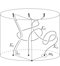
Let be a positive integer. An -component link is a union of simple closed curves in 3-space. In particular, a 1-component link is called a knot. For example, in Figure 1, is a -component link. A link is trivial if it bounds a disjoint union of disks. Two links are equivalent if there is a ‘continuous deformation’ (more precisely, an ambient isotopy) between them.
Let be the unit disk and the diameter on the -axis with same orientation as the -axis. An -string link is a union of simple curves in the cylinder such that the th component runs from to for each , where are points on that are arranged in order along the orientation of . For example, in Figure 2, is a -string link.
Two strings links are equivalent if there is a continuous deformation between them fixing the boundary of . An -string link is trivial if it is equivalent to the -string link .
1.2. Peripheral system and Milnor invariants for links
For an -component link , let be the fundamental group of the complement of . As illustrated in Figure 1, for each component , we choose a pair of elements and in , that are called an th meridian and an th longitude respectively,111While we skip the detailed definition, in this article it is enough to know that meridians and longitudes are special elements in that depend on the link. and we call the pair a peripheral system of . It is known that the peripheral systems up to certain equivalence give the classification of links [23, Theorem 6.1.7]. Hence investigating the equivalence classes of peripheral systems is nothing more than investigating the equivalence classes of links. As we will see below, Milnor invariants are invariants derived from peripheral systems.

Since is non-commutative, classifying peripheral systems is as difficult as classifying links. Therefore we consider the natural projection
where is the commutator subgroup222 is the subgroup generated by the set of . We remark that is a free abelian group generated by . Hence each can be written as
The integer coefficient of is called a (length-2) Milnor invariant of .
More generally, for an integer we consider the natural projection
where for a group , we define and . It is known that is a nilpotent group generated by , and it is called the th nilpotent group of (or the th nilpotent quotient of ). Taking the Magnus expansion , we have an integer with respect to each sequence with length . Here the Magnus expansion is a formal power series in non-commutative variables given by
We denote the integer coefficient of in by . And we define .
The Magnus expansion has the following property.
Proposition 1.1.
For a link , the numbers are determined by a peripheral system . But is not uniquely determined by , and (of length at least 3) are not invariants for . So, for a sequence with length at most , we define
and take the residue class of modulo , which is an invariant for and is called a Milnor -invariant.333A length- Milnor invariant is equal to the linking number between and . Hence Milnor invariants are regarded as a generalization of linking number. V.G. Turaev [35] and R. Porter [36] characterized Milnor invariants by means of Massey product. Moreover, T. Cochran [12] gave a geometric characterization for Milnor invariants as linking numbers of intersections between Seifert surfaces for links, which are closed related to Massey product. K. Murasugi [34] showed that Milnor invariants are given by linking numbers of branched covering space. We note that if the length of is , then , and hence . The length of the sequence is called the length of Milnor invariant . It seems that Milnor invariants depend on , but it is known that Milnor invariants of length at most are equal to those obtained from . Therefore for any sequence with length at most , Milnor invariant is independent of .
As in the case of links, we obtain the integer for a string link . In this case, the meridians and the longitudes are uniquely chosen as illustrated in Figure 2. Hence for all , are invariants for , and they are called Milnor -invariants.
1.3. Automorphisms of nilpotent groups and Milnor invariants
Milnor invariants for string links are defined by N. Habegger and X.S. Lin [20]. Their definition is different from that in the previous section. In this section, we present the idea of the definition by Habegger and Lin.
Set . For an -string link , by Stallings Theorem [41, Theorem 5.1], the inclusion map
induces the isomorphism
for each . Hence we have an isomorphism
Since is the free group generated by the meridians , we have the automorphism
It follows from the definition of that . This means that ‘contains’ the information of Milnor -invariants for . In fact, can be regarded as Milnor invariants of length at most , see Proposition 2.4.
1.4. Properties of Milnor invariants
We summarize the properties of Milnor invariants that are deeply related to the topics in this article.
- (1)
- (2)
-
(3)
(J. Milnor [31], N. Habegger and X.S. Lin [20]) For any sequence consisting of non repeated indices, is link-homotopy invariant [31], where link-homotopy is an equivalence relation generated by changing crossings between strands of the same component. It is known that is link-homotopic to a trivial link if and only if for any non-repeated sequence [31], and that the ’s classify string links up to link-homotopy [20].444This follows from [20, Theorem 1.7], which is not stated in terms of Milnor invariants.
2. Diagrams and Milnor invariants
In this chapter, we define Milnor invariants for welded links, which are defined as a generalization of (diagrams of) classical links, and we also give an algorithm for computing these Milnor invariants.
2.1. Link diagrams
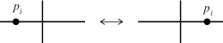
A link is an object in 3-space, but it can actually be ‘drawn’ on the plane, so we may regard it as a figure on the plane. We call this figure a diagram of . In general, a link diagram is a union of closed curves on the plane with finitely many crossings, where each crossing has an ‘over/under information’. Likewise, we can define a string link diagram as a union of curves on the rectangle such that the th component runs from to . A crossing is locally the intersection of two orthogonal line segments, and the point with over (resp. under) information is called over crossing (resp. under crossing), where formally we assume that over and under crossings are distinct points on distinct line segments, see Figure 3.
Two (string) link diagrams are equivalent if one is deformed into the other by a combination of continuous deformations (fixing the boundary) and the three local moves R1, R2, R3 in Figure 4, called Reidemeister moves.
The following theorem shows that the classification of links is nothing more than the classification of link diagrams.
Theorem 2.1.
(Reidemeister Theorem) Two links are equivalent if and only if their diagrams are equivalent.

2.2. Virtual link diagrams and welded links ([22],[19],[16])
While all crossings of link diagrams have over/under informations, we extend the concept of link diagrams by considering diagrams that formally allow crossings without over/under informations as on the left side of Figure 3. A diagram containing crossings without over/under information does not correspond to any link in 3-space. It is an ‘imaginary’ link, so it is called a virtual link diagram. A crossing without over/under information is called a virtual crossing. On the other hand, a crossing with an over/under information is called a classical crossing. For convenience, we also allow the case where there are no virtual crossings in a virtual link diagram. From now on, when we emphasize that link diagrams contain only classical crossings, we call them classical link diagrams.
For virtual link diagrams, we define five local moves as follows. The first four moves in Figure 5 are called virtual Reidemeister moves (VR1,VR2,VR3,VR4), and the last move is called OC move (Overcrossings Commute).
The residue classes of the set of virtual link diagrams modulo continuous deformations, Reidemeister moves, virtual Reidemeister moves and OC moves is called welded links.555The residue classes modulo continuous deformations, Reidemeister moves and virtual Reidemeister moves are called virtual links. Here we never treat virtual links. We define welded string links in a similar way.
The Reidemeister moves, the virtual Reidemeister moves, and the OC move are called the welded moves. As an important property of welded links, the following theorem is known.

Theorem 2.2.
([42],[19]) Two classical link diagrams are equivalent as classical links if and only if they are equivalent as welded links. More precisely, two classical link diagrams are equivalent up to continuous deformations and Reidemeister moves if and only if they are equivalent up to continuous deformations and welded moves.
This theorem implies that there is a natural injection from the equivalence classes of classical links to welded links, i.e., we can say
| ‘classical links can be embedded in welded links.’ |
In this sense, as we mentioned in introduction, the relationship between ‘classical links’ and ‘welded links’ is similar to the relationship between ‘real numbers’ and ‘complex numbers’.
2.3. Based welded links
For an -component virtual link diagram , we choose points on such that each is on the th component of and disjoint from the crossings of . The pair of and is called a based virtual link diagram. Two based virtual link diagrams are equivalent if one is deformed into the other by a combination of continuous deformations, moves as illustrated in Figure 6, and welded moves that do not contain base points. The residue classes of the set of based virtual link diagrams modulo this equivalence relation is called based welded links. Based welded links are ‘between’ welded string links and welded links. In fact we have the following sequence of surjections:
One advantage of considering based welded links is that peripheral systems can be uniquely defined (as explained in the next section). This means that, like string links, based welded links are very ‘suitable’ objects for defining Milnor invariants. In the next section, we define Milnor invariants for based welded links, and by using this definition, we define Milnor invariants for welded string links and for welded links.
2.4. Peripheral systems of based welded links
A diagram of a (based/string) welded link means a representative of the welded link, i.e., a virtual link diagram. However, since it is tedious to distinguish them, the welded link (i.e. the residue class) and its diagram (i.e. a representative) are often identified. From now on we simply call based welded link diagrams based diagrams.
For a based diagram , is divided into several segments by its base points and under-crossings. These segments are called the arcs of . Let be the outgoing arc from the base point , and let be the other arcs of the th component of that appear after in order, when traveling around the th component from along the orientation, where is the number of arcs of the th component (, see Figure 7. Note that is the ingoing arc to
The group of is the quotient group of the free group with generating set modulo the following relations
where denote the arc containing the over crossing between the arcs and as illustrated in Figure 7, and is the sign of the crossing involving and ; in the figure, if the orientation of is from up to down, then , otherwise .
Remark 2.3.
We note that has a group presentation . Let be the group obtained from by adding the relations . We call the group of . It is known that if is a classical link, then is isomorphic to the fundamental group of the complement of .
For each , the two elements and
of are called the th meridian and the th longitude respectively. As in the case of classical links, the pair is called the peripheral system of . We note that the peripheral system of is uniquely determined from the diagram .
2.5. Peripheral systems of diagrams and Milnor invariants
We consider the natural projection
We remark that is a nilpotent group generated by , and it is called the th nilpotent group of (or the th nilpotent quotient of ). Hence each can be written as a word of . Moreover, it is known that for the free group with generating set , we have
see Theorem 2.6. As in the case of string links (see the last paragraph in Section 1.2), by taking the Magnus expansion , we have integers , which are invariants for the based diagram . Since the condition is not essential, we have invariants for all sequences. We call them Milnor -invariants for based welded links.
For a welded string link , by identifying both ends of to a point , we obtain a based diagram . Then we define for all sequences , and call them Milnor -invariants for the welded string link . For a welded link , by choosing a set of base points on , we have a based diagram . And we define Milnor -invariants for the welded link for all sequences as the residue classes of modulo , where
As the names ‘invariants’ suggest, Milnor invariants for welded string links and welded links are invariants under their equivalence relations respectively.
2.6. Automorphisms of nilpotent groups of diagrams and Milnor invariants
For each , since , we have the automorphism
By applying the five lemma to the natural exact sequence
we can see that is an isomorphism. As in the case of classical string links, can be regarded as the Milnor invariants of of length at most . In fact, by using Proposition 1.1, we have the following proposition.
Proposition 2.4.
(cf. [30, Remark 3.6]) Let be a positive integer, and let and be based diagrams. For any sequence of length at most , if and only if , where is the set of automorphisms of that act by conjugation on each generator.
2.7. Colorings of diagrams and Milnor invariants
A map from the set of arcs of a diagram to a group is called an -coloring of if satisfies
for each classical crossing involving and (see Figure 7). Let be a diagram obtained from by a single welded move. Then it is easily seen that there is an -coloring of which coincides with for the arcs not contained in the disk where the welded move is applied.
Let be the normal closure of that contains , and let be the set of arcs of . Then by compositing the natural projection
and , we have the map
Since is an -coloring of and uniquely determined by , is an invariant for . Moreover since , determines the automorphism of the nilpotent group of . By Proposition 2.4, these -colorings can also be regarded as Milnor invariants of length at most .
2.8. Chen-Milnor map and an algorithm for computing Milnor invariants
Here we show how to calculate Milnor invariants of based diagrams. This is simply a rewriting of the method given by Milnor [32] for classical links into one for based diagrams.
Let be a based diagram. For the th component illustrated in Figure 7, we put
(Note that .) Let be the free group generated by . Then, for a positive integer , we define inductively a homomorphism
as follows:777While is essentially the same as defined in [32], in [32] is treated as a single arc.
The map is called Chen-Milnor map [10],[32]. The following lemma can be easily shown by induction on .
Since , by the lemma above, we have the following theorem.
Theorem 2.6.
(J. Milnor [32])
-
(1)
induces an isomorphism
-
(2)
, and hence is a representative of .
Remark 2.7.
Corollary 2.8.
The Milnor invariant for is equal to the coefficient of in the Magnus expansion of , where is an integer with .
Remark 2.9.
As explained above, Milnor invariants are ‘theoretically’ easy to compute. However, when we actually do the calculations, we notice that the length of the word grows exponentially with . Furthermore, performing the Magnus expansion on it, the amount of calculations becomes enormous. Therefore, by this naive algorithm, it is impossible to calculate it even using a computer. Takabatake, Kuboyama and Sakamoto noticed that long words that appear in the process of calculating Milnor invariants contain a lot of repetitions, and by ‘folding’ the words by these repetitions, they succeeded to produce a program that can calculate up to about (depending on the complexity of the links) [43].
Remark 2.10.
Dye and Kauffman’s 2010 paper is often cited as the first paper that tried to extend Milnor invariants to virtual diagrams. However, their paper contains obvious and fatal errors ([24, Remark 4.6], [33, Remark 6.8]). Therefore it should be avoided. In fact, the first successful extension is by Kravchenko and Polyak in [25]. They extended Milnor link-homotopy -invariants to virtual string links. Kotorii then extended Milnor link-homotopy -invariants to virtual links in [24]. Both extensions are invariants of welded diagrams, but restricted to the case of link homotopy invariants. In the general case, Audoux, Bellingeri, Meilhan and Wagner extended Milnor -invariants to welded string links in [1], and Chrisman defined Milnor -invariants for welded links in [11]. In [33], Miyazawa, Wada and the author gave Milnor invariants for (based) welded (string) links using a way completely independent of [1] and [11]. Although these extended Milnor invariants are defined in different ways, they are the same invariant, i.e., for welded (string) links, their values coincide.
3. Characterization of Milnor invariants
In this chapter we discuss the characterization of based diagrams that have the same Milnor invariants. Milnor invariants can be characterized by two equivalence relations, -concordance and self -concordance, on diagrams.
3.1. -concordance and Milnor invariants
The -concordance is an equivalence relation that combines two equivalence relations, -equivalence and welded-concordance, which are explained in the next section. The -equivalence can be seen as a welded version of -equivalence, an equivalence relation on classical links defined by Habiro [21].
B. Colombari [13] showed the following theorem.
Theorem 3.1.
(B. Colombari [13]) Let be a positive integer. Two based diagrams and are -concordant if and only if for any sequence of length at most .
Remark 3.2.
In the paper [13], the statement of Theorem 3.1 is made for welded string links rather than based diagrams. These statements are essentially the same. We can define a product on the set of welded -string links. It is shown that the set of -concordance classes forms a group under the product. Moreover, by using Proposition 2.4 (for the welded string link version) and Theorem 3.1, we can show the following isomorphism
Remark 3.3.
Theorem 3.1 also holds when restricted to classical string links. That is, it completely characterizes Milnor invariants of classical string links. There are many papers that try to characterize Milnor invariants. In particular, the -concordance [28] and Whitney tower concordance [14] are closely related to Milnor invariants, but they cannot give a complete characterization. These studies are done in the ‘real world’ of classical string links and -concordance. On the other hand, Colombari gave the result in the ‘real world’ by expanding his study to the ‘imaginary world’ (i.e., welded string links and -concordance). This is a successful example of how extending the world of classical objects to include welded objects allows us to solve problems from a new perspective.
3.2. -equivalence
The content of this section is due to [29]. Our main purpose here is to introduce the definition of -equivalence. Before explaining -equivalence, some preparation is necessary. From now on, in order to deal with diagrams of (based) welded links and welded string links simultaneously, for convenience, we assume that they are contained in the disk.
3.2.1. -tree
Let be a diagram. A tree that is ‘drawn’ (immersed) on the disk is called a -tree for if it satisfies the following conditions:
-
(1)
The valency of each vertex of is either or , i.e., is a uni-trivalent tree.
-
(2)
The trivalent vertices are disjoint from , and the univalent vertices are contained in and disjoint from the crossings (and base points) of .
-
(3)
All edges are oriented so that each trivalent vertex has two ingoing and one outgoing edge.
-
(4)
We allow only virtual crossings between edges of , and between and edges of .
-
(5)
Each edge of is assigned a number (possibly zero) of decorations, called twists, which are disjoint from all vertices and crossings. (Although base points and twists are both presented by black dots, twists are on edges of and base points are on the diagram .)
A univalent vertex of with outgoing edge is called a tail, and a univalent vertex with an ingoing edge is called a head. From condition (3) above, we can see that a -tree has a unique head, and that specifying the head determines the tails and the orientation of the entire -tree. The tails and head are called ends.
The degree of is the number of the tails of , and a -tree is a -tree with degree . In particular, a -tree is called a -arrow.
For a union of -trees for , vertices are assumed to be pairwise disjoint, and all crossings among edges are assumed to be virtual, see Figure 8 for an example. From now on, when drawing diagrams, we will distinguish them from -trees by drawing them with slightly thicker lines as in Figure 8.

-trees act as ‘guides’ for transforming diagrams locally. Surgery along a -tree is a local move on a diagram using the -tree as a guide, as described below. Before describing surgery along a -tree, we need to explain surgery along -arrow.
3.2.2. Surgery along -arrows
Let be a union of -arrows for . Surgery along yields a new diagram, denoted by , which is defined as follows.
-
(i)
If a -arrow in does not contain any crossing or twist, we perform the operation shown in Figure 9. Note that this operation depends only on the orientation of near the tail of the -arrow.
- (ii)
An arrow presentation for a diagram is a pair of a diagram without classical crossings and a union of -arrows for , such that is equivalent to the diagram . Any diagram admits an arrow presentation since all classical crossings can be replaced with virtual crossings and -arrows as shown in Figure 11.
Two arrow presentations and are equivalent if and are equivalent. An arrow presentation is sometimes treated as a union of a diagram and -arrows , and we do not distinguish them unless necessary. One of the advantages of the arrow presentation is that contains no classical crossings.
3.2.3. Arrow-moves
Arrow moves consist of the virtual Reidemeister moves VR1, VR2, VR3, where they may contain -arrows, and the local moves AR1, …, AR10 in Figure 12. We stress that arrow moves contain no classical crossings. Here the vertical lines in AR1, AR2, AR3 are assumed to be included in diagrams or -arrows, and white dots on -arrows in AR8 and AR10 mean that the -arrows may or may not include twists. Then we have the following.
Theorem 3.4.
Two arrow presentations are equivalent if and only if they are deformed into each other by a combination of continuous deformations and arrow moves, where in the case of based diagram, in addition to VR1, VR2, VR3, the move of Figure 6 is also required, and the local moves AR1, …, AR10 do not include base points.
3.2.4. Surgery along -trees
In the following, we define surgery along W-trees. For an integer , the expansion (E) of a -tree is an operation that replaces a -tree with four -trees of degree less than , as shown in Figure 13. For each figure of Figure 13, the left (resp. right) dashed parts in the figure on the right of ‘’ means the same figures as the left (resp. right) dashed part in the figure on the left of ‘’. The ends of the dashed parts are only the tails of the trees, and their arrangement is chosen arbitrarily. In general, for a -tree , by repeating the expansion we obtain a union of -arrows from (Figure 14). While depends on the arrangement of its tails, thanks to AR7 it is unique up to the arrow moves. Then we define surgery along a -tree as surgery along . In this case, we denote by . Similarly, we define surgery along a union of -trees.
We say that is obtained from by a -move if is a -tree. In particular, we say that is obtained from by a self -move if all ends of are contained in the same component of . Using the move (I) in Figure 15, we can see that is obtained from by a (self) -move, i.e., there is a (self) -tree such that and are equivalent.
Two diagrams and are (self) -equivalent if there is a sequence of diagrams
such that, for each , is equivalent to , or is obtained from by a (self) -move .888It is shown that if , then a (self) -move is realized by (self) -moves [4].
A tree presentation for a diagram is a pair of a diagram without classical crossings and a union of -trees for , such that is equivalent to the diagram . Two tree presentations and are equivalent if and are equivalent. A tree presentation is sometimes treated as a union of a diagram and -trees , and we do not distinguish them unless otherwise necessary.
3.2.5. -tree moves
A local move on a -tree presentation is called a -tree move if it preserves the equivalence classes of the -tree presentations. Here, we introduce four of them given in [29] that will be needed later.
The moves in Figure 15 are called move (I) (Inverse), move (TE) (Tail Exchange), move (HE) (Head Exchange) and move (HTE) (Head Tail Exchange).
In the move (TE), the two tails may be in the same -tree. The right side of the move (HTE) in Figure 15 represents a union of several -trees, each of which has degree greater than the sum of the degrees of the two -trees on the left side. Moves (I) and (TE) are obtained by AR9 and by a combination of AR7 and the expansions of -trees respectively. For the move (HE), by the expansion of the middle -tree of the -tree presentation on the right side and applying the move (I) and AR4, the -tree presentation on the left side is obtained. To obtain the move (HTE), in addition to AR9, AR10, the expansions of -trees and the move (HE), a move called ‘Twist’ (not introduced here) is required. This requires more complex discussions than the other moves, so we omit the details.
3.3. Welded-concordance
Two -component diagrams and are welded-concordant if one can be deformed into the other by a sequence of welded equivalence and the birth/death and saddle moves of Figure 16, such that, for each , the number of birth/death moves is equal to the number of saddle moves, in the deformation from the th component of into the th component of . In the case of based diagrams, the move of Figure 6 is also required, and each local move does not include base points.
It is shown that Milnor invariants for diagrams are welded-concordance invariants [11].

Remark 3.5.
If and are classical links, then the usual link concordance implies the welded-concordance. In the definition of the welded-concordance, the condition on the numbers of birth/death and saddle moves corresponds to the fact that each components of and bounds an annulus in the 4-space. In contrast to the usual link concordance, all welded knots are welded-concordant to the trivial knot [18].
3.4. Ascending presentation and Milnor invariants
In this subsection, we give a sketch of proof of Theorem 3.1 using a special -tree presentation called ascending presentation.
Let be a -tree presentation of a based diagram . Note that is also a based diagram. The -tree presentation is ascending999This notion was first defined in [1], in the context of Gauss diagrams. if, when running around each component of from the base point along the orientation, all tails of appear before all heads of . A based diagram is ascendable if it has an ascending presentation.
3.4.1. Peripheral systems of ascending presentations
Let be an ascendable diagram with an ascending -tree presentation . Since contains no classical crossings, by (after doing expansions of -trees) arrow moves we may assume that is a based diagram , where is a trivial diagram, i.e., it contains no crossings. In the following, we suppose that .
By the expansions of -trees, we obtain a -arrow presentation from the ascending presentation , where for each -arrow in , a small segment adjacent to the head is always assumed to be on the right side with respect to the orientation of the component of that contains the head. Furthermore, we may assume that each -arrow contains at most one twist. We remark that is ascending, since is ascending.
For , we assign a label by arc to the -arrow whose tail is in the -th component of . Let be the free group generated by , let be the labels of -arrows that appear in order, when traveling around the th component of from the base point along the orientation.
Then we define
where if the -arrow corresponding to contains a twist, and otherwise. By the definition of surgery along -arrows, it can be seen that is the sequence of signed labels of the over crossings that appear when running around the th component of from the base point. Moreover, if necessary, by using AR8 move with preserving the ascending presentation, can be regarded as an th longitude . Since is an element of the free group , we have the following proposition.
Proposition 3.6.
([2]) Let and be ascending presentations for ascendable based diagrams and respectively. If for each , then and are deformed into each other by a combination of AR7 and AR9, and hence, and are equivalent.
On the other hand, by Proposition 1.1 (2), we have the following.
Proposition 3.7.
([13]) For any sequence with length at most , if and only if for each , .101010This proposition does not require the assumption of ‘ascending’.
3.4.2. Sketch of the proof of Theorem 3.1
Since the ‘only if’ part of Theorem 3.1 is not difficult to show, we admit that the ‘only if’ part holds and show the ‘if’ part. Also, since the case is obvious, we suppose that .
-
(Step 1)
We deform by -concordance the -tree presentations of and into ascending presentations and , respectively. This can be done by using the move (HTE) and welded-concordance. Doing the expansions of and , we have ascending -arrow presentations and .
- (Step 2)
-
(Step 3)
From an algebraic point of view, we see that is a product of commutators consisting of with length at least . And by applying the inverse of expansion (Figure 17) to the -arrows corresponding to each , we obtain a -tree of degree at least . Hence and are -equivalent.
3.5. Self -concordance and Minor invariants
The content of this section is due to [4]. The self -concordance is an equivalence relation on diagrams obtained by combining self -equivalence and welded-concordance. Here, we introduce the result that the self -concordance classification is given by Milnor invariants.
3.5.1. -reduced quotient groups and Milnor invarints
In this section, we define the -reduced quotient group of a based diagram , and explain the relation between this group and Milnor invariants , where
The arguments in this section are simply rewritings of those in [4] for welded string links into those for based diagrams.
For the peripheral system of , let be the normal closure of that contains . We call the quotient group
the -reduced group of or the -reduced quotient of .
When , it is the link group defined by Milnor [31]. Since is also sometimes called link group, we use a different name here. Habegger and Lin [20] call it the reduced group.
It is known that is a nilpotent group for any positive integer , and
Therefore we have the following surjection.
By composing respectively this with the two maps
defined in Sections 2.5 and 2.7, we have the two maps
Since is generated by , is generated by . Hence is written as a word of .
Let be the free group generated by , and let be the normal closure containing for each . Similar to Theorem 2.6 (1), the following theorem holds.
Theorem 3.8.
The Chen-Milnor map induces the following isomorphism
As in Section 2.7, by the theorem above, is a -coloring.
3.5.2. Self -concordance classification
The following theorem gives the self -concordance classification of based diagrams.
Theorem 3.9.
Let and be based diagrams. Then for any positive integer , the following (1),(2) and (3) are mutually equivalent.
-
(1)
For any sequence with , .
-
(2)
.
-
(3)
and are self -concordant.
Here is the set of automorphisms of that act by conjugation on each generator.
Remark 3.10.
(1) In [4], the statement of Theorem 3.9 is given for welded string links
rather than based diagrams. These statements are essentially the same.
The self -concordant classes coincide with the self -equivalence classes.
The self -equivalence classification of welded string links is given in [1].
(2) The set of self -concordance classes
of welded -string links forms a group under the product of welded string links.
Moreover by using Theorem 3.9 (for the welded string link version),
we can show the following isomorphism
Remark 3.11.
It is shown by T. Fleming and the author [17] that for any sequence with , Milnor invariant is a self -equivalence invariant. The self -equivalence is link-homotopy, and the self -equivalence is often called the self -equivalence. For the case , it is shown in [31] and [45] respectively that a classical link is self -equivalent to a trivial if and only if for any sequence with . The self -concordance classification for classical string links is given in [20] for and in [44] for .
3.5.3. Sketch of the proof of Theorem 3.9
The key for the proof of Theorem 3.9 is ascending presentations, as in the proof of Theorem 3.1. We need two additional theorems below.
A -tree for a diagram is a -tree if at least ends of belong to the same component of . The -equivalence is an equivalence relation on diagrams generated by surgery along -trees, and the -concordance is a combination of the -equivalence and welded-concordance.
Theorem 3.12.
Let be a positive integer. Two diagrams are -equivalent if and only if they are self -equivalent.
Theorem 3.13.
Let and be th longitudes of based diagrams and , respectively. Then for any sequence with if and only if .
Since the proof of is the most difficult, we admit and (and Theorems 3.12 and 3.13) and only give a sketch of proof of .
-
(Step 1)
We deform by -concordance the -tree presentations of and into ascending presentations and , respectively. Doing expansions of and , we have ascending -arrow presentations and . Since a -tree has ends, it is a -tree. Hence, by Theorem 3.12, and are self -equivalent to and respectively.
- (Step 2)
-
(Step 3)
From an algebraic point of view, we have that
-
(a)
if , then is a product of commutators with length at least where appears at least times, and
-
(b)
if , is a product of commutators with length at least where appears at least times.
-
(a)
4. Milnor invariants for surface-links
The content of this and the next chapters is taken from [3]. Milnor invariants can be defined for -dimensional links, which are -manifolds (smoothly embedded) in -space [3]. For simplicity, we explain the case . A 2-dimensional link often means spheres in -space. Milnor invariants introduced here vanish if the fundamental groups of the objects themelves are trivial. Here we consider oriented surfaces, not only spheres, in -space, and call them surface-links. It is possible to consider surfaces with boudary, mimicking string links, but to avoid complications we consider only closed surfaces.
4.1. Surface-link diagrams
As a classical link in -space can be drawn as a diagram in the plane, a surface-link in -space can be drawn as a diagram in -space, for example, see Figure 18. (The arrowed circle in the figure represents the surface orientation. When turning a right hand screw in the direction of , by specifying ‘front’ and ‘back’ of the surface so that the screw moves back to front, the ‘orientation’ of the surface can also be seen as a ‘specifying front/back’.) We note that, in the case of surface-links, the intersections of surfaces appear as curves, and over/under informations are added according to the arrangements in -space by cutting along ‘under-intersections’.

In Figure 18, only ‘simple’ intersections of the surface appear as in the left side of Figure 19. But in general, as in the center of Figure 19, an intersection containing a point called a branch point may appear, and as shown on the right side of Figure 19, three surfaces may intersect, forming a triple point. On the other hand, it is known that by using these three types of intersections, any surface-link can be drawn in 3-space.111111There are two types of branch points, positive and negative, see Figure 23. A diagram drawn in this way is called a diagram of a surface-link.
As there is Reidemeister’s theorem for classical links, there is also the following theorem for surface-links. The local moves on diagrams of surface-links that correspond to Reidemeister moves of classical link diagrams are called Roseman moves.
Theorem 4.1.
In general, by allowing the three kinds of intersections in Figure 19, (-component) surfaces drawn in 3-space are called (-component) surface-link diagrams. When , we often call them surface-knot diagrams. Figure 18 shows a surface-knot diagram. A surface-link diagram is trivial if it has no intersections.
A surface-link diagram can be separated into several regions by under-intersections. For example, the diagram in Figure 18 is separated into 5 regions . For an -component surface-link diagram and for each , we choose a point on a region of the th component. Then we call the pair of and a based surface-link diagram. Two based surface-link diagrams are equivalent if one is deformed into the other by a combination of continuous deformations of 3-space and Roseman moves that do not contain base points.


4.2. Groups of based surface-link diagrams
Let be a based surface-link diagram. We define the group of as follows. For the th component of , let be the region that contains the base point , and let be the other regions, where is the number of regions in . (Unlike classical link diagrams, there are no rules for labeling the regions , and only the region contains the base point .) Let be the free group generated by . For each simple intersection of , we consider a relation as in Figure 20. The group of is the quotient group of the free group with a generating set modulo these relations. It is known that is isomorphic to the fundamental group of the complement of the surface-link whose diagram is .
4.3. Nets of diagrams
In this section, we intuitively explain cut-diagrams of classical links and of surface-links. As we see below, cut-diagrams are ‘nets’ of diagrams.
4.3.1. Cut-diagrams of classical link diagrams
First, we explain cut diagrams of classical link diagrams. The diagram on the left side of Figure 21 is obtained from the circle on the right side by ‘gluing’ points in the arcs to the points \raisebox{-1.1pt}{$A$}⃝, \raisebox{-1.1pt}{$B$}⃝, \raisebox{-1.1pt}{$C$}⃝ respectively so that \raisebox{-1.1pt}{$A$}⃝, \raisebox{-1.1pt}{$B$}⃝, \raisebox{-1.1pt}{$C$}⃝ become under crossings, and the signs of crossings coincide with the signs of the points. From this observation, it can be seen that the circle on the right side of Figure 21 is a net of the diagram on the left side. We call such nets cut-diagrams of link diagrams. That is, a cut diagram of a link diagram is a set of circles with signed points, that correspond to under crossings and are labeled with arcs containing their over crossings.
Remark 4.2.
For the cut-diagram in Figure 21, let be a set of three -arrows such that the tail of belongs to the arc and the head is on the point \raisebox{-1.1pt}{$X$}⃝. And let be an arrow presentation consisting of the trivial knot diagram and , where for each -arrow in , a small segment adjacent to the head is always assumed to be on the right side with respect to the orientation of , and the number of twists is 0 if the sign of the point is positive, or 1 otherwise. Then is an arrow presentation of the knot diagram on the left side of Figure 21. (In general, since may contain more than one -arrows whose tails belong the same arc, is not uniquely determined.) Likewise, from a cut-diagram of any link diagram, we obtain an arrow presentation on a trivial link diagram . For a link diagram , let be an arrow presentation obtained from a cut-diagram of , and let be an arrow presentation of obtained by the operations in Figure 11. Although the heads of and coincide, their tails may not coincide. On the other hand, thanks to AR7 (VR1-VR3 and AR6 if necessary), is equivalent to , and hence it is an arrow presentation of . It follows that two link diagrams that have a common cut-diagram are equivalent as welded links.


4.3.2. Cut-diagrams of surface-link diagrams
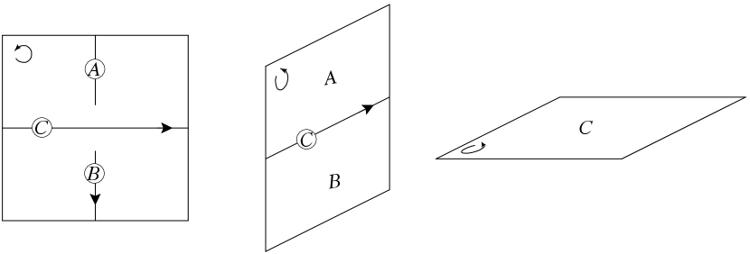
By applying the idea of ‘net’ to surface-link diagrams, we obtain cut-diagrams of surface-link diagrams. The figure on the right side of Figure 22 is a cut-diagram of the surface-link diagram on the left side of Figure 22. In contrast to classical link diagrams, for surface-link diagrams, since the gluing parts are curves, the gluing is specified using oriented, labeled curves on surfaces that correspond to under-intersections.121212These gluing parts without labels are also called lower decker sets [9].
For example, in the cut-diagram on the right side of Figure 22, the curve with label between the regions and intersects the region and is oriented so that, in the gluing result (the left side of Figure 22),
is equal to the right-handed spatial coordinate system


In general, surface-link diagrams may contain branch points and triple points. Then cut-diagrams have ‘local nets’ as illustrated in Figures 23 (resp. 24), which contain end points corresponding to the branch points (resp. classical crossings corresponding to the triple points).

|

|

|

|

|

|

|
|
4.4. Cut-diagrams
In the previous section, we defined cut-diagrams from (surface-)link diagrams. But, in this section, we define cut diagrams independently of (surface-)link diagrams.
4.4.1. -dimensional cut-diagrams
A cut diagram of an -component link diagram can be seen as a set of circles (-dim) with signed points (-dim) arranged on , where each point in is labeled by an arc of . Here, instead of having cut-diagrams from link diagrams, we consider cut-diagrams independently of link diagrams, that are called -dimensional cut-diagrams. That is, an -component 1-dimensional cut-diagram is a triple consisting of a set of circles, a set of signed points on , and a map from a set of arcs of to . For a cut-diagram , we can build a diagram from by gluing it. First, we locally glue only the crossings according to the correspondence of to create classical crossings, and then connect these crossings with corresponding arcs to complete the gluing. If is cut-diagram of a certain link diagram, then we can connect crossings so that the result is equal to the original link diagram. But, in general, when connecting crossings on a plane, new crossings may be necessary. In such cases, a virtual link diagram can be obtained by making the new crossings virtual crossings. Therefore, for any cut-diagram , by gluing it, we have a virtual link diagram . Although might not be uniquely determined, by the observation in Remark 4.2, it is unique up to welded moves. Since we can obtain a cut-diagram from any virtual link-diagram, we have the following sequence of surjections.
While the surjection from cut-diagrams to welded links is not injective, it induces a bijection from a quotient of cut-diagrams modulo certain moves. Here these moves are just the direct translations of welded moves. In this sense, 1-dimensional cut diagrams can be seen as welded link diagrams.
4.4.2. -dimensional cut-diagrams
A cut-diagram of an -component surface-link diagram can be seen as a set of closed surfaces (-dim) with oriented 1-dimensional diagram131313This is almost a link diagram but it may contain end points that correspond to branch points (1-dim), where each arc of is labeled by a region of . Therefore we define -dimensional cut-diagrams independently of surface-link diagrams as a triple consisting of a set of closed surfaces, a -dimensional diagram on , and a map from the set of arcs of to the set of regions of . Here, the map is defined so that ‘local gluing can be performed’ around each branch point and each triple point.141414For a detailed definition, see [3, Subsection 1.2.1]. For an arc of , is called the label of . By putting a circle \raisebox{-1.1pt}{$A$}⃝ on , we mean that the label of is .
Since -dimensional cut-diagrams can be regarded as welded links, -dimensional cut-diagrams can be considered as 2-dimensional generalization of welded links.
4.5. -dimensional cut-diagrams and groups
One important property of cut-diagrams is that they contain gluing information around the intersections. From this information, the group of the original surface-link diagram can be computed from the cut-diagram.
In the following, we define peripheral systems of (based) 2-dimensional cut-diagrams and their Milnor invariants, which induce Milnor invariants for surface-links. From now on, in this chapter, we only treat 2-dimensional cut-diagrams, unless otherwise specified, cut-diagrams always mean -dimensional.
4.5.1. Peripheral systems of based cut-diagrams
For an -component cut-diagram , let be the th component of , and let . For each , let be a point on a region of . Then the pair of and is called a based cut-diagram.
We define the group of as follows. For , let be the region that contains the base point , and let be the other regions, where is the number of regions in . Let be the free group generated by . For each arc of , we consider a relation as in Figure 25. The group of is the quotient group of the free group with generating set modulo these relations. If is a cut-diagram of a based surface-link diagram , then is equal to the group defined in Section 4.2. (Since is independent of the choice of , is called the group of the cut-diagram .)
For an oriented loop on with base point , we define an element in as follows. Let be the sequence of labels of the arcs in that appear in order, when traveling along from following the orientation. While traveling around on the front side of , we define if crosses from left to right, if crosses from right to left. Then we set
where is the sum of signs for .
Lemma 4.3.
If two loops and with base points represent the same element of , then and are equal as elements of .151515By this lemma, the correspondance induces a map . Moreover we have that the map is a homomorphism.
By this lemma, for a loop representing an element , can be seen as an element of . For each , we call the th meridian, and we call
the th longitude set of . The pair is called the peripheral system of .
Let be a set of loops on with base points that represent generators of , and set , where is the minimum number of generators of , i.e., is the genus of . By Lemma 4.3, any element in can be written as a product of elements in . We call an th longitude system.
4.6. Milnor invariants of -dimensional cut-diagrams
In this sction, we define Milnor invariants for cut-diagrams, and also Milnor invariants for surface-links.
Let be the normal closure of that contains the relations of (the group presentation of) , and let . By composing the following sequence
of maps, we have a map
It is known that is a nilpotent group generated by .
In the Magnus expansion of , let be the coefficient of . For sequences and with length at most , we define
and
Then we have the following theorem.
Theorem 4.4.
For any sequences and of length at most , both and are invariants of . In particular they are independent of the choice of .
We define
As for link diagrams, since the condition is not essential, by Theorem 4.4, we have the invariants for all sequences , and call them Milnor invariants of the cut-diagram .
For a surface-link , let be a cut-diagram obtained from a diagram of . For a sequence , we define
Then we have the following theorem.
Theorem 4.5.
If two surface-link diagrams of and are deformed into each other by Roseman moves, then for any sequence .
This theorem implies that of all are invariants of . We call the invariants Milnor invariants of .
4.7. Based cut-diagrams and Chen map
In this section, we explain how to calculate Milnor invariants of 2-dimensional cut-diagrams.
Let be a based cut-diagram. For each region on the th component of , we choose an oriented curve from to a point in .
While running the curve from to , we obtain a word by arranging the labels of arcs, powered by its sign, that appear in order, where the signs are defined in Section 4.5.
Let be the free group generated by . For a positive integer , by using above, we inductively define a homomorphism
as follows.161616The idea of this map was inspired by Chen’s paper [10].
We call the map a Chen map of . The map is different from the case of link diagrams, and it depends on the choices of not only base points but also the curves .
Lemma 2.5 (1) holds for as well. Moreover, the following theorem holds.
Theorem 4.6.
-
(1)
The Chen map induces the following isomorphism.
-
(2)
For any loop with base point , , where is the normal closure of that contains .
By Theorem 4.6 (2), it can be seen that Milnor invariants of are obtained by replacing with in the definition. Hence, gives Milnor invariants of cut-diagrams.
5. Further generalization
For any positive integer , we define -dimensional cut-diagrams, and their equivalence relation, cut-concordance, which corresponds to a generalization of the usual link concordance for -dimensional links.
5.1. -dimensional cut-diagrams and cut-concordance
For a diagram171717See [39], [40], or [37]. of compact -manifold in a compact -manifold , we consider a map
that satisfies ‘certain gluing conditions’.181818For the detailed definition, see [3]. Here ‘regions of ’ correspond to arcs in diagrams in the case of -dimensional cut-diagrams. We call the triple an -dimensional cut-diagram.
Let be a closed -manifold.191919It is not necessary that is closed. But for simplicity we assume that. Two -dimensional cut-diagrams and are cut-concordant if there is an -dimensional cut-diagram that satisfies the following two conditions for each :
-
(1)
There is an orientation preserving diffeomorphism such that .
-
(2)
The following diagram commutes:
Here (resp. ) is a map induced by . The condition (1) implies that and cobound , and the condition (2) implies that the gluing on and can be extended to the gluing on .
The cut-concordance is an equivalence relation on cut-diagrams. This is a generalization of link concordance on -dimensional links, that are embedded -manifolds in the -space. In fact, the following proposition holds.
Proposition 5.1.
If two -dimensional links and are link concordant, then two cut-diagrams obtained from link diagrams of and are cut-concordant.
5.2. Milnor invariants for higher dimensional links.
For an -dimensional cut-diagram , the Milnor invariants can be defined in the same way as for . When , as mentioned in Subsection 4.4.1, the virtual link obtained from is uniquely determined as a welded link. Threfore we define . Then we have the following theorem.
Theorem 5.2.
If two -dimensional cut-diagrams and are cut-concordant, then
for any sequence , the following (1) and (2) hold.
(1) if , (2) if .
Let be a cut-diagram obtained from a diagram of an -dimensional link . For any sequence , we define
Then by Proposition 5.1 and Theorem 5.2 we have the following corollary.
Corollary 5.3.
If two -dimensional links and are link concordant, then
for any sequence , the following (1) and (2) hold.
(1) if , (2) if .
This implies that for an -dimensional link ), is a link concordance invariant of . We call a Milnor invariant of the -dimensional link .
References
- [1] B. Audoux, P. Bellingeri, J.-B. Meilhan and E. Wagner, Homotopy classification of ribbon tubes and welded string links, Ann. Sc. Norm. Super. Pisa Cl. Sci. (5) 17 (2017), no. 2, 713–761.
- [2] B. Audoux and J.B. Meilhan, Characterization of the reduced peripheral system of links, to appear in J. Inst. Math. Jussieu.
- [3] B. Audoux, J.B. Meilhan and A. Yasuhara, Milnor concordance invariants for knotted surfaces and beyond, preprint.
- [4] B. Audoux, J.B. Meilhan and A. Yasuhara, -reduced groups and Milnor invariants, to appear in Math. Research Letters
- [5] H.U. Boden and M. Chrisman, Virtual concordance and the generalized Alexander polynomial, J. Knot Theory Ramifications 30, (2021) Paper No. 2150030, 35 pp.
- [6] A.J. Casson, Link cobordism and Milnor’s invariant, Bull. London Math. Soc. 7 (1975), 39–40.
- [7] J.S. Carter, S. Kamada and M. Saito, Stable equivalence of knots on surfaces and virtual knot cobordisms, J. Knot Theory Ramifications 11(2002), 311–322.
- [8] J. S. Carter and M. Saito, Reidemeister moves for surface isotopies and their interpretation as moves to movies, J. Knot Theory Ramifications 2 (1993), 251–284.
- [9] J. S. Carter and M. Saito, Knotted surfaces and their diagrams, Mathematical Surveys and Monographs, 55 Providence, RI: American Mathematical Society, 1998.
- [10] K.T. Chen, it Commutator calculus and link invariants, Proc. Amer. Math. Soc., 3 (1952), 44—45.
- [11] M. Chrisman, Milnor’s concordance invariants for knots on surfaces, Algebr. Geom. Topol. 22 (2022), 2293–2353.
- [12] T. Cochran, Derivatives of links: Milnor’s concordance invariants and Massey’s products, Mem. Amer. Math. Soc. 84 (1990), no. 427, x+73 pp.
- [13] B. Colombari, A diagrammatic characterization of Milnor invariants, preprint.
- [14] J. Conant, R. Schneiderman and P. Teichner, Whitney tower concordance of classical links, Geom. Topol. 16 2012, 1419–1479.
- [15] R. Fenn, Techniques of geometric topology, London Mathematical Society Lecture Note Series, 57, Cambridge University Press, Cambridge, 1983.
- [16] R. Fenn, R. Rimányi and C. Rourke, The braid-permutation group, Topology 36 (1997), no. 1, 123–135.
- [17] T. Fleming and A. Yasuhara, Milnor’s invariants and self -equivalence, Proc. Amer. Math. Soc. 137 (2009) 761–770.
- [18] R.Gaudreau, Classification of virtual string links up to cobordism, Ars Math. Contemp. 19(2020) 37–49.
- [19] M. Goussarov, M. Polyak and O. Viro, Finite-type invariants of classical and virtual knots, Topology 39 (2000), 1045–1068.
- [20] N. Habegger and X.S. Lin, The classification of links up to link-homotopy, J. Amer. Math. Soc. 3 (1990), 389–419.
- [21] K. Habiro, Claspers and finite type invariants of links, Geom. Topol. 4 (2000), 1–83.
- [22] L. H. Kauffman, Virtual knot theory, European J. Combin. 20 (1999), no. 7, 663–690.
- [23] A. Kawauchi, A survey of Knot Theory, Translated and revised from the 1990 Japanese original by the author. Birkhäuser Verlag, Basel, 1996.
- [24] Y. Kotorii, The Milnor invariants and nanophrases, J. Knot Theory Ramifications 22 (2013), no. 2, 1250142, 28 pp.
- [25] O. Kravchenko and M. Polyak, Diassociative algebras and Milnor’s invariants for tangles, Lett. Math. Phys. 95 (2011), no. 3, 297–316.
- [26] W.Magnus, A. Karrass and D. Solitar, Combinatorial group theory : presentations of groups in terms of generators and relations, Dover books on advanced mathematics, Dover, New York, 1976.
- [27] J.B. Meilhan, Linking number and Milnor invariants Encyclopedia of Knot Theory, Taylor & Francis, (2021), Chapter 83.
- [28] J.B. Meilhan and A. Yasuhara, Characterization of finite type string link invariants of degree , Math. Proc. Cambridge Philos. Soc. 148 (2010) 439–472
- [29] J.B. Meilhan and A. Yasuhara, Arrow calculus for welded and classical links, Algebr. Geom. Topol. 19 (2019), 397–456.
- [30] J.B. Meilhan and A. Yasuhara, Link concordances as surfaces in 4-space and the 4-dimensional Milnor invariants, Indiana Univ. Math. J. 71 (2022), 2647–2669.
- [31] J. Milnor, Link groups, Ann. of Math. (2) 59 (1954), 177—195.
- [32] J. Milnor, Isotopy of links, Algebraic geometry and topology, A symposium in honor of S. Lefschetz, Princeton University Press, Princeton, N. J., (1957), 280–306.
- [33] H.A. Miyazawa, K. Wada and A. Yasuhara, Combinatorial Approach to Milnor Invariants of Welded Links, Michigan Math. J. 73 (2023), 141–170.
- [34] K. Murasugi, Nilpotent coverings of links and Milnor’s invariant, Low dimensional topology, 3rd Topology Semin. Univ. Sussex 1982, Lond. Math. Soc. Lect. Note Ser. 95 (1985), 106–142.
- [35] V.G. Turaev, The Milnor invariants and Massey products, Zap. Nauchn. Sem. LOMI, 66 (1976), 189–203.
- [36] R. Porter, The Milnor’s -invariants and Massey products, Trans. Amer. Math. Soc. 284(1984), 40–424.
- [37] J.H. Przytycki and W. Rosicki, Cocycle invariants of codimension 2 embeddings of manifolds, Knots in Poland III. Proceedings of the 3rd conference, Warsaw, Poland, July 18–25, 2010 and Bȩdlewo, Poland, July 25 – August 4, 2010, (2014) 251–289.
- [38] D. Roseman, Reidemeister-type moves for surfaces in four-dimensional space, Knot theory, Proceedings of the mini-semester, Warsaw, Poland, 1995, (1998), 347–380.
- [39] D. Roseman, Projections of codimension two embeddings, Knots in Hellas ’98. Proceedings of the international conference on knot theory an its ramifications, European Cultural Centre of Delphi, Greece, August 7–15, 1998,World Scientific, (2000) 380–410.
- [40] D. Roseman, Elementary moves for higher dimensional knots, Fundam. Math. bf 184, (2004) 291–310.
- [41] J. Stallings, Homology and central series of groups, J. Algebra, 2 (1965), 170–181.
- [42] T.W. Tucker, Boundary-reducible -manifolds and Waldhausen’s theorem, Michigan Math.J. 20 (1973), 321 – 327.
- [43] Y. Takabatake, T. Kuboyama, H. Sakamoto, stringcmp:Faster calculation for Milnor invariant, available at https://code.google.com/archive/p/stringcmp/
- [44] A. Yasuhara, Classification of string links up to self delta-moves and concordance, Alg. Geom. Topol. 9 (2009), 265–275.
- [45] A. Yasuhara, Self Delta-equivalence for Links Whose Milnor’s Isotopy Invariants Vanish, Trans. Amer. Math. Soc. 361 (2009), 4721–4749.