Microscopic origin of liquid viscosity from unstable localized modes
Abstract
Viscosity is the resistance of a liquid to flow, governed by atomic-scale friction between its constituent atoms. While viscosity can be directly computed using the Green-Kubo formalism, this method does not fully elucidate the physical mechanisms underlying such momentum transport coefficient. In fact, the microscopic origin of liquid viscosity remains poorly understood. In this work, we calculate the viscosity of a metallic liquid and a Kob-Andersen model in a large range of temperatures and compare the results with a theoretical formula based on nonaffine linear response and instantaneous normal mode theory. This analysis reveals that only unstable localized instantaneous normal modes (ULINMs) contribute to viscosity, providing a microscopic definition of viscosity as diffusive momentum transport facilitated by local structural excitations mediated by ULINMs as precursors. Leveraging on the concept of configurational entropy, a quantitative model to connect viscosity with ULINMs is also proposed and validated in both the Arrhenius and non-Arrhenius regimes. In summary, our work provides a microscopic definition of liquid viscosity and highlights the fundamental role of ULINMs as its building blocks, ultimately opening the path to an atomic-scale prediction of viscosity in liquids and glasses.
blueIntroduction\colorblack – Viscosity is a fundamental transport coefficient in fluid dynamics [1] that reflects the ability of transferring momentum in the direction transverse to the motion of the liquid [2]. In the hydrodynamic regime, viscosity governs the flow of physical systems at very different energy scales, from honey [3] to electrons in ultra-clean metallic systems [4] and ultra-relativistic plasma of quarks and gluons [5].
From a macroscopic point of view, shear viscosity is defined by the linear response relation between shear stress and shear strain rate, that can be formalized using Green-Kubo formalism [6, 7]. This method allows for a direct estimate of the viscosity based on the time correlation function of shear stress, but it is limited to Newtonian fluids. Another established method to compute the viscosity is based on the Einstein-Stokes relation between the self-diffusion constant of a probe particle and the mobility of the fluid in which the latter is flowing [8, 9]. However, it is well-known that, as temperature approaches the glass transition, this relation breaks down hindering the applicability of this method.
Moreover, it is important to stress that both the Green-Kubo formula and the Einstein-Stokes relationship do not fully elucidate the microscopic physical mechanisms underlying momentum transport, and ultimately the viscosity itself. In particular, what is the direct link between microscopic dynamics and macroscopic viscosity in a fluid remains an open question. Using a hyperbole, the physical origin of liquid viscosity has not been fully disclosed yet.
In fact, this issue is part of a bigger problem that is the lack of an atomic-scale microscopic description of liquid dynamics and thermodynamics [10, 11], which is mostly due to the absence of a well-defined normal mode formalism for liquids, as achieved on the contrary for crystalline solids [12]. In this context of liquids, the existence of normal modes was already proposed by Zwanzig in 1967 [13], on the basis of Maxwell’s intuition [14] that liquids present solid characteristics at short time scales. These ideas were later formalized by Keyes and collaborators within the so-called instantaneous normal mode (INM) approach [15, 16], that is based on the diagonalization of the Hessian matrix in instantaneous liquid configurations.
Because of the absence of a well-defined equilibrium configuration in liquids, this procedure inevitably leads to the appearance of negative eigenvalues [17], or equivalently purely imaginary frequencies, that correspond to regions of the potential energy landscape with negative local curvature. Modes corresponding to positive eigenvalues are stable, while those with purely imaginary frequencies are called unstable INMs. The physical meaning of these unstable INMs remains matter of debate, contributing to the famous question of “what INMs are and are not” [18].
Partially answering this question, in a series of works [19, 20], Keyes proposed that unstable INMs might provide the fundamental blocks to achieve a microscopic derivation of the liquid self-diffusion constant, highlighting their physical nature as relaxational processes mediated by jumps over potential barriers. It was later clarified that only unstable delocalized INMs contribute to the self-diffusion constant [21, 22] (see also [23, 24, 25, 26, 27, 23, 28] for related works and different definitions of this “diffusive” subset of INMs), providing a first connection between microscopic excitations and macroscopic transport in liquids, but leaving the physical meaning of the localized unstable modes unclear.
In this Letter, we investigate whether a microscopic definition for another fundamental transport coefficient in liquids – shear viscosity– can be achieved using a normal mode approach. In doing so, we will reveal the so-far unknown physical significance of unstable localized modes and their essential role for the microscopic origin of liquid viscosity.
We anticipate that a connection between high-frequency macroscopic elastic moduli and INMs in liquids was already proposed by Stratt [29], alluding to a possible connection between “certain” INMs and liquid viscosity as well. In this Letter, we corroborate that such a relation indeed exists and that unstable localized INMs are the building blocks of liquid viscosity. Our results provide a microscopic definition of viscosity, together with a parameter-free prediction for its value as a function of temperature.
blueTheoretical model and methods\colorblack – According to the theoretical formalism presented in [30] based on nonaffine viscoelastic response [31], the shear viscosity derived from the imaginary part of the complex shear modulus is given by
| (1) |
where represents the number density, is the number of atoms and is the volume of the system. Additionally, is the density of states (DOS); is the atomic mass; is the affine force field correlator [31] (see SM, Appendix D, for more details); is the zero-frequency limit of the spectral density, , with the memory kernel arising from the coupling between tagged particles and thermal environment [32, 33]. All our following results and conclusions will rely on the validity of Eq. (1).
To derive the memory kernel, we use the projection operator formalism [34, 35, 36],
| (2) |
where is the true force acting on the tagged particle. The random force , is the Liouvillian operator corresponding to the unperturbed dynamics and is the Mori projection operator along the direction of the velocity (see SM, Appendix F, for more details). Consequently, the zero-frequency limit of spectral density can be simply expressed as
| (3) |
Finally, we present two important remarks in applying Eq.(1) to liquid systems. First, the definition of the DOS in liquids is not straighforward. In our work, we will identify with the INM density of states, allowing a direct connection to normal modes (that is not possible using the velocity auto-correlation function). Second, following this choice, it is necessary to define the integration range on , that now takes values along both the real and imaginary axes. In the following, in order to find the correct range of integration, we will consider different choices and compare them directly with the simulation data. As already discussed, for the case of the self-diffusion constant [19], only unstable delocalized modes should be considered. It is therefore conceivable that a similar situation will hold for the shear viscosity.
In this study, two simulations systems are considered: (I) a metallic liquid with K [37] and (II) a Kob-Andersen (KA) simulation model [38, 39]. Ten independent samples were obtained to reduce the fluctuation error of the simulations. More details about the models and simulations are provided in the Supplementary Material (SM). The results in the main text refer to the metallic liquid; analogous results for the KA model are presented in the SM and present the same features showing the universality of microscopic origin of viscosity.
We notice that, once the range of integration on in Eq.(1) is fixed, our procedure will not involve any free fitting parameter. Therefore, our results could be taken as a direct test of the validity of Eq.(1) that, to the best of our knowledge, has never been verified.
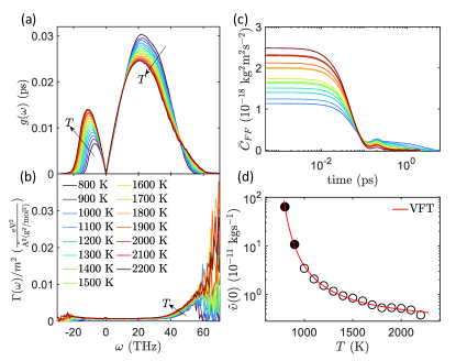
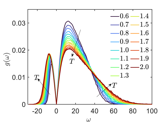
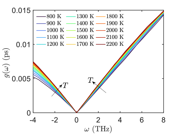
blueMicroscopic description of liquid dynamics\colorblack – We performed INM analysis of the metallic liquid for temperatures between K and K. The corresponding INM DOS is shown in Fig. 1(a), following the common practice of representing imaginary frequencies along the negative axes [15]. The arrows indicate the directions along which increases. We notice that is linear at low frequency (see SM, Fig. S3, for more details), in agreement with theoretical expectations (e.g., [19, 40, 41]) and experimental observations [42, 43].
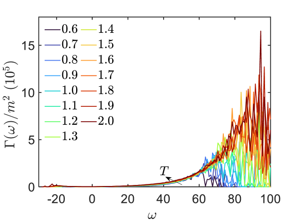
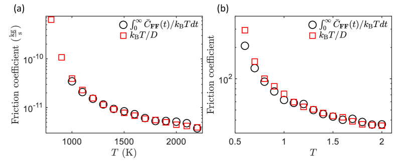
Panels (b) and (c) of Fig. 1 display respectively the re-scaled affine force field versus frequency and the auto-correlation function of the random force versus time at different temperatures. From the memory kernel defined in Eq. (2), we introduce the friction coefficient
| (4) |
Using the Einstein’s relation , where is the long-range diffusion constant of the tagged particles, and comparing Eqs. (3) and (4), we get
| (5) |
We find that computing in this way gives results compatible with those obtained using the projection operator technique, Eq.(3), as shown explicitly in Fig. 1(d). The data also follow the empirical Vogel–Fulcher–Tammann (VFT) equation [44, 45, 46], , shown with a red line in the same panel.
As anticipated, INMs can be classified into stable and unstable modes depending on the sign of the corresponding eigenvalues. The latter can be further divided into localized and delocalized, depending whether the number of particles participating in the mode is intensive or extensive. Bembenek and Laird originally argued that only unstable delocalized modes are related to diffusion [21, 47], while unstable localized modes do not contribute to it. However, there are indications that unstable localized modes may play a fundamental role for other dynamical properties, such as structural relaxation [48, 49].
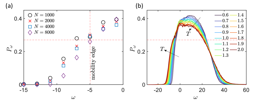
In order to quantify the degree of localization, we consider the participation ratio
| (6) |
where is the contribution of particle to the normalized eigenvector corresponding to eigenfrequency . takes values between and , with the former corresponding to an extremely localized mode with only one particle participating, while the latter to a fully delocalized mode involving all particles (see SM, Fig. S11, for direct visualization of these two types of modes and Ref. [50] for details about ).
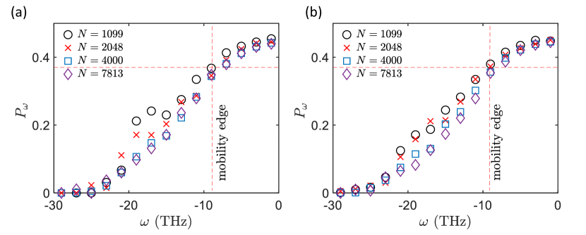
In order to identify the mobility edge separating localized and delocalized modes, we follow [21, 47] and perform a finite size scaling analysis and compute for different . In Fig. 2(a), we show as a function of frequency for the unstable branch of INMs and different system sizes. From there, we can observe that becomes system dependent below a certain threshold frequency, that for the glass-forming system corresponds to . Intensive modes, with below the mobility edge, are localized, while extensive modes with are delocalized.
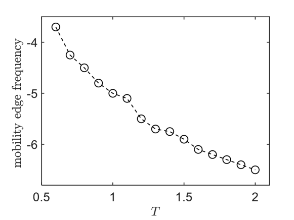
The participation ratio as a function of frequency for different temperatures is shown in Fig. 2(b). By repeating the same finite size scaling analysis for different , we found that the value , defining the mobility edge, is in first approximation independent of temperature (see SM, Fig. S10, for a direct proof of this statement). By then searching for the corresponding (imaginary) frequency (see horizontal dashed line in Fig. 2(b)), we have derived the mobility edge frequency that is plotted in Fig. 2(c) as a function of temperature. We find that the mobility edge frequency increases (in absolute value) by increasing temperature, consistent with the idea that unstable modes tend to be more localized towards the glass transition temperature [21].
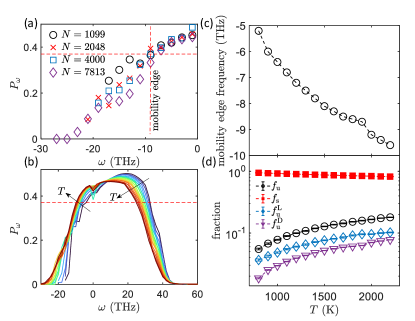
Finally, in Fig. 2(d), we respectively show the fraction of stable , unstable , unstable localized and unstable delocalized INMs in the temperature range considered. We find that the fraction of stable modes slowly decreases by increasing temperature, while all the other fractions increases with temperature following a similar trend. Once the temperature reaches the glass transition, unstable delocalized modes disappear and all unstable modes become localized, consistent with previous results [22].
We have now independently derived all the physical quantities entering in Eq.(1) and analyzed in detail the different types of modes over which the integration therein could be in principle performed. Before moving to the computation of the liquid viscosity, we notice that, due to the limited size of the simulation box , the integration in Eq.(1) will be always performed up to a lower cutoff frequency , where the speed of sound is given by , with the bulk modulus and the mass density (see SM, Appendix H, for more details).
blueLiquid viscosity\colorblack – Traditionally, the viscosity can be computed using the Green-Kubo formula [6, 7],
| (7) |
where is the component of the stress tensor (with ). In Eq.(7), indicates ensemble average. Alternatively, the viscosity can be obtained from non-equilibrium molecular dynamics using the linear response relation , where is the shear strain rate. We will indicate this second route as shear MD.
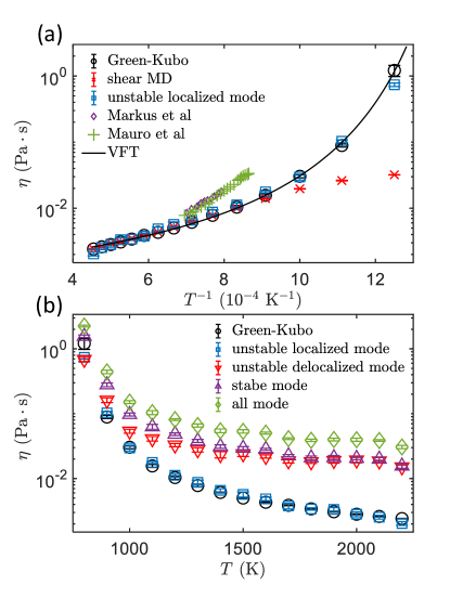
In Fig. 3(a), we compare the viscosity calculated by different methods: black symbols corresponds to the Green-Kubo formula Eq.(7), red crosses to shear MD and blue symbols are the results obtained from Eq.(1), without free parameters, where the integration is performed over only the unstable localized INMs (ULINMs). For comparison, we also show the experimental data from Refs. [51]) (purple diamonds) and [52] (green crosses). At high temperature (above K, times the glass transition temperature), Green-Kubo formula and shear MD are in good agreement. However, when temperature drops, the shear viscosity becomes strain rate dependent and the linear response formula (hence, the shear MD method) is not anymore applicable, giving unreliable predictions for .
Most importantly, we find that the viscosity computed via the Green-Kubo formula is in perfect agreement with the results of Eq.(1) using only ULINMs, and both data are well described by the VFT equation. This is the main result of this work. Same results are obtained for the Kob-Anderson liquid model and are presented in the SM, Fig. S1, confirming the excellent agreement found for the CuZr metallic system and the universality of our conclusions.
For completeness, in Fig. 3(b) we show a comparison between the viscosity obtained from Green-Kubo and the viscosity obtained from the normal mode formula Eq.(1) using different integration regimes or, in other words, different types of INMs as the microscopic building blocks for viscosity. We find that only the estimate using ULINMs is in agreement with the Green-Kubo data. All other choices give results that are almost an order of magnitude away from the correct value of , especially at high temperature. This suggests that unstable localized modes are the microscopic origin of liquid viscosity, and that other excitations are unrelated to this macroscopic transport property.
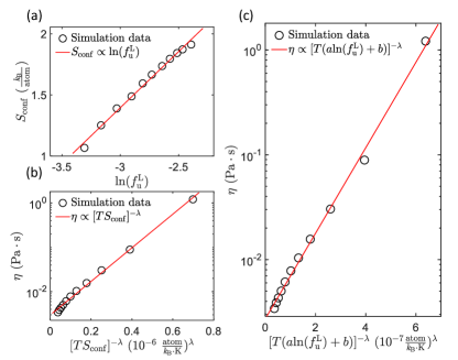
Inspired by Adam-Gibbs theory [53], and motivated by recent results on the relation between liquid diffusion and excess entropy [54], we construct a theoretical model to quantitatively correlate ULINMs with macroscopic viscosity. Following the ideas in [22], we make a similar attempt to link ULINMs to configurational entropy, and then viscosity. First, in Fig. 4(a) we find that the configurational entropy displays a linear relationship with . Here, the configurational entropy is estimated by subtracting the vibrational entropy from the total entropy obtained by thermodynamic integration, as detailed in [55]. Second, we observe that the viscosity follows a direct non-Arrhenius relation with the configurational entropy, , with . We notice the analogy with the connection between the relaxation time and , usually rationalized using random first-order transition theory [53, 56, 57]. By combining these two observations, we conclude that , as demonstrated using the simulation data in Fig. 4(c). This result provides a further link between viscosity and ULINMs and validate their intimate relation, providing a bridge between microscopic and macroscopic physics in liquids.
blueConclusions\colorblack – In this Letter, we have performed MD simulations combined with instantaneous normal mode analysis to disclose the microscopic origin of viscosity in liquids. Our results indicate that unstable localized INMs are the microscopic excitations responsible for this process. Moreover, our work provides a parameter-free formula to predict from normal modes the viscosity of liquids and its temperature dependence, defying the famous Landau argument that is “impossible to derive any general formulae giving a quantitative description of the properties of a liquid” [58].
More in general, our results contribute to answering the question of what unstable INMs are and are not. Unstable delocalized modes are the building blocks for liquid self-diffusion, while the complementary ULINMs are the microscopic facilitators underlying liquid viscosity.
Interestingly, this answer complements several previous analyses. In particular, in Ref.[49] it was shown that localized soft modes are the origin of irreversible structural reorganization. Here, we give a microscopic definition of these localized soft modes and we propose that they should be identified with ULINMs. This is also consistent with the results of [48] that showed that ULINMs act as facilitators of the liquid dynamics, located at the boundary regions between mobile and immobile clusters generated by dynamical heterogeneity. Moreover, our findings are aligned with the idea that, in glass-forming liquid, excitations are localized and relaxation is hierarchical [59]. Finally, viscosity being governed by localized modes is also reflected in the recent results of [60], where it was found that the change in the local barrier energy caused by the fundamental rearrangement or excitation of a few particles (hence, localized modes) determines the change in the activation energy and the dynamics of the supercooled liquids.
In summary, it was repeatedly recognized that “the viscosity of liquids is a subject which has hitherto been without any general theoretical basis” [61]. By identifying the microscopic carriers of momentum transport, our work suggests a possible microscopic and quantitative theory of liquid viscosity, complementing the previous approaches [1] and providing a new path towards a complete understanding of liquid dynamics.
blueAcknowledgments \colorblack – We thank A. Zaccone for collaboration at an early stage of this work and for valuable comments and suggestions. We would like to thank J. Douglas, M. Pica Ciamarra, J. Dyre, T. Keyes, J. Moon and A. Lemaitre for useful comments and discussion. This work was financially supported by the Strategic Priority Research Program (grants nos. XDB0620103 and XDB0510301) and the Youth Innovation Promotion Association of Chinese Academy of Sciences, and the National Natural Science Foundation of China (grant no. 12072344). The numerical calculations in this study were carried out on the ORISE Super-computer. M.B. acknowledges the support of the Shanghai Municipal Science and Technology Major Project (Grant No.2019SHZDZX01) and the sponsorship from the Yangyang Development Fund.
References
- Viswanath et al. [2007] D. S. Viswanath, T. K. Ghosh, D. H. Prasad, N. V. Dutt, and K. Y. Rani, Viscosity of liquids: theory, estimation, experiment, and data (Springer Science & Business Media, 2007).
- Landau and Lifshitz [1987] L. D. Landau and E. M. Lifshitz, Fluid Mechanics (Second Edition) (Pergamon, 1987).
- Garcia et al. [2005] J. M. Garcia, E. Chambers, Z. Matta, and M. Clark, Dysphagia 20, 325 (2005).
- Polini and Geim [2020] M. Polini and A. K. Geim, Phys. Today 73, 28 (2020).
- Shuryak [2004] E. Shuryak, Prog. Part. Nucl. Phys. 53, 273 (2004).
- Green [1954] M. S. Green, J. Chem. Phys. 22, 398 (1954).
- Kubo [1957] R. Kubo, J. Phys. Soc. Jpn. 12, 570 (1957).
- Stokes [2009] G. G. Stokes, Mathematical and Physical Papers, Cambridge Library Collection - Mathematics (Cambridge University Press, 2009).
- Broadbent et al. [1928] T. A. Broadbent, A. B. Einstein, H. Hertz, H. L. Dryden, F. P. Murnaghan, and H. Bateman, The Mathematical Gazette 41, 231 (1928).
- Trachenko [2023] K. Trachenko, Theory of liquids: from excitations to thermodynamics (Cambridge University Press, 2023).
- Moon [2024] J. Moon, Heat Carriers in Liquids: An Introduction (Springer, 2024).
- Moon et al. [2023] J. Moon, L. Lindsay, and T. Egami, Phys. Rev. E 108, 014601 (2023).
- Zwanzig [1967] R. Zwanzig, Phys. Rev. 156, 190 (1967).
- Maxwell [1867] J. C. Maxwell, Phil. Trans. R. Soc. , 49 (1867).
- Keyes [1997] T. Keyes, J. Phys. Chem. 101, 2921 (1997).
- Keyes [2005] T. Keyes, Normal Mode Analysis: Theory and Applications to Biological and Chemical Systems (Chapman and Hall/CRC, 2005) Chap. The Relation Between Unstable Instantaneous Normal Modes and Diffusion.
- Rahman et al. [1976] A. Rahman, M. Mandell, and J. McTague, J. Chem. Phys. 64, 1564 (1976).
- Stratt [1995] R. M. Stratt, Acc. Chem. Res. 28, 201 (1995).
- Keyes [1994] T. Keyes, J. Chem. Phys. 101, 5081 (1994).
- Keyes [1995] T. Keyes, J. Chem. Phys. 103, 9810 (1995).
- Bembenek and Laird [1995] S. D. Bembenek and B. B. Laird, Phys. Rev. Lett. 74, 936 (1995).
- Clapa et al. [2012] V. I. Clapa, T. Kottos, and F. W. Starr, J. Chem. Phys. 136, 144504 (2012).
- Gezelter et al. [1997] J. D. Gezelter, E. Rabani, and B. J. Berne, J. Chem. Phys. 107, 4618 (1997).
- Sciortino and Tartaglia [1997] F. Sciortino and P. Tartaglia, Phys. Rev. Lett. 78, 2385 (1997).
- La Nave et al. [2000] E. La Nave, A. Scala, F. W. Starr, F. Sciortino, and H. E. Stanley, Phys. Rev. Lett. 84, 4605 (2000).
- La Nave et al. [2001] E. La Nave, A. Scala, F. W. Starr, H. E. Stanley, and F. Sciortino, Phys. Rev. E 64, 036102 (2001).
- Chowdhary and Keyes [2002] J. Chowdhary and T. Keyes, Phys. Rev. E 65, 026125 (2002).
- Li and Keyes [1997] W.-X. Li and T. Keyes, J. Chem. Phys. 107, 7275 (1997).
- Stratt [1997] R. Stratt, Int. J. Thermophys 18, 899–907 (1997).
- Zaccone [2023] A. Zaccone, Phys. Rev. E 108, 044101 (2023).
- Lemaître and Maloney [2006] A. Lemaître and C. Maloney, J. Stat. Phys. 123, 415 (2006).
- Cui and Zaccone [2018] B. Cui and A. Zaccone, Phys. Rev. E 97, 060102 (2018).
- Cui et al. [2017] B. Cui, J. Yang, J. Qiao, M. Jiang, L. Dai, Y.-J. Wang, and A. Zaccone, Phys. Rev. B 96, 094203 (2017).
- Carof et al. [2014] A. Carof, R. Vuilleumier, and B. Rotenberg, J. Chem. Phys. 140, 124103 (2014).
- Lesnicki et al. [2016] D. Lesnicki, R. Vuilleumier, A. Carof, and B. Rotenberg, Phys. Rev. Lett. 116, 147804 (2016).
- Jung et al. [2017] G. Jung, M. Hanke, and F. Schmid, J. Chem. Theory Comput. 13 6, 2481 (2017).
- Mendelev et al. [2019] M. I. Mendelev, Y. Sun, F. Zhang, C. Z. Wang, and K. M. Ho, J. Chem. Phys. 151, 214502 (2019).
- Kob and Andersen [1995a] W. Kob and H. C. Andersen, Phys. Rev. E 51, 4626 (1995a).
- Kob and Andersen [1995b] W. Kob and H. C. Andersen, Phys. Rev. E 52, 4134 (1995b).
- Zaccone and Baggioli [2021] A. Zaccone and M. Baggioli, PNAS. 118, e2022303118 (2021).
- Zürcher and Keyes [1997] U. Zürcher and T. Keyes, Phys. Rev. E 55, 6917 (1997).
- Stamper et al. [2022] C. Stamper, D. Cortie, Z. Yue, X. Wang, and D. Yu, J. Phys. Chem. Lett. 13, 3105 (2022).
- Jin et al. [2024] S. Jin, X. Fan, C. Stamper, R. A. Mole, Y. Yu, L. Hong, D. Yu, and M. Baggioli, Scientific Reports 14, 18805 (2024).
- Vogel [1921] H. Vogel, Phys. Z 22, 645 (1921).
- Fulcher [1925] G. S. Fulcher, J. Am. Ceram. Soc. 8, 339 (1925).
- Tammann and Hesse [1926] G. Tammann and W. Hesse, Z. Anorg. Allg. Chem 156, 245 (1926).
- Bembenek and Laird [1996] S. D. Bembenek and B. B. Laird, J. Chem. Phys. 104, 5199 (1996).
- Zhang et al. [2019] W. Zhang, J. F. Douglas, and F. W. Starr, J. Chem. Phys. 151, 184904 (2019).
- Widmer-Cooper et al. [2008] A. Widmer-Cooper, H. Perry, P. Harrowell, and D. R. Reichman, Nat. Phys. 4, 711 (2008).
- Mizuno and Ikeda [2023] H. Mizuno and A. Ikeda, in Low-Temperature Thermal and Vibrational Properties of Disordered Solids: A Half-Century of Universal “Anomalies” of Glasses (World Scientific, 2023) pp. 375–433.
- Mohr et al. [2019] M. Mohr, R. K. Wunderlich, S. Koch, P. K. Galenko, A. K. Gangopadhyay, K. F. Kelton, J.-Z. Jiang, and H.-J. Fecht, Microgravity. Sci. Tec. 31, 177 (2019).
- Mauro et al. [2014] N. Mauro, M. Blodgett, M. Johnson, A. Vogt, and K. Kelton, Nat. Commun. 5, 4616 (2014).
- Adam and Gibbs [1965] G. Adam and J. H. Gibbs, J. Chem. Phys. 43, 139 (1965).
- Douglass et al. [2024] I. M. Douglass, J. C. Dyre, and L. Costigliola, Phys. Rev. Lett. 133, 068001 (2024).
- Cao and Wang [2024] L.-L. Cao and Y.-J. Wang, J. Phys. Chem. Lett. 15, 811 (2024).
- Bouchaud and Biroli [2004] J.-P. Bouchaud and G. Biroli, J. Chem. Phys. 121, 7347 (2004).
- Ozawa et al. [2019] M. Ozawa, C. Scalliet, A. Ninarello, and L. Berthier, J. Chem. Phys. 151 (2019).
- Landau and Lifshitz [1980] L. D. Landau and E. M. Lifshitz, Statistical Physics: Volume 5, Vol. 5 (Pergamon, 1980).
- Keys et al. [2011] A. S. Keys, L. O. Hedges, J. P. Garrahan, S. C. Glotzer, and D. Chandler, Phys. Rev. X 1, 021013 (2011).
- Ciamarra et al. [2024] M. P. Ciamarra, W. Ji, and M. Wyart, PNAS. 121, e2400611121 (2024).
- Andrade [1930] E. d. C. Andrade, Nature 125, 309 (1930).
- Nosé [1984] S. Nosé, J. Chem. Phys. 81, 511 (1984).
- [63] https://www.lammps.org/ .
- Hill [1952] R. Hill, Proc. Phys. Soc. A 65, 349 (1952).
- Gottwald et al. [2015] F. Gottwald, S. Karsten, S. D. Ivanov, and O. Kühn, J. Chem. Phys. 142, 244110 (2015).
Supplementary Material
Microscopic origin of liquid viscosity from unstable localized modes
Long-Zhou Huang, Bingyu Cui, Vinay Vaibhav,
Matteo Baggioli, Yun-Jiang Wang
In this Supplementary Material (SM), we provide further details about the numerical and analytical computations presented in the main text. Moreover, we show further analysis on a Kob-Andersen model to corroborate our findings.
Appendix A Metallic liquid
A semi-empirical potential function is used to simulate the interactions in a metallic glass with a simulation box of 4000 atoms [37]. The liquid and glass samples are prepared with the standard heating-cooling method. First, a crystalline phase was heated from 300 K to 2300 K for melting. And then the liquid is thermally equilibrated for 1 ns at 2300 K which is much longer than the relaxation time. Then the equilibrium liquid was quenched to supercooled liquid to 300 K with constant cooling rate of K/s. The above sample preparation process was carried out under the NPT ensemble with periodic boundary condition. The Nose-Hoover thermostat was used to control temperature and the barostat was used to keep pressure to zero [62]. The kinetic properties were estimated using standard microcanonical (NVE) ensemble after sufficient equilibration at each specific temperature. For statistical purpose, ten independent samples were simulated to reduce the fluctuation of physical quantities. The velocity Verlet algorithm was used to integrate Newton’s equations of motion with a time step of 1 fs.
Appendix B Kob-Andersen model
The Kob-Andersen model is binary Lennard-Jones mixture introduced by Kob and Andersen [38, 39] and defined by the following LJ potential,
| (S1) |
where ; here , and . The KA model consists of particles A and B with the same mass in a ratio of 80:20. We use reduced units, where length is in the unit of , temperature , and time . Under periodic boundary conditions, the system contains 4000 particles. Under the NVT ensemble, the fixed density is 1.185 and the cooling rate is . The kinetic properties were calculated using standard microcanonical (NVE) ensemble. Ten independent samples were obtained to reduce the fluctuation error of the simulations. The time step is 0.005. For the KA model, the temperature will be always displayed in reduced LJ units.
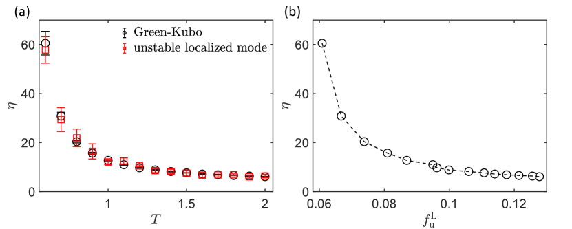
As it can be seen from the Fig. S1(a), the relationship between viscosity and unstable localized mode of Kob-Anderson model is similar to that found in metallic system, which justifies that the generality of our observation that unstable localized mode are is the physical origin of viscosity in liquid. As shown in Fig. S1(b), the viscosity decreases by increasing the fraction of unstable localized modes. This is consistent with the fact that grows with temperature and the viscosity decreases while increasing temperature in the liquid phase.
Appendix C Instantaneous normal modes
The dynamical matrix for the instantaneous liquid configuration at a given temperature (instantaneous Hessian matrix) is given by
| (S2) |
where is the mass of particle and is the coordinate ( or ) of particle . We directly diagonalize the dynamical matrix and calculate the vibrational density of states as
| (S3) |
where is the eigenfrequency. Ten independent samples were obtained to reduce the fluctuation error of the simulations.
The results for the INM DOS are shown in Fig. S2 and present similar features as for the metallic liquid discussed in the main text.
A zoom of the low frequency region of for the metallic glass-forming liquid is shown in Fig. S3. The data confirm the linear scaling (with growing with temperature) discussed in the main text.
Appendix D Affine force field correlator
According to nonaffine lattice dynamics theory [31], the affine force field is obtained from
| (S4) |
where is the force on the atom in deformed state; is the force on the atom in undeformed state; is the simple shear strain. The projection of the eigenvectors of the Hessian matrix onto the affine force field are then given by
| (S5) |
and the affine force field correlator is derived from
| (S6) |
A shear strain of 0.0001 is applied in our simulation of Kob-Anderson model and metallic glass. The affine force field correlator of the Kob-Anderson model is shown as a function of frequency, for the liquid sample at different temperature as shown in the Fig. S4.
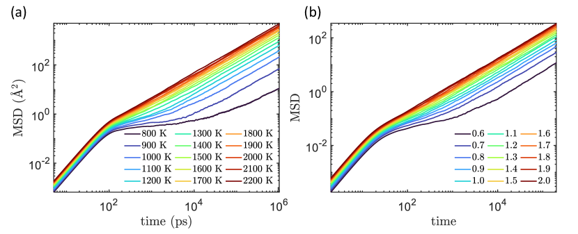
Appendix E Mean square displacement
The diffusion constant can be obtained from the mean square displacement (MSD) as a function of time
| (S7) |
The average diffusion constant in an isotropic system in 3D is given by
| (S8) |
Appendix F Projection operator technique
According to the projection operator technique [34, 35, 36], the memory kernel
| (S9) |
where the true force acting on the tagged particle. Based on the second-order backward algorithm, , where is an observable, and . evolves according to the backward orthogonal dynamics
| (S10) |
where and are respectively the atomic positions and momenta. The second-order propagator
| (S11) |
with
| (S12) |
| (S13) |
| (S14) |
| (S15) |
As a result, based on the trajectories of the atoms in each configuration we can get . Finally, can be obtained,
| (S16) |
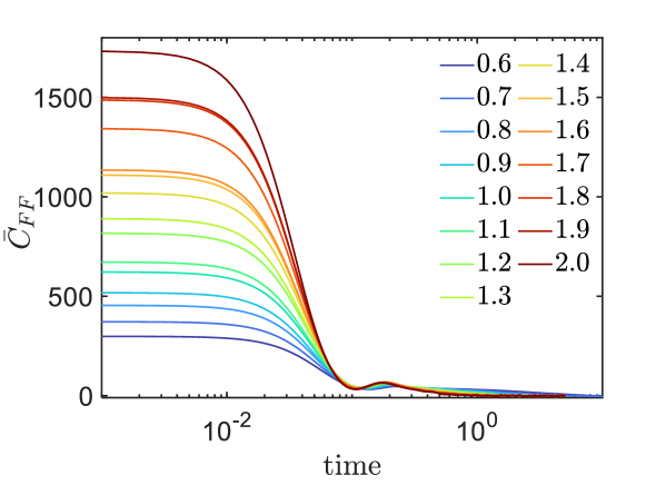
As shown explicitly in Fig. S7, the results for the friction coefficient obtained using and are in good agreement. Therefore, we will use , instead of , to calculate at low temperatures.
Appendix G Participation ratio
The participation ratio of Kob-Anderson model is calculated and analyzed in Fig. S8 and displays features similar to the case of the metallic glass-forming liquid discussed in the main text.
As done in the main text, we can calculate the dependence of the mobility edge frequency on temperature for the KA model, as shown in the Fig. S9.
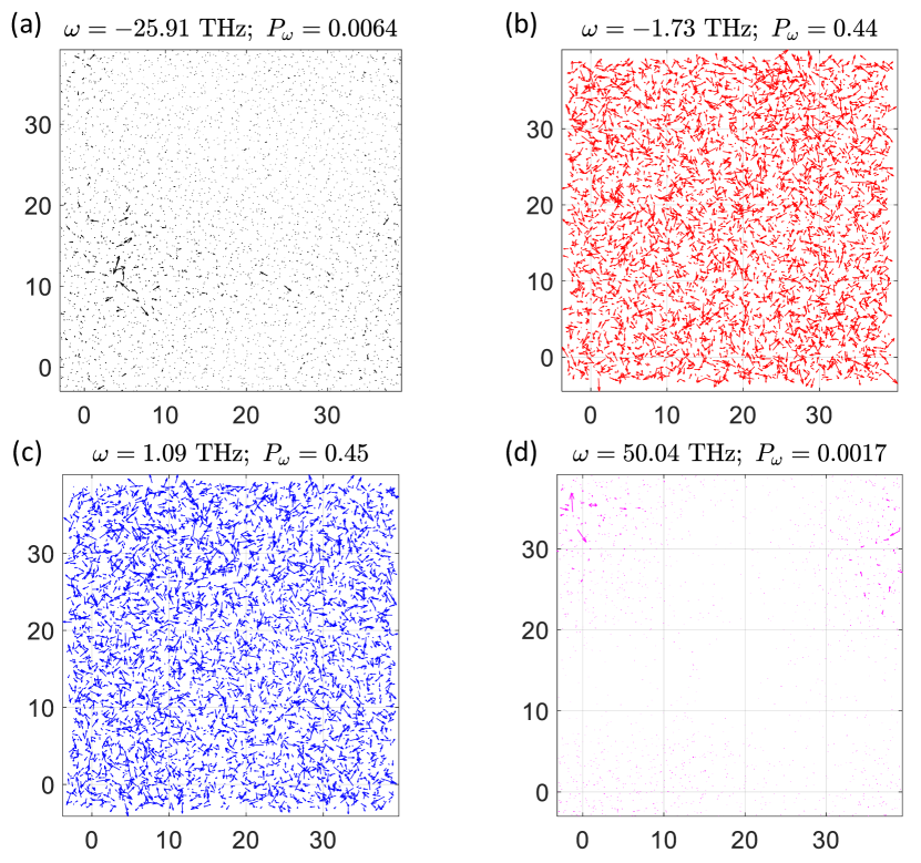
Meanwhile, variation of the participation ratio of metallic glass-forming liquid as a function of (imaginary frequency) at K and K upon changing the size of the simulation box as shown in the Fig. S10. A typical localized and delocalized mode are shown by the magnitude of each particles vibrational vector as shown in the Fig. S11. Several high amplitude eigenvectors at local frequencies indicate strong localization, indicating that the energy associated with these modes is confined to a small spatial region.
Appendix H Bulk modulus
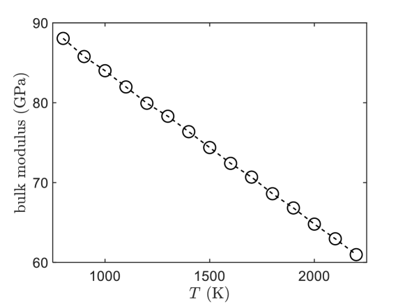
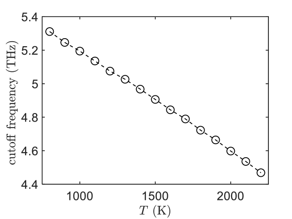
The elastic constants are calculated using LAMMPS [63], and then bulk modulus can be obtained according to the Voigt-Reuss-Hill approximation [64]. In the Fig. S12, it is shown that the bulk modulus of decreases with increasing temperature. Fig. S13 shows the value of the cutoff frequency, , as a function of temperature for the metallic liquid.
Appendix I Vogel-Fulcher-Tammann (VFT) equation
Appendix J Generalized Langevin equation (GLE)
The linear generalized Langevin equation (GLE) is given by [65]
| (S18) |
where is the frequency of an effective harmonic oscillator. Multiplying the linear GLE with and taking a canonical ensemble average, we can get
| (S19) |
By using the relation
| (S20) |
Eq. S19 can be simplified in the following form
| (S21) |
where
| (S22) |
Upon Fourier transforming Eqs. (S21) and (S22), one obtains
| (S23) |
| (S24) |
Comparing Eqs. (S23) and (S24), we finally obtain
| (S25) |