Metastability associated with many-body explosion of eigenmode expansion coefficients
Abstract
Metastable states in stochastic systems are often characterized by the presence of small eigenvalues in the generator of the stochastic dynamics. We here show that metastability in many-body systems is not necessarily associated with small eigenvalues. Instead, many-body explosion of eigenmode expansion coefficients characterizes slow relaxation, which is demonstrated for two models, interacting particles in a double-well potential and the Fredrickson-Andersen model, the latter of which is a prototypical example of kinetically constrained models studied in glass and jamming transitions. Our results provide insights into slow relaxation and metastability in many-body stochastic systems.
I Introduction
Metastability in stochastic systems is ubiquitous in nature. In particular, it is often associated with first-order phase transitions Langer (1969, 1974); Penrose (1995), (spin) glasses Bray and Moore (1980); Biroli and Kurchan (2001); Berthier and Biroli (2011), protein folding Baldwin et al. (2011), and so forth. Despite its importance, the definition of metastability is quite subtle. In mean-field models, there is a static characterization of metastable states, i.e., local minima of the free energy as a function of order parameters Griffiths et al. (1966). For non mean-field models, however, a metastable state has a finite lifetime even in the thermodynamic limit Lanford and Ruelle (1969), and hence we should treat metastability as a timescale-dependent dynamical concept 111See Refs. Langer (1969); Penrose (1995) for attempts to give a static characterization of finite-lifetime metastable states associated with first-order phase transitions via an analytic continuation of the thermodynamic function..
Since the generator of the master equation contains full information on the stochastic dynamics, it is natural to expect that metastability is dynamically characterized by some special properties of eigenvalues and/or eigenvectors of . Indeed, the real part of an eigenvalue of gives the decay rate of the corresponding eigenmode, which suggests that metastability is characterized by the presence of small eigenvalues separated from the other large eigenvalues Gaveau and Schulman (1998); Bovier et al. (2000); Biroli and Kurchan (2001) (see Refs. Macieszczak et al. (2016); Rose et al. (2016, ) for quantum systems). Such a spectral characterization of metastable states is appealing since it is purely dynamical; we do not have to rely on thermodynamic notions such as the (free) energy landscape, which is difficult to define precisely except for mean-field models Frenkel (2013).
In this paper, we revisit this problem. We show that metastability in many-body stochastic systems does not necessarily accompany small eigenvalues. By analyzing two simple models, i.e. interacting particles in a double-well potential and the Fredrickson-Andersen (FA) model Fredrickson and Andersen (1984), we demonstrate that slow relaxation in those models is characterized by many-body explosion of eigenmode expansion coefficients, which was recently studied in the context of open quantum systems Mori and Shirai (2020); Haga et al. (2021) (see also Ref. Bensa and Znidaric ). Our results provide insights into slow relaxation and metastability in many-body stochastic systems.
The remaining part of the paper is organized as follows. In Sec. II, we give a general formulation within a framework of classical Markov processes on discrete states. We introduce eigenmode relaxation times in Sec. II.2. In Sec. III, we numerically show that eigenmode expansion coefficients become huge for concrete models. In Sec. III.1, we consider non-interacting particles in a double-well potential. Metastability in this model is due to large barrier of a single-particle potential, and hence we call it “potential-induced metastability”. In Sec. III.2, we consider the same model with inter-particle interactions. Metastability is induced by strong inter-particle interactions, and hence we call it “interaction-induced metastability”. In Sec. III.3, the FA model is investigated. Metastability in this model is due to kinetic constraints and not of energetic origin. It turns out that potential-induced metastability can be explained by the emergence of vanishingly small eigenvalues, whereas the other two are not associated with small eigenvalues: they are explained by many-body explosion of expansion coefficients. Finally, we discuss our results in Sec. IV.
II General formulation
II.1 Setup
Let us consider a system with discrete states . The energy of the state is denoted by . The probability distribution evolves following the master equation
| (1) |
where the matrix is the generator of the stochastic dynamics. For , represents the transition rate from the state to , and . When the system is coupled to a thermal bath at the inverse temperature , satisfies the detailed-balance condition, .
The detailed-balance condition ensures that is diagonalizable with real (and non-negative) eigenvalues since it is made symmetric via the similarity transformation with . We here assume that the stationary state is unique and eigenvalues are ordered as . The right and left eigenvectors for an eigenvalue are respectively denoted by and : and .
Let us normalize right eigenvectors by using the norm as follows:
| (2) |
where are th component of . We will later see that this normalization is convenient for our purpose. Since the dual norm of the norm is the norm in the sense that for any set of vectors and , we normalize left eigenvectors by using norm as follows:
| (3) |
where are th component of .
The mode corresponds to the stationary state, and with and for all . Without loss of generality, we choose the signs of and so that and .
The probability distribution can be expanded in terms of right eigenvectors of as , where
| (4) |
is an eigenmode expansion coefficient in the initial state.
II.2 Eigenmode relaxation time
Obviously, gives the decay rate of th eigenmode, and hence the slowest decay rate is given by the spectral gap of . This observation indicates that slow relaxation should accompany small . Following this idea, in previous works Gaveau and Schulman (1987, 1998); Biroli and Kurchan (2001); Macieszczak et al. (2016), metastability is characterized by the presence of small eigenvalues. This argument implicitly assumes that is not too large. As we point out below, however, this assumption is typically not satisfied in many-body systems.
For a given initial state , let us define the relaxation time for each eigenmode. The expectation value of a physical quantity with is given by
| (5) |
The contribution from th eigenmode is thus bounded as
| (6) |
where the normalization (2) is used. Thus the contribution from th eigenmode is negligible when , and hence it is appropriate to define the eigenmode relaxation time as the time at which for a fixed constant . Throughout the paper, we fix .
We then have
| (7) |
which implies that large expansion coefficients can cause the delay of the relaxation 222If we choose another normalization condition for right eigenvectors, the criterion of the relaxation should be modified. For example, if we employ the normalization , we have , and hence the criterion of the relaxation should be with being a fixed constant. Accordingly, the formula (7) should also be modified. In other words, Eq. (7) is appropriate only for the normalization scheme (2).
Which eigenmodes are responsible for metastable states? To answer this question, let us examine the possible largest value of over all initial distributions. From Eq. (4), we have an upper bound
| (8) |
This upper bound is always realizable: when is nonzero only for such that . Thus, we obtain
| (9) |
The eigenmode relaxation times tell us about which eigenmodes can compose metastable states. In bra-ket notation, the time evolution operator is written as
| (10) |
For a timescale specified by , we consider a subset of eigenmodes such that for any . Since for , we have , which implies that a metastable state consists of eigenmodes in .

III Metastability and explosive growth of eigenmode expansion coefficients
In this section, we show that becomes huge and significantly changes the relaxation time in many-body stochastic models, i.e., an -particle system in a double-well potential and the FA model. Through the analysis of those models, we consider three kinds of metastability, i.e., the potential-induced metastability, the interaction-induced metastability, and the metastability due to kinetic constraints. It is shown that the potential-induced metastability is associated with small eigenvalues, whereas the others are caused by an explosive growth of expansion coefficients .
III.1 Non-interacting particles in a double-well potential
Let us begin with the simplest model, i.e., independent particles in a double-well potential under the two-state approximation (see Fig. 1). Each particle () is either in the left or right well, which is expressed by a spin variable ( corresponds to the left well). Then -particle state is specified by a set of spin variables , and there are different states. The state (left well) has the energy , and the energy barrier undergoing in the transition from to is given by . By choosing the temperature as the unit of energy (i.e., ), transitions of th particle from to and vice versa happen at rates given by the Arrhenius law and , respectively. Here, is a certain microscopic timescale, which is chosen as the unit of time, i.e., . This transition rate satisfies the detailed-balance condition for the Hamiltonian , where the number of particles in the left well is denoted by . Similarly, we define as that in the right well.
In the single-particle problem, the generator is a two-by-two matrix, and it has two eigenvalues and . The right and left eigenvectors are denoted by and ( or 1), respectively. In the -particle case, the eigenvalues are given by the sum of single-particle eigenvalues as , where specifies which eigenmode is occupied by th particle. The corresponding eigenvectors are given by the product of single-particle eigenvectors: and .
The maximum expansion coefficient in Eq. (8) for each is explicitly calculated as follows:
| (11) |
When , for . Expansion coefficients diverge exponentially in . Although the corresponding eigenvalue is extensively large , it is not correct that this eigenmode decays in a timescale . The eigenmode relaxation time is evaluated as
| (12) |
whose second term is independent of the system size and .
In this model, the “all-left” state, i.e., , is considered to be a many-body metastable state for large . Expansion coefficients for this state are explicitly calculated, and it is found that and for all , i.e., this state gives the maximum expansion coefficients for all eigenmodes.
Even in this simplest case, explosive growth of expansion coefficients occurs. However, does not depend on , and hence large is not related to metastability in this non-interacting model.
III.2 Interacting particles in a double-well potential
Let us introduce interactions. We here consider a simple model in which two particles in the same potential well equally interact with each other. The interaction energy is given by , where denotes the interaction strength (the scaling ensures the extensivity of the energy). The interaction changes the effective potential felt by a single particle: the energy is written as with and . The effective energy barrier from to is thus given by . The model with interactions is obtained by replacing in the non-interacting model by . Obviously, interactions effectively increases the energy barrier and causes slower relaxation, which we call interaction-induced metastability.
The master equation in this model is generated by a -dimensional generator. Instead of considering the full generator, let us employ the simplified description by focusing on the dynamics of a collective variable only. Since the energy only depends on in our model, we can exactly obtain the dynamics of . Let the probability distribution of at time be denoted by . Then the master equation for is written as
| (13) |
where . This generator satisfies the detailed-balance condition of the form
| (14) |
where denotes the free energy of a state specified by . The entropy is given by .
The -dimensional generator in Eq. (13) is a diagonal block of the original -dimensional full generator. Thus, the full generator has other eigenmodes, which are dropped in this description. However, it does not affect the conclusion (see Appendix A).
We now fix and . In our model, there is the non-ergodic phase for , in which we have an extensive free energy barrier and the relaxation time diverges in the thermodynamic limit as . We discuss the non-ergodic phase in Appendix B, and here we focus on the ergodic phase at which the free energy is a monotonic function of .
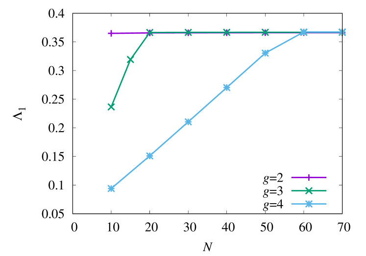
First let us investigate the -dependence of the spectral gap of . Numerical results for different and are presented in Fig. 2. It clearly shows that the spectral gap of is almost independent of the value of for large , although the finite-size effect is stronger for larger . It means that the spectrum gap does not reflect the increase of the relaxation time due to interactions.
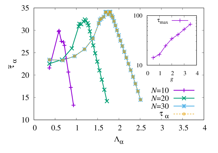
Next, we compute at for different and show the result in Fig. 3. Although the typical value of linearly grows with , that of looks convergent for large . According to Eq. (9), it means that expansion coefficients typically grows exponentially in , which is already seen in the non-interacting model. In Fig. 3, for the all-left initial state is also plotted by squares with a dashed line in Fig. 3, which completely agrees with as in non-interacting case. The all-left state has the maximum expansion coefficients for all eigenmodes, .
It turns out that the eigenmode that gives the largest relaxation time appears in the middle of the spectrum, , not at the spectrum edge. Since the relaxation particularly slows down far from equilibrium with large , an extensive number of particles simultaneously undergo dissipation in a many-body metastable state, which would be the reason why eigenmodes with extensively large eigenvalues are important here.
We plot against in the inset of Fig. 3. We find that increases exponentially in , which is consistent with the intuitive picture that interactions effectively increase the energy barrier. This increase of the relaxation time stems from rapid growth of expansion coefficients with .
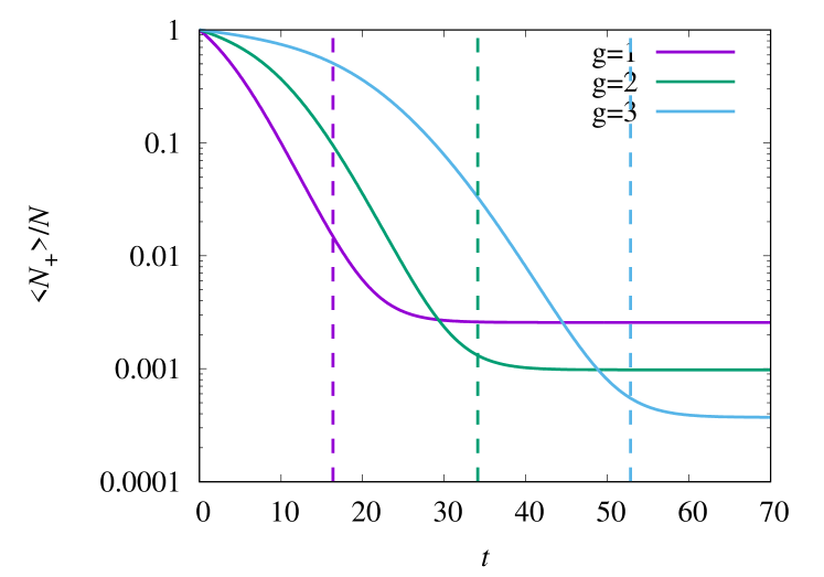
In order to compare the physical relaxation time with , we numerically compute the dynamics of starting from the all-left initial state. The numerical result for different at is shown in Fig. 4. The quantity reaches the stationary value roughly at , which is shown by vertical dashed lines in Fig. 4. It is thus confirmed that coincides with the physical relaxation time of the system.
III.3 Fredrickson-Andersen model
In the model considered so far, interaction-induced metastability is explained by the many-body explosion of expansion coefficients. Here we examine the FA model Fredrickson and Andersen (1984) as a prototypical example of kinetically constrained models Ritort and Sollich (2003) studied in glass and jamming transitions Berthier and Biroli (2011). Metastability in a kinetically constrained model is not due to energy barriers but due to dynamical rules. As we see below, the many-body explosion of expansion coefficients also explains this kind of metastability.
Suppose that each site is occupied () or empty (), and the transition rates from to 1 and that from to 0 are given by and , respectively, where corresponds to the average density at equilibrium and expresses dynamical constraints. In the FA model Fredrickson and Andersen (1984), , which means that the site can change its state only if at least one of the two neighbors and is empty. Since this transition rate satisfies the detailed balance condition with respect to the non-interacting Hamiltonian , where denotes the chemical potential, the equilibrium state is trivial but its dynamics exhibits interesting properties, which is a common characteristic of kinetically constrained models.
In the FA model, it is rigorously proved that the spectral gap of remains finite in the thermodynamic limit for any Cancrini et al. (2008). However, the maximum relaxation time exhibited by this model diverges in the thermodynamic limit for any . Because of the kinetic constraint, a cluster of particles can decay or grow only from its edges. Therefore, if the initial state has a macroscopically large cluster of size , the relaxation time is at least of . A state with macroscopically large clusters is therefore regarded as a metastable state. This increase of the maximum relaxation time should be due to an exponential growth of 333At , the Hamiltonian vanishes and is a symmetric matrix. Even in this case, the many-body explosion of expansion coefficients occurs..
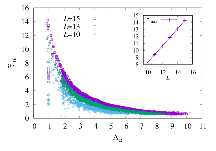
Under the periodic boundary condition, for are computed and plotted in Fig. 5. We see that in the FA model for with , which results in even though the spectral gap remains finite.
IV Discussion
We have shown that the many-body explosion of eigenmode expansion coefficients is responsible for slow relaxation in many-body stochastic systems. We emphasize that this is a generic phenomenon, and it would also occur in nonequilibrium dynamics without detailed balance. Concepts related to slow relaxation, such as metastable states, must be reconsidered.
Since the maximum value of the expansion coefficient for an eigenmode is given by the inverse of the overlap between the left eigenvector and the right eigenvector , the many-body explosion of indicates a mismatch between the supports of these two vectors. Under the detailed balance condition, left and right eigenvectors are given by and , where is the eigenvector of the symmetric matrix with the eigenvalue . Therefore, the support of () tends to be localized at low (high) energies, which may result in an extremely small overlap . We however point out that explosive growth of occurs even when is a symmetric matrix, i.e., , which is realized in the FA model with . We also emphasize that it would also occur in nonequilibrium stochastic dynamics without detailed balance.
In the two models examined in this work, are broadly distributed, and no clear separation in is observed. In such a case, it would be a difficult problem to identify metastable states TÇnase-Nicola and Kurchan (2004); Kurchan and Levine (2011); Jack (2013). Existing mathematical theory on spectral characterization of metastable states Gaveau and Schulman (1998) provides a recipe to construct a metastable state as a linear combination of relevant eigenmodes of , but it is not applicable to our case, in which slow relaxation is caused by the many-body explosion of expansion coefficients. Although we can identify which eigenmodes are important for metastable states by looking at , it is not straightforward to find a systematic method to construct metastable states by using them. We leave it as a future problem.
Acknowledgements.
The author thanks Tatsuhiko Shirai for carefully reading the manuscript. This work was supported by JSPS KAKENHI Grant Numbers JP19K14622, JP21H05185.Appendix A Diagonalization of full generator
In the main text, we consider the model of interacting particles in a double-well potential within the two-state approximation. In this model, each microscopic state is specified by the set of “spin” variables , where () means that th particle is in the left (right) potential well. In the main text, the master equation for the probability distribution of the collective variable is examined.
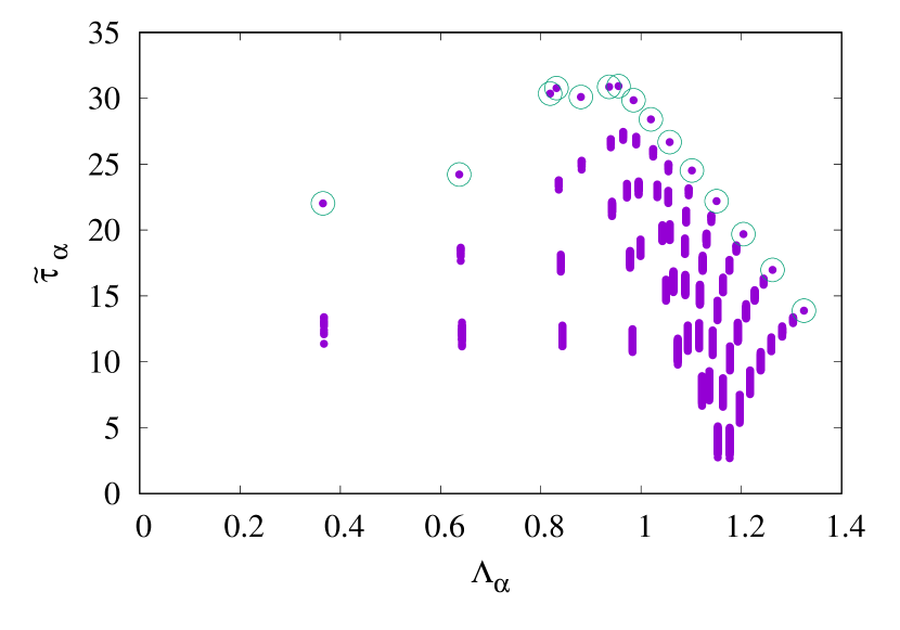
Here we diagonalize the generator of the master equation for the probability distribution over all microscopic states, which we call “the full generator”, and compare with the description using the collective variable . The result for , , , and is shown in Fig. 6. In the calculation, in order to avoid eigenvalue degeneracies, we introduced very weak inhomogeneity: is replaced by , where are independent random variables uniformly drawn from .
Figure 6 shows that the full generator contains all the eigenmodes of the generator of the master equation for the collective variable (shown by open circles). This is because the collective variable is completely decoupled from the other degrees of freedom in our model. In general, of course, coarse-grained description using collective variables is not exact.
Appendix B Non-ergodic phase
In the two-state model of interacting particles in the double-well potential, we have the non-ergodic phase for , where for . When , is a monotonic function of , whereas when , it becomes non-monotonic and has a local minimum, which is due to the mean-field character of the model. The non-ergodicity in the thermodynamic limit is a result of an extensive free energy barrier . The local minimum is interpreted as a metastable state in this case, and its lifetime grows with as .
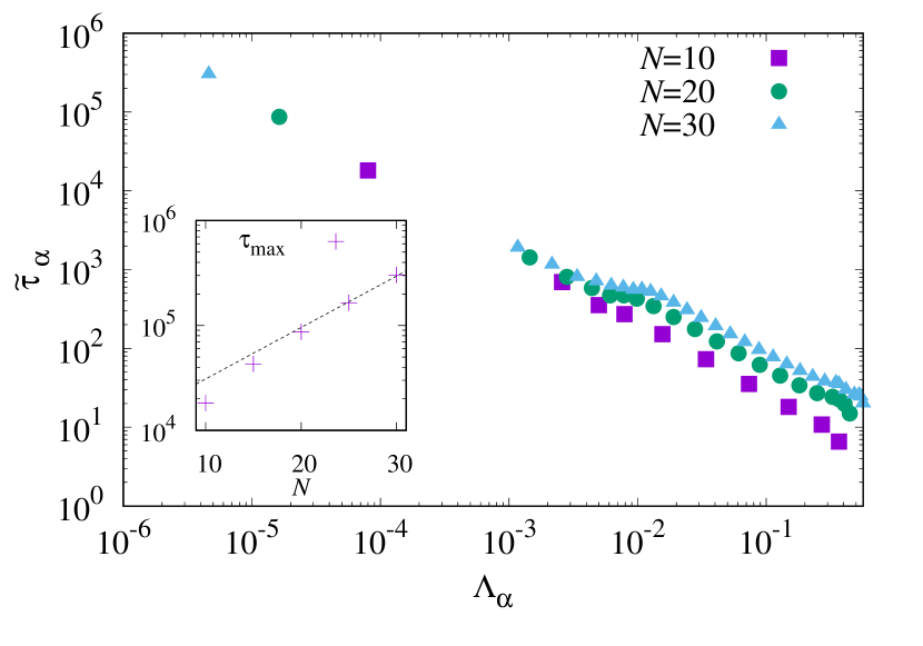
In the non-ergodic phase, metastability is fully explained by the gap closing of . We find that and . The corresponding maximum expansion coefficient does not grow with . This is explained by the fact that relaxation of a metastable state across the free energy barrier is regarded as a single-particle problem with the cooridinate . There is no “many-body” explosion in the relevant expansion coefficient. We show numerical results for , , and in Fig. 7. The maximum eigenmode relaxation time agrees with , where (see the inset of Fig. 7.
References
- Langer (1969) J. S. Langer, Statistical theory of the decay of metastable states, Ann. Phys. (N. Y). 54, 258–275 (1969).
- Langer (1974) J. S. Langer, Metastable states, Physica 73, 61 (1974).
- Penrose (1995) O. Penrose, Metastable decay rates, asymptotic expansions, and analytic continuation of thermodynamic functions, J. Stat. Phys. 78, 267–283 (1995).
- Bray and Moore (1980) A. J. Bray and M. A. Moore, Metastable states in spin glasses, J. Phys. C Solid State Phys. 13, L469 (1980).
- Biroli and Kurchan (2001) G. Biroli and J. Kurchan, Metastable states in glassy systems, Phys. Rev. E 64, 016101 (2001).
- Berthier and Biroli (2011) L. Berthier and G. Biroli, Theoretical perspective on the glass transition and amorphous materials, Rev. Mod. Phys. 83, 587–645 (2011), arXiv:1011.2578 .
- Baldwin et al. (2011) A. J. Baldwin, T. P. Knowles, G. G. Tartaglia, A. W. Fitzpatrick, G. L. Devlin, S. L. Shammas, C. A. Waudby, M. F. Mossuto, S. Meehan, S. L. Gras, J. Christodoulou, S. J. Anthony-Cahill, P. D. Barker, M. Vendruscolo, and C. M. Dobson, Metastability of native proteins and the phenomenon of amyloid formation, J. Am. Chem. Soc. 133, 14160–14163 (2011).
- Griffiths et al. (1966) R. B. Griffiths, C. Y. Weng, and J. S. Langer, Relaxation times for metastable states in the mean-field model of a ferromagnet, Phys. Rev. 149, 301–305 (1966).
- Lanford and Ruelle (1969) O. E. Lanford and D. Ruelle, Observables at infinity and states with short range correlations in statistical mechanics, Commun. Math. Phys. 13, 194–215 (1969).
- Note (1) See Refs. Langer (1969); Penrose (1995) for attempts to give a static characterization of finite-lifetime metastable states associated with first-order phase transitions via an analytic continuation of the thermodynamic function.
- Gaveau and Schulman (1998) B. Gaveau and L. S. Schulman, Theory of nonequilibrium first-order phase transitions for stochastic dynamics, J. Math. Phys. 39, 1517–1533 (1998).
- Bovier et al. (2000) A. Bovier, M. Eckhoff, V. Gayrard, and M. Klein, Metastability and small eigenvalues in Markov chains, J. Phys. A. Math. Gen. 33, L447 (2000).
- Macieszczak et al. (2016) K. Macieszczak, M. Guţă, I. Lesanovsky, and J. P. Garrahan, Towards a Theory of Metastability in Open Quantum Dynamics, Phys. Rev. Lett. 116, 240404 (2016), arXiv:1512.05801 .
- Rose et al. (2016) D. C. Rose, K. Macieszczak, I. Lesanovsky, and J. P. Garrahan, Metastability in an open quantum Ising model, Phys. Rev. E 94, 052132 (2016), arXiv:1607.06780 .
- (15) D. C. Rose, K. Macieszczak, I. Lesanovsky, and J. P. Garrahan, Hierarchical classical metastability in an open quantum East model, arXiv:2010.15304 .
- Frenkel (2013) D. Frenkel, Simulations: The dark side, Eur. Phys. J. Plus 128, 10 (2013).
- Fredrickson and Andersen (1984) G. H. Fredrickson and H. C. Andersen, Kinetic Ising model of the glass transition, Phys. Rev. Lett. 53, 1244–1247 (1984).
- Mori and Shirai (2020) T. Mori and T. Shirai, Resolving a Discrepancy between Liouvillian Gap and Relaxation Time in Boundary-Dissipated Quantum Many-Body Systems, Phys. Rev. Lett. 125, 230604 (2020), arXiv:2006.10953 .
- Haga et al. (2021) T. Haga, M. Nakagawa, R. Hamazaki, and M. Ueda, Liouvillian Skin Effect: Slowing down of Relaxation Processes without Gap Closing, Phys. Rev. Lett. 127, 070402 (2021), arXiv:2005.00824 .
- (20) J. Bensa and M. Znidaric, Fastest local entanglement scrambler, multistage thermalization, and a non-Hermitian phantom, arXiv:2101.05579 .
- Gaveau and Schulman (1987) B. Gaveau and L. S. Schulman, Dynamical metastability, J. Phys. A. Math. Gen. 20, 2865–2873 (1987).
- Note (2) If we choose another normalization condition for right eigenvectors, the criterion of the relaxation should be modified. For example, if we employ the normalization , we have , and hence the criterion of the relaxation should be with being a fixed constant. Accordingly, the formula (7) should also be modified. In other words, Eq. (7) is appropriate only for the normalization scheme (2).
- Ritort and Sollich (2003) F. Ritort and P. Sollich, Glassy dynamics of kinetically constrained models, Adv. Phys. 52, 219–342 (2003), arXiv:0210382 [cond-mat] .
- Cancrini et al. (2008) N. Cancrini, F. Martinelli, C. Roberto, and C. Toninelli, Kinetically constrained spin models, Probab. Theory Relat. Fields 140, 459–504 (2008).
- Note (3) At , the Hamiltonian vanishes and is a symmetric matrix. Even in this case, the many-body explosion of expansion coefficients occurs.
- TÇnase-Nicola and Kurchan (2004) S. TÇnase-Nicola and J. Kurchan, Metastable states, transitions, basins and borders at finite temperatures, J. Stat. Phys. 116, 1201–1245 (2004), arXiv:0311273 [cond-mat] .
- Kurchan and Levine (2011) J. Kurchan and D. Levine, Order in glassy systems, J. Phys. A Math. Theor. 44, 035001 (2011), arXiv:1008.4068 .
- Jack (2013) R. L. Jack, Counting metastable states in a kinetically constrained model using a patch repetition analysis, Phys. Rev. E 88, 062113 (2013).