Metamagnetic transition in the two $f$ orbitals Kondo lattice model

We first treat the effect of the Ising and Hund’s interactions in orbitals 1 and 2 in the presence of magnetic field.

$\displaystyle H_{f}\equiv H_{\mathrm{intersite}}+H_{\mathrm{local}}\,,$

(6)

where the different terms are defined above.

In a mean field decoupling , we introduce the effective field acting on electrons in orbital 1 and 2 respectively, $h_{w1}$ and $h_{w2}$. The purely $f$-orbital part of the Hamiltonian is thus approximated as:

$\displaystyle H_{f}\approx H^{\mathrm{MF}}_{f}\equiv E_{0}-\sum_{i}\left(\mathbf{h}_{w1}\cdot\mathbf{S}_{i1}+\mathbf{h}_{w2}\cdot\mathbf{S}_{i2}\right)\,,$

(7)

where $E_{0}=N\frac{J^{\prime}}{2}(m_{1}^{z})^{2}+NJ_{H}(m_{1}^{x}m_{2}^{x}+m_{1}^{z}m_{2}^{z})$ and $m_{1(2)}^{z}=\frac{1}{N}\sum_{i}\langle{S_{i1(2)}^{z}}\rangle$ and $m_{1(2)}^{x}=\frac{1}{N}\sum_{i}\langle{S_{i1(2)}^{x}}\rangle$ are the components of magnetization in the $z$ and $x$ directions. Note the redefinition $J^{\prime}=2zJ$, where $z$ is the number of nearest neighbors.

The effective fields are defined as

$\displaystyle\mathbf{h}_{w1}=\left({\begin{array}[]{c}h_{x}+J_{H}m_{2}^{x}\\ 0\\ h_{z}+J^{\prime}m_{1}^{z}+J_{H}m_{2}^{z}\end{array}}\right)\,,$

(11)

$\displaystyle\mathbf{h}_{w2}=\left({\begin{array}[]{c}h_{x}+J_{H}m_{1}^{x}\\ 0\\ h_{z}+J_{H}m_{1}^{z}\end{array}}\right)\,.$

(15)

We can also identify the angles of magnetization for both orbitals 1 and 2 with respect to x-direction:

	$\displaystyle\tan{\theta_{1}}$	$\displaystyle=\frac{m_{1}^{z}}{m_{1}^{x}}=\frac{h_{z}+J^{\prime}m_{1}^{z}+J_{H}m_{2}^{z}}{h_{x}+J_{H}m_{2}^{x}}\,,$		(16)
	$\displaystyle\tan{\theta_{2}}$	$\displaystyle=\frac{m_{2}^{z}}{m_{2}^{x}}=\frac{h_{z}+J_{H}m_{1}^{z}}{h_{x}+J_{H}m_{1}^{x}}\,.$		(17)

These definitions help us to have a more compact form for the set of self-consistent mean-field equations, that can be written as

	$\displaystyle m_{1}^{z}$	$\displaystyle=\frac{\sin{\theta_{1}}}{2}\tanh{\frac{\beta\|\mathbf{h}_{w1}\|}{2}}\,,$		(18)
	$\displaystyle m_{1}^{x}$	$\displaystyle=\frac{\cos{\theta_{1}}}{2}\tanh{\frac{\beta\|\mathbf{h}_{w1}\|}{2}}\,,$		(19)
	$\displaystyle m_{2}^{z}$	$\displaystyle=\frac{\sin{\theta_{2}}}{2}\tanh{\frac{\beta\|\mathbf{h}_{w2}\|}{2}}\,,$		(20)
	$\displaystyle m_{2}^{x}$	$\displaystyle=\frac{\cos{\theta_{2}}}{2}\tanh{\frac{\beta\|\mathbf{h}_{w2}\|}{2}}\,.$		(21)

The problem can be solved considering the external magnetic field in the $x$ - $z$ plane. However, as we will consider the Kondo coupling between the $f$ electrons in orbital 2 with the conduction electrons, the magnetization of orbital 2, $m_{2}^{f}$, has to be calculated self-consistently in the presence of Kondo coupling. This is presented below.

We now consider the full Hamiltonian defined by eq. (1), where the purely $f$-orbital part is approximated by the mean-field expression eq. (7):

$\displaystyle H\approx H^{\mathrm{MF1}}\equiv E_{0}+H^{\mathrm{MF}}_{f}+H_{\mathrm{Kondo}}+H_{c}~{},$

(22)

First it is necessary to make a basis change of the spin quantization axis: in the presence of the external magnetic field, the $f$ magnetic moments tend to point towards the direction of magnetic field, but they are not aligned with field since the Ising exchange acts as a local anisotropy (see above eqs. (18)-(21)). For this reason, we will change the quantization axis for the spins. We use the symbol tilde to represent this new quantization axis: $\tilde{z}$ and $\tilde{\sigma}$ correspond to the $z$ axis rotated by angle ${\theta_{2}}$ defined in the previous section. Invoking the spin rotational invariance of $H_{\mathrm{Kondo}}$ and $H_{c}$, the mean-field Hamiltonian is thus rewritten as

	$\displaystyle H^{\mathrm{MF1}}=$	$\displaystyle E_{0}+N\mu n_{c}-\mathbf{h}_{w1}\cdot\sum_{i}\mathbf{S}_{i1}-h_{w2}\sum_{i}S_{i2}^{\tilde{z}}$
		$\displaystyle+J_{K}\sum_{i}\tilde{\mathbf{S}}_{i2}\cdot\tilde{\mathbf{s}}_{i}+\sum_{{\bf k}\tilde{\sigma}}(\epsilon_{{\bf k}}-\mu)c_{{\bf k}\tilde{\sigma}}^{{\dagger}}c_{{\bf k}\tilde{\sigma}}~{}.$		(23)

The Kondo effect is treated within usual mean field approximation using fermionic representation of the spin operators :

	$\displaystyle S_{i2}^{\tilde{z}}=$	$\displaystyle\frac{1}{2}\left(f_{i2\tilde{\uparrow}}^{\dagger}f_{i2\tilde{\uparrow}}-f_{i2\tilde{\downarrow}}^{\dagger}f_{i2\tilde{\downarrow}}\right)$		(24)
	$\displaystyle S_{i2}^{\tilde{y}}=$	$\displaystyle\frac{i}{2}\left(f_{i2\tilde{\downarrow}}^{\dagger}f_{i2\tilde{\uparrow}}-f_{i2\tilde{\uparrow}}^{\dagger}f_{i2\tilde{\downarrow}}\right)$		(25)
	$\displaystyle S_{i2}^{\tilde{x}}=$	$\displaystyle\frac{1}{2}\left(f_{i2\tilde{\downarrow}}^{\dagger}f_{i2\tilde{\uparrow}}+f_{i2\tilde{\uparrow}}^{\dagger}f_{i2\tilde{\downarrow}}\right)~{},$		(26)

where the Abrikosov fermion annihilation (creation) operators $f_{i2\tilde{\sigma}}^{(\dagger)}$ satisfy the local constraints $\sum_{\tilde{\sigma}}f_{i2\tilde{\sigma}}^{\dagger}f_{i2\tilde{\sigma}}=1$. Within the mean-field approximation, this constraint is satisfied on average, $\sum_{i\tilde{\sigma}}\langle{f_{i2\tilde{\sigma}}^{\dagger}f_{i2\tilde{\sigma}}}\rangle=N$, by introducing an effective energy level $\epsilon^{f}_{2}$. Finally the mean-field approximations for the Hamiltonian give

	$\displaystyle H\approx H^{\mathrm{MF2}}$	$\displaystyle=E_{0}^{\mathrm{MF2}}-\mathbf{h}_{w1}\cdot\sum_{i}\mathbf{S}_{i1}+\sum_{i\tilde{\sigma}}\epsilon^{f}_{2\tilde{\sigma}}f_{i2\tilde{\sigma}}^{{\dagger}}f_{i2\tilde{\sigma}}$
		$\displaystyle+\sum_{i\tilde{\sigma}}\Lambda_{2}^{\tilde{\bar{\sigma}}}\Big{(}c_{i\tilde{\sigma}}^{{\dagger}}f_{i2\tilde{\sigma}}+f_{i2\tilde{\sigma}}^{{\dagger}}c_{i\tilde{\sigma}}\Big{)}+\sum_{{\bf k}\tilde{\sigma}}\epsilon_{{\bf k}}^{c}c_{{\bf k}\tilde{\sigma}}^{{\dagger}}c_{{\bf k}\tilde{\sigma}}\,,$		(27)

where $\lambda_{i2}^{\tilde{\sigma}}=\langle{f_{i2\tilde{\sigma}}^{{\dagger}}c_{i\tilde{\sigma}}}\rangle$ and

	$\displaystyle E_{0}^{\mathrm{MF2}}$	$\displaystyle=E_{0}+N\mu n_{c}-N\epsilon^{f}_{2}+J_{K}N\lambda_{2}^{\tilde{\uparrow}}\lambda_{2}^{\tilde{\downarrow}}\,,$		(28)
	$\displaystyle\epsilon^{f}_{2\tilde{\sigma}}$	$\displaystyle=\epsilon^{f}_{2}-\tilde{\sigma}h_{w2}\,,$		(29)
	$\displaystyle\Lambda_{2}^{\tilde{\sigma}}$	$\displaystyle=-\frac{J_{K}}{2}\lambda_{2}^{\tilde{\sigma}}\,,$		(30)
	$\displaystyle\epsilon_{{\bf k}}^{c}$	$\displaystyle=\epsilon_{{\bf k}}-\mu\,.$		(31)

$\tilde{\sigma}=\pm 1/2$ and $h_{w2}=\|\mathbf{h}_{w2}\|$. With the first mean-field approximation that we used, the momenta $\mathbf{S}_{i1}$ describing the local electronic orbital 1 are effectively decoupled from both the orbital 2 and the conduction electrons. However, the Hund interaction between orbitals 1 and 2 is still implicitly present through the effective fields $\mathbf{h}_{w1}$ and $\mathbf{h}_{w2}$ given by solving eqs. (11) and (15) and the self-consistent relations (18) and (21). The second mean-field approximation replaces the Kondo interaction by an effective hybridization between orbital 2 and conduction electrons. It describes qualitatively and quantitatively the Kondo-singlet correlations that can occur at low temperature. The mean-field Hamiltonian can be diagonalized using the space momentum representation ${\bf k}$:

$\displaystyle H^{\mathrm{MF2}}$

$\displaystyle=E_{0}^{\mathrm{MF2}}-\mathbf{h}_{w1}\cdot\sum_{i}\mathbf{S}_{i1}+\sum_{{\bf k}\tilde{\sigma}}\left(c_{{\bf k}\tilde{\sigma}}^{{\dagger}},f_{{\bf k}2\tilde{\sigma}}^{{\dagger}}\right)H_{{\bf k}\tilde{\sigma}}^{cf_{2}}\left(\begin{array}[]{c}c_{{\bf k}\tilde{\sigma}}\\ f_{{\bf k}2\tilde{\sigma}}\end{array}\right)~{},$

(35)

with

$\displaystyle H_{{\bf k}\tilde{\sigma}}^{cf_{2}}\equiv\left(\begin{array}[]{cc}\epsilon_{{\bf k}}^{c}&\Lambda_{2}^{\tilde{\sigma}}\\ {}{}\hfil&{}{}\hfil\\ \Lambda_{2}^{\tilde{\sigma}}&\epsilon^{f}_{2\tilde{\sigma}}\end{array}\right)~{}.$

(39)

From $H^{\mathrm{MF2}}$ and using the above expression of the block $H_{{\bf k}\tilde{\sigma}}^{cf_{2}}$, the one body Green’s functions for orbital 2 and conduction electrons can be written as

	$\displaystyle g_{{\bf k}\tilde{\sigma}}^{cc}(i\omega)$	$\displaystyle=\frac{i\omega-\epsilon^{f}_{2\tilde{\sigma}}}{(i\omega-\epsilon_{{\bf k}}^{c})(i\omega-\epsilon^{f}_{2\tilde{\sigma}})-(\Lambda_{2}^{\tilde{\bar{\sigma}}})^{2}}\,,$		(40)
	$\displaystyle g_{{\bf k}\tilde{\sigma}}^{f_{2}f_{2}}(i\omega)$	$\displaystyle=\frac{i\omega-\epsilon_{{\bf k}}^{c}}{(i\omega-\epsilon_{{\bf k}}^{c})(i\omega-\epsilon^{f}_{2\tilde{\sigma}})-(\Lambda_{2}^{\tilde{\bar{\sigma}}})^{2}}\,,$		(41)
	$\displaystyle g_{{\bf k}\tilde{\sigma}}^{cf_{2}}(i\omega)$	$\displaystyle=g_{{\bf k}\tilde{\sigma}}^{f_{2}c}(i\omega)=\frac{-\Lambda_{2}^{\tilde{\bar{\sigma}}}}{(i\omega-\epsilon_{{\bf k}}^{c})(i\omega_{n}-\epsilon^{f}_{2\tilde{\sigma}})-(\Lambda_{2}^{\tilde{\bar{\sigma}}})^{2}}\,.$		(42)

From the Green functions we can calculate the self-consistent parameters:

	$\displaystyle n_{\tilde{\sigma}}^{c}$	$\displaystyle=\sum_{{\bf k}}\int_{-\infty}^{\infty}d\omega f(\omega)\rho_{{\bf k}\tilde{\sigma}}^{c}(\omega)\,,$		(43)
	$\displaystyle n_{\tilde{\sigma}}^{f_{2}}$	$\displaystyle=\sum_{{\bf k}}\int_{-\infty}^{\infty}d\omega f(\omega)\rho_{{\bf k}\tilde{\sigma}}^{f_{2}}(\omega)\,,$		(44)
	$\displaystyle\lambda_{2}^{\tilde{\sigma}}$	$\displaystyle=\sum_{{\bf k}}\int_{-\infty}^{\infty}d\omega f(\omega)\rho_{{\bf k}\tilde{\sigma}}^{cf_{2}}(\omega)\,.$		(45)

where the the spectral density functions are

	$\displaystyle\rho_{{\bf k}\tilde{\sigma}}^{c}(\omega)$	$\displaystyle=-\frac{1}{\pi}\Im{\big{[}g_{{\bf k}\tilde{\sigma}}^{cc}(i\omega)\big{]}}\,,$		(46)
	$\displaystyle\rho_{{\bf k}\tilde{\sigma}}^{f_{2}}(\omega)$	$\displaystyle=-\frac{1}{\pi}\Im{\big{[}g_{{\bf k}\tilde{\sigma}}^{f_{2}f_{2}}(i\omega)\big{]}}\,,$		(47)
	$\displaystyle\rho_{{\bf k}\tilde{\sigma}}^{cf_{2}}(\omega)$	$\displaystyle=-\frac{1}{\pi}\Im{\big{[}g_{{\bf k}\tilde{\sigma}}^{cf_{2}}(i\omega)\big{]}}\,.$		(48)

The parameters defined in equations (43)(44)(45) are solved considering a square band (i.e., a constant density of states) for the conduction electrons. The only ${\bf k}$ dependence comes from the dispersion relation $\epsilon_{{\bf k}}$, in this way, the sum over ${\bf k}$ is changed by an integral over energy as $\sum_{{\bf k}}\rightarrow\int_{-D}^{D}\rho_{0}(\epsilon)d\epsilon$. The non-interacting conduction electrons density of states is taken as $\rho_{0}=1/2D$ in the interval $[-D:D]$. $D$ is the half of the value of the bandwidth.

Using the above expressions for the Green’s functions and invoking the relation eq. (31), the mean-field self-consistent equations can be rewritten as

$\displaystyle n_{\tilde{\sigma}}^{c}$

$\displaystyle=\rho_{0}\int_{-D}^{D}d\epsilon\frac{\left(E_{+}^{\tilde{\sigma}}(\epsilon)-\epsilon^{f}_{2\tilde{\sigma}}\right)f(E_{+}^{\tilde{\sigma}}(\epsilon))-\left(E_{-}^{\tilde{\sigma}}(\epsilon)-\epsilon^{f}_{2\tilde{\sigma}}\right)f(E_{-}^{\tilde{\sigma}}(\epsilon))}{\Delta E(\epsilon)}\,,$

(49)

$\displaystyle n_{\tilde{\sigma}}^{f_{2}}$

$\displaystyle=\rho_{0}\int_{-D}^{D}d\epsilon\frac{\left(E_{+}^{\tilde{\sigma}}(\epsilon)-\epsilon_{{\bf k}}^{c}\right)f(E_{+}^{\tilde{\sigma}}(\epsilon))-\left(E_{-}^{\tilde{\sigma}}(\epsilon)-\epsilon_{{\bf k}}^{c}\right)f(E_{-}^{\tilde{\sigma}}(\epsilon))}{\Delta E(\epsilon)}\,,$

(50)

$\displaystyle\Lambda_{2}^{\tilde{\sigma}}$

$\displaystyle=\frac{\rho_{0}J_{K}}{2}\Lambda_{2}^{\tilde{\sigma}}\int_{-D}^{D}d\epsilon\frac{f(E_{+}^{\tilde{\sigma}}(\epsilon))-f(E_{-}^{\tilde{\sigma}}(\epsilon))}{\Delta E(\epsilon)}\,.$

(51)

where $f(\omega)=(1+e^{\beta\omega})^{-1}$ denotes the Fermi-Dirac function, and

	$\displaystyle E_{\pm}^{\tilde{\sigma}}(\epsilon)$	$\displaystyle\equiv\frac{\epsilon+\epsilon^{f}_{2\tilde{\sigma}}\pm\sqrt{(\epsilon-\epsilon^{f}_{2\tilde{\sigma}})^{2}+4(\Lambda_{2}^{\tilde{\bar{\sigma}}})^{2}}}{2}\,,$		(52)
	$\displaystyle\Delta E(\epsilon)$	$\displaystyle\equiv E_{2}^{\tilde{\sigma}}(\epsilon)-E_{3}^{\tilde{\sigma}}(\epsilon)~{}.$		(53)

We note that the mean-field equation (51) has a trivial solution $\Lambda_{2}^{\tilde{\sigma}}=0$ which is realized in the non-Kondo phases where the local $f$ and the conduction electrons are decoupled. When a solution $\Lambda_{2}^{\tilde{\sigma}}\neq 0$ exists and is energetically stable, a Kondo phase is realized. On top of this usual mean-field description of Kondo effect, we also consider here the possibility of magnetic ordering, which may coexist or not with the Kondo effect. From equation (50) we can obtain the magnetization of orbital 2 in the rotated direction (noted with tilda), $M_{2}^{f\tilde{z}}=\frac{1}{2}(n_{\tilde{\uparrow}}^{f_{2}}-n_{\tilde{\downarrow}}^{f_{2}})$. However, this magnetization is in the direction of the effective field $h_{w2}$ and not in the original $z$ or $x$ directions. The magnetization in the initial cartesian coordinates is thus given by

	$\displaystyle m_{2}^{z}$	$\displaystyle=M_{2}^{f\tilde{z}}\sin{\theta_{2}}\,,$		(54)
	$\displaystyle m_{2}^{x}$	$\displaystyle=M_{2}^{f\tilde{z}}\cos{\theta_{2}}\,,$		(55)

where $\theta_{2}$ was defined previously in equation (17).

Finally, we can solve self-consistently our set of six equations (49), (50), (18), (54), and (51), and determine the parameters $\mu$, $\epsilon^{f}_{2}$, $m_{1}^{z}$, $m_{2}^{z}$, $\tilde{\lambda}_{2}^{\uparrow}$, and $\tilde{\lambda}_{2}^{\downarrow}$, respectively. We have checked the self-consistent solutions looking for the parameters that minimize the mean-field Hamiltonian presented in equation (35) for the case $T\rightarrow 0$. The numerical results are presented in the next section.

First we study here the effect of a magnetic field and Kondo coupling in the absence of both Hund and intersite interactions, $J_{H}=0$ and $J^{\prime}=0$. In this case the local spins $\mathbf{S}_{i1}$ are fully decoupled from the orbital 2 and the conduction electrons. The model corresponds to an usual Kondo lattice for orbital 2, and we use the Abrikosov fermions $f_{i2}$ to describe the local spins $\mathbf{S}_{i2}$. Since rotational symmetry is preserved at zero field when $J^{\prime}=0$, we arbitrarily choose the $x$-axis along the direction of the applied magnetic field.

The figure 2$(\mathbf{a})$ shows the variation of the effective Kondo hybridizations $\lambda_{\sigma}$ and the magnetizations for both orbitals as a function of the magnetic field $h_{x}$, for $J_{K}=1.0$ and $J=J_{H}=0$. Here, orbital 1 is fully decoupled from the other electrons, therefore in the ground state its magnetization saturates to its maximal value as soon as $h_{x}\neq 0$. The magnetization of orbital 2 is more interesting and we can identify three regimes depending on intensity of the applied magnetic field: at relatively small $h_{x}$, we find that $m_{2}^{x}$ increases linearly with $h_{x}$, revealing a Fermi-liquid regime with a finite susceptibility that correspond to the usual Kondo coherent regime. On the other side, the magnetization $m_{2}^{x}$ saturates to its maximal value when the applied field is higher than a critical value ${h_{K}^{\star}}$. ${h_{K}^{\star}}$ is defined as the critical field necessary to destroy the Kondo hybridization and it coincides with the saturation of $m_{2}^{x}$ only in some cases (see section 3.3). The intermediate regime of magnetic fields, above the linear response and below the critical value ${h_{K}^{\star}}$, we find a magnetization plateau at the value $m_{2}^{x}\approx(1-n_{c})/2$ independently from $h_{x}$ and $J_{K}$ as can be seen in figures 2(b) and 2(c).

The three magnetization regimes described above can be interpreted as follows: for relatively small $h_{x}$, the local Kondo spins $\mathbf{S}_{i2}$ and the conduction electrons form a coherent Kondo Fermi liquid state characterized by a constant susceptibility and a linear magnetization. The occurrence of an intermediate plateau regime at higher values of the field was predicted previously for a Kondo lattice (see Figure 5 in [46]). It can be explained using a strong Kondo coupling picture: independently from the magnetic field, in this Kondo phase a fraction $n_{c}$ of the Kondo spins are screened and form local Kondo singlets with the conduction electrons. The remaining fraction $1-n_{c}$ of unscreened Kondo spins can thus be magnetized without breaking the macroscopic coherent Kondo state. This intermediate Kondo regime with a magnetization plateau is energetically favorable as long as the Kondo singlet energy (typically the Kondo temperature $T_{K}$) is higher than the Zeeman energy (proportional to $h_{x}$).

This plateau corresponds to a Kondo phase with $\lambda_{\uparrow}$ and $\lambda_{\downarrow}$ slightly different from each other but both non-zero (see figure 2(${\mathbf{a}}$)). In the Kondo phase, $\lambda_{\uparrow}$ and $\lambda_{\downarrow}$ take relatively close values that differ as soon as $h_{x}$ is non-zero and both vanish above the same critical field ${h_{K}^{\star}}$ which marks the breakdown of Kondo effect.

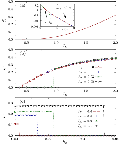
The variation of ${h_{K}^{\star}}$ is depicted in figure 3(a) and in its inset. After an exponential behavior ($\sim\exp(-a/J_{K})$) at small Kondo coupling, it goes linearly with $J_{K}$ for strong Kondo interaction. From the inset, it is possible to verify that the Kondo critical field scales as $T_{K}$ for $h_{x}=0$ [46]. The figures 3(b) and 3(c) present the variation of the $f-c$ effective hybridization $\lambda_{\uparrow}$ as a function of $J_{K}$ for fixed values of $h_{x}$, and as a function of $h_{x}$ for fixed values of $J_{K}$, respectively. We find that $\lambda_{\uparrow}$ vanishes at small $J_{K}$ as soon as $h_{x}$ is non-zero, it abruptly jumps to a finite value around a critical value of $J_{K}$ and then increases continuously with $J_{K}$. When fixing the Kondo coupling, we find that the effective hybridization is almost constant as $h_{x}$ increases and vanishes abruptly at $h_{x}\equiv h_{K}^{\star}$. This is consistent with the abrupt jump observed when increasing $J_{K}$, reflecting the fact that $h_{K}^{\star}$ depends on $J_{K}$ in a monotonous way.

Here, the effect of a magnetic field along the $x$ direction is analyzed by considering also the intersite Ising-like interaction $J^{\prime}$ for the orbital 1. The Hund’s coupling is not considered here, $J_{H}=0$. Therefore the orbital 1 is fully decoupled from the other electrons which, on their side, form a Kondo lattice system. The model for the orbital 2 and the conduction electrons is similar to the one discussed in section 3.1 and we thus choose here to fix $J_{K}=1.0$ which correspond to $h_{K}^{\star}\approx 0.036$. The evolution of the magnetizations of the two orbitals as well as the $f-c$ effective hybridization as a function of the magnetic field $h_{x}$ are depicted in figure 4. We consider that the intersite magnetic exchange between electrons in orbital 1 is of the same order of magnitude as the critical field $h_{K}^{\star}$. The resultas for $J^{\prime}=0.05$ in  4(a), and $J^{\prime}=0.1$ in  4(b) are presented in figure 4.

The Kondo lattice formed by electrons in the orbital 2 is discussed in detail in section 3.1 with the three regimes, linear, plateau, and saturation. We now focus on the analysis of orbital 1, which is saturated to its maximal value $\|\mathbf{m_{1}}\|=1/2$, but not necessarily in the same direction as $m_{2}$. The Ising-like interaction $J^{\prime}$ favors a magnetization along the $z$ direction, while the transverse magnetic field favors alignment along $x$. By exploiting the fact that orbital 1 is decoupled from other electrons we can solve exactly the mean-field equation for $\mathbf{m_{1}}$ at zero temperature. Indeed, for $J_{H}=0$ and with a field oriented along $x$ axis, Eq. 16 has two possible solutions: either $m_{1}^{z}=0$ and $m_{1}^{x}=1/2$, which is realized at sufficiently large field. Or $m_{1}^{x}=h_{x}/J^{\prime}$ and $m_{1}^{z}=\sqrt{\frac{1}{4}-\left(\frac{h_{x}}{J^{\prime}}\right)^{2}}$ at fields $h_{x}$ lower than a critical value $h_{M}^{\star}=J^{\prime}/2$. This linear increase of $m_{1}^{x}$ with $h_{x}$ is depicted in figure 4(a), corresponding to a gradual rotation of the magnetization until its complete alignment along $x$ axis at $h_{x}\geq h_{M}^{\star}$. The model parameters used for the plots in figure 4(a) correspond to $h_{M}^{\star}=0.025$, which is slightly lower than the other critical field $h_{K}^{\star}\approx 0.036$ characterizing the vanishing of the Kondo $f-c$ hybridization and the full magnetization of orbital 2. However, by increasing the value of the Ising interaction $J^{\prime}$, the alignment of $\mathbf{m_{1}}$ along $x$ axis can also be obtained for higher critical field, inside the non-Kondo regime ($h_{M}^{\star}>h_{K}^{\star}$), as can be seen in figure 4(b) .

We now extend our study by considering the effect of the transverse magnetic field in the presence of local Hund’s coupling and intersite Ising interaction. In this case, orbital 1 and 2 interact by the Hund’s coupling and orbital 2 is coupled with the conduction electrons by Kondo interaction. In the presence of magnetic field, the magnetization of orbital 2 will no longer be in the field direction because it is coupled to the magnetization of orbital 1. Moreover, the Weiss mean-field resulting from Hund’s coupling will add to the applied field and it is expected to weaken the effective Kondo hybridization , destroying it for a critical field smaller than ${h_{K}^{\star}}$ defined above.

The evolutions of the various mean-field parameters as functions of the magnetic field $h_{x}$ are depicted in figure 5. We consider two set of parameters corresponding to either $h_{M}^{\star}>h_{K}^{\star}$ (Figure 5$(\mathbf{a})$) or $h_{K}^{\star}>h_{M}^{\star}$ (Figure 5$(\mathbf{b})$) described previously for $J_{H}$.

The behaviors depicted in figure 5(a) for small $J_{H}=0.02$ is similar with the one depicted in figure 4(b) for $J_{H}=0$. For example, both plateau and saturated regimes are observed for the magnetization of orbital 2, but now for the modulus of $m_{2}$ (shown in Figure 6 $\mathbf{(a)}$). Here, the small but non-zero $z$-component comes from a combined effect of Hund’s coupling with orbital 1 together with the Ising intersite interaction ; the variation with field is no longer linear behavior as it was for $J_{H}=0.0$. Also, some slight discontinuities are observed for the magnetizations $m_{1}^{x}$ and $m_{1}^{z}$ at the critical field $h_{K}^{\star}$, which marks the vanishing of the Kondo $f-c$ hybridization.

The figure 5 $\mathbf{(b)}$ obtained for $J_{K}=1.3$ and $J_{H}=0.07$ shows an increase of $h_{K}^{\star}$ since the Kondo coupling is increased. The discontinuities of $m_{1}^{x}$ and $m_{1}^{z}$ are not observed, and the $z$-component of $\mathbf{m}_{2}$ is larger. Also, the stronger value of $J_{K}$ allows stabilization of the mixed state with a magnetic moments of orbital 1 completely aligned to the magnetic field $h_{x}$. The figure 5 ($\mathbf{c}$) is obtained for $J_{K}=1.0$ and $J_{H}=0.1$. The resulting Weiss field induced by the fully polarized orbital 1 on the orbital 2 has stronger intensity than the previous cases reported before.The presence of Ising interaction together with Hund’s coupling favors magnetizations aligned along $z$ direction for small $h_{x}$, while the alignment is along $x$ direction above a critical field $h_{M}^{\star}$. The rotations of the magnetizations induced by the field are continuous and gradual.

The variation of the magnetization at orbital 2 as a function of the transverse magnetic field and the number of conduction electron is depicted in figure 6. For the three values of $n_{c}$ shown in figure 6(a), we can see the presence of the plateau already discussed at $\sim(1-n_{c})/2$. In figure 6(b), the linear variation of $m_{2}$ is observed for some range of $n_{c}$, where the plateau is present.

The figure 7 shows the phase diagrams as a function of occupation number, $n_{c}$, and the transverse magnetic field, $h_{x}$, for fixed $J^{\prime}=0.1$ and four combinations of $J_{K}$ and $J_{H}$. Following the description made in the subsection 3.1, we can relate the different phases with the schematic pictures presented in figure 1. In the white part of Figure 7, the F1 phase is defined as a ferromagetic phase where the $z$ component of the magnetization is non-zero. In the yellow region, the F2 phase corresponds to a magnetization completely aligned with the applied field. It can be saturated for both orbitals, leading to the fully polarized state. In the red region, FK1 indicates a mixed state: ferromagnetic (non fully polarized) order and Kondo hybridization coexist. Another mixted state is obtained, FK2, which appears in the orange region: here, the magnetization oriented along $x$ direction coexists with Kondo hybridization. The two diagrams represented by figures 7$\mathbf{(a)}$ and $\mathbf{(c)}$, which mimic two different values of $J_{H}$, represent qualitatively similar situations: in both cases, FK1 can be present for sufficiently large value of electronic filling $n_{c}$ and small field; this phase is limited by the critical field $h_{K}^{\star}$ above which the field always abruptly destroys the Kondo hybridization. Also, here, an increase of $J_{H}$ results in a decrease of $h_{K}^{\star}$, which vanishes at small $n_{c}$ where non Kondo state can be formed. In all cases, a fully polarized non-Kondo state F2 is realized for strong applied manetic field. We now focus onto the diagrams obtained for larger values of Kondo interaction. In 7$\mathbf{(b)}$, an intermediate situation is observed with $J_{K}$ slightly stronger than the one in 7$\mathbf{(a)}$. In this case, a direct transition from FK1 to F2 may be realized by applying a magnetic field if $n_{c}$ is sufficiently large. Such a FK1-F2 transition corresponds to $h_{K}^{\star}=h_{M}^{\star}$ and, as a consequence, all parameters are expected to vary abruptly, especially magnetization (value and orientation), electronic density of states, Fermi-surface. Figure 7$\mathbf{(d)}$ depicts a situation obtained where both Kondo and Hund interactions are relatively stronger than in other figures. In this case, a cascade of transitions FK1-FK2-F2 can be induced by the magnetic field: as a first step, from FK1 to FK2, the magnetic field continuously turns the magnetization to $x$ direction, preserving continuously the non-zero Kondo hybridization just above $h_{M}^{\star}$. Then, in the intermediate Kondo phase FK2, the $x$ component of ${\bf m_{2}}$ reaches the plateau behaviour. The breakdown of Kondo effect can then be realized (FK2-F2 transition) at the critical field $h_{K}^{\star}>h_{M}^{\star}$.

References

- [1] G. Zwicknagl, A. N. Yaresko, P. Fulde, Microscopic description of origin of heavy quasiparticles in UPt 3, Physical Review B 65 (8) (2002) 081103. doi:10.1103/PhysRevB.65.081103.
- [2] G. Zwicknagl, A. Yaresko, P. Fulde, Fermi surface and heavy masses for UPd 2 Al 3, Physical Review B 68 (5) (2003) 052508. doi:10.1103/PhysRevB.68.052508.
- [3] P. Fulde, P. Thalmeier, G. Zwicknagl, Strongly correlated electrons, arXiv:cond-mat/0607165 (Jul. 2006). arXiv:cond-mat/0607165, doi:10.1016/S0081-1947(06)80003-2.
- [4] A. D. Huxley, Ferromagnetic superconductors, Physica C: Superconductivity and its Applications 514 (2015) 368–377. doi:10.1016/j.physc.2015.02.026.
- [5] D. Aoki, K. Ishida, J. Flouquet, Review of U-based Ferromagnetic Superconductors: Comparison between UGe 2 , URhGe, and UCoGe, Journal of the Physical Society of Japan 88 (2) (2019) 022001. doi:10.7566/JPSJ.88.022001.
- [6] A. C. Hewson, The Kondo Problem to Heavy Fermions, 1st Edition, Cambridge University Press, 1993. doi:10.1017/CBO9780511470752.
- [7] S. Doniach, Phase Diagram for the Kondo Lattice, in: R. D. Parks (Ed.), Valence Instabilities and Related Narrow-Band Phenomena, Springer US, Boston, MA, 1977, pp. 169–176. doi:10.1007/978-1-4615-8816-0_15.
- [8] Q. Si, F. Steglich, Heavy Fermions and Quantum Phase Transitions, Science 329 (5996) (2010) 1161–1166. doi:10.1126/science.1191195.
- [9] S. Kirchner, S. Paschen, Q. Chen, S. Wirth, D. Feng, J. D. Thompson, Q. Si, Colloquium : Heavy-electron quantum criticality and single-particle spectroscopy, Reviews of Modern Physics 92 (1) (2020) 011002. doi:10.1103/RevModPhys.92.011002.
- [10] V. S. Zapf, E. J. Freeman, E. D. Bauer, J. Petricka, C. Sirvent, N. A. Frederick, R. P. Dickey, M. B. Maple, Coexistence of superconductivity and antiferromagnetism in CeRh 1 - x Co x In 5, Physical Review B 65 (1) (2001) 014506. doi:10.1103/PhysRevB.65.014506.
- [11] R. Settai, H. Shishido, S. Ikeda, Y. Murakawa, M. Nakashima, D. Aoki, Y. Haga, H. Harima, Y. Onuki, Quasi-two-dimensional Fermi surfaces and the de Haas-van Alphen oscillation in both the normal and superconducting mixed states of CeCoIn 5, Journal of Physics: Condensed Matter 13 (27) (2001) L627–L634. doi:10.1088/0953-8984/13/27/103.
- [12] H. Shishido, R. Settai, D. Aoki, S. Ikeda, H. Nakawaki, N. Nakamura, T. Iizuka, Y. Inada, K. Sugiyama, T. Takeuchi, K. Kindo, T. C. Kobayashi, Y. Haga, H. Harima, Y. Aoki, T. Namiki, H. Sato, Y. Ōnuki, Fermi Surface, Magnetic and Superconducting Properties of LaRhIn 5 and CeTIn 5 (T: Co, Rh and Ir), Journal of the Physical Society of Japan 71 (1) (2002) 162–173. doi:10.1143/JPSJ.71.162.
- [13] H. Aoki, S. Uji, A. K. Albessard, Y. Ōnuki, Transition of f electron nature from itinerant to localized: Metamagnetic transition in CeRu 2 Si 2 studied via the de Haas–van Alphen effect, Physical Review Letters 71 (13) (1993) 2110–2113. doi:10.1103/PhysRevLett.71.2110.
- [14] R. Daou, C. Bergemann, S. R. Julian, Continuous Evolution of the Fermi Surface of CeRu 2 Si 2 across the Metamagnetic Transition, Physical Review Letters 96 (2) (2006) 026401. doi:10.1103/PhysRevLett.96.026401.
- [15] M. Güttler, K. Kummer, K. Kliemt, C. Krellner, S. Seiro, C. Geibel, C. Laubschat, Y. Kubo, Y. Sakurai, D. V. Vyalikh, A. Koizumi, Visualizing the Kondo lattice crossover in YbRh 2 Si 2 with Compton scattering, Physical Review B 103 (11) (2021) 115126. doi:10.1103/PhysRevB.103.115126.
- [16] N. B. Perkins, M. D. Núñez-Regueiro, B. Coqblin, J. R. Iglesias, The underscreened Kondo lattice model applied to heavy fermion uranium compounds, Physical Review B 76 (2007) 125101. doi:dx.doi.org/10.1103/PhysRevB.76.125101.
- [17] C. Thomas, A. S. da Rosa Simões, C. Lacroix, J. R. Iglesias, B. Coqblin, Effect of anisotropy in the S=1 underscreened Kondo lattice, Journal of Magnetism and Magnetic Materials 372 (2014) 247–252. doi:10.1016/j.jmmm.2014.07.028.
- [18] Ph. Nozières, A. Blandin, Kondo effect in real metals, Journal de Physique 41 (3) (1980) 193–211. doi:10.1051/jphys:01980004103019300.
- [19] M. Fidrysiak, D. Goc-Jagło, E. Kądzielawa-Major, P. Kubiczek, J. Spałek, Coexistent spin-triplet superconducting and ferromagnetic phases induced by Hund’s rule coupling and electronic correlations: Effect of the applied magnetic field, Physical Review B 99 (20) (2019) 205106. doi:10.1103/PhysRevB.99.205106.
- [20] A. B. Shick, W. E. Pickett, Spin-orbit coupling induced degeneracy in the anisotropic unconventional superconductor UTe 2, Physical Review B 100 (13) (2019) 134502. doi:10.1103/PhysRevB.100.134502.
- [21] S. S. Saxena, P. Agarwal, K. Ahilan, F. M. Grosche, R. K. Haselwimmer, M. J. Steiner, E. Pugh, I. R. Walker, S. R. Julian, P. Monthoux, G. G. Lonzarich, A. Huxley, I. Sheikin, D. Braithwaite, J. Flouquet, Superconductivity on the border of itinerant-electron ferromagnetism in UGe2, Nature 406 (6796) (2000) 587–92. arXiv:10949292, doi:10.1038/35020500.
- [22] D. Aoki, A. Huxley, E. Ressouche, D. Braithwaite, J. Flouquet, J.-P. Brison, E. Lhotel, C. Paulsen, Coexistence of superconductivity and ferromagnetism in URhGe, Nature 413 (6856) (2001) 613–616. doi:10.1038/35098048.
- [23] N. T. Huy, A. Gasparini, D. E. de Nijs, Y. Huang, J. C. P. Klaasse, T. Gortenmulder, A. de Visser, A. Hamann, T. Görlach, H. v. Löhneysen, Superconductivity on the Border of Weak Itinerant Ferromagnetism in UCoGe, Physical Review Letters 99 (6) (2007) 067006. doi:10.1103/PhysRevLett.99.067006.
- [24] R. Troć, Z. Gajek, A. Pikul, Dualism of the 5 f electrons of the ferromagnetic superconductor UGe 2 as seen in magnetic, transport, and specific-heat data, Physical Review B 86 (22) (2012) 224403. doi:10.1103/PhysRevB.86.224403.
- [25] J. Schoenes, B. Frick, O. Vogt, Transport properties of uranium monochalcogenide and monopnictide single crystals, Physical Review B 30 (11) (1984) 6578. doi:dx.doi.org/10.1103/PhysRevB.30.6578.
- [26] S. Ran, C. Eckberg, Q.-P. Ding, Y. Furukawa, T. Metz, S. R. Saha, I.-L. Liu, M. Zic, H. Kim, J. Paglione, N. P. Butch, Nearly ferromagnetic spin-triplet superconductivity, Science 365 (6454) (2019) 684–687. doi:10.1126/science.aav8645.
- [27] S. Sundar, S. Gheidi, K. Akintola, A. M. Côté, S. R. Dunsiger, S. Ran, N. P. Butch, S. R. Saha, J. Paglione, J. E. Sonier, Coexistence of ferromagnetic fluctuations and superconductivity in the actinide superconductor UTe 2, Physical Review B 100 (14) (2019) 140502. doi:10.1103/PhysRevB.100.140502.
- [28] D. Aoki, F. Honda, G. Knebel, D. Braithwaite, A. Nakamura, D. Li, Y. Homma, Y. Shimizu, Y. J. Sato, J.-P. Brison, J. Flouquet, Multiple Superconducting Phases and Unusual Enhancement of the Upper Critical Field in UTe 2, Journal of the Physical Society of Japan 89 (5) (2020) 053705. doi:10.7566/JPSJ.89.053705.
- [29] A. Miyake, Y. Shimizu, Y. J. Sato, D. Li, A. Nakamura, Y. Homma, F. Honda, J. Flouquet, M. Tokunaga, D. Aoki, Metamagnetic transition in heavy fermion superconductor UTe2, Journal of the Physical Society of Japan 88 (6) (2019) 063706. doi:10.7566/jpsj.88.063706.
- [30] Q. Niu, G. Knebel, D. Braithwaite, D. Aoki, G. Lapertot, M. Vališka, G. Seyfarth, W. Knafo, T. Helm, J.-P. Brison, J. Flouquet, A. Pourret, Evidence of Fermi surface reconstruction at the metamagnetic transition of the strongly correlated superconductor UTe 2, Physical Review Research 2 (3) (2020) 033179. doi:10.1103/PhysRevResearch.2.033179.
- [31] D. Aoki, A. Nakamura, F. Honda, D. Li, Y. Homma, Y. Shimizu, Y. J. Sato, G. Knebel, J.-P. Brison, A. Pourret, D. Braithwaite, G. Lapertot, Q. Niu, M. Vališka, H. Harima, J. Flouquet, Unconventional superconductivity in heavy fermion UTe2, Journal of the Physical Society of Japan 88 (4) (2019) 043702. doi:10.7566/jpsj.88.043702.
- [32] J. Ishizuka, S. Sumita, A. Daido, Y. Yanase, Insulator-Metal Transition and Topological Superconductivity in UTe 2 from a First-Principles Calculation, Physical Review Letters 123 (21) (2019) 217001. doi:10.1103/PhysRevLett.123.217001.
- [33] A. B. Shick, S.-i. Fujimori, W. E. Pickett, UTe 2 : A nearly insulating half-filled j = 5 2 5 f 3 heavy-fermion metal, Physical Review B 103 (12) (2021) 125136. doi:10.1103/PhysRevB.103.125136.
- [34] C. Lacroix, M. Cyrot, Phase diagram of the Kondo lattice, Physical Review B 20 (5) (1979) 1969–1976. doi:10.1103/PhysRevB.20.1969.
- [35] P. Fazekas, E. Müller-Hartmann, Magnetic and non-magnetic ground states of the Kondo lattice, Zeitschrift für Physik B Condensed Matter 85 (2) (1991) 285–300. doi:10.1007/BF01313231.
- [36] G.-B. Li, G.-M. Zhang, L. Yu, Kondo screening coexisting with ferromagnetic order as a possible ground state for Kondo lattice systems, Physical Review B 81 (9) (2010) 094420. doi:10.1103/PhysRevB.81.094420.
- [37] R. Peters, N. Kawakami, T. Pruschke, Spin-Selective Kondo Insulator: Cooperation of Ferromagnetism and the Kondo Effect, Physical Review Letters 108 (8) (2012) 086402. doi:10.1103/PhysRevLett.108.086402.
- [38] Y. Liu, G.-M. Zhang, L. Yu, Weak ferromagnetism with the Kondo screening effect in the Kondo lattice systems, Physical Review B 87 (13) (2013) 134409. doi:10.1103/PhysRevB.87.134409.
- [39] D. Golež, R. Žitko, Lifshitz phase transitions in the ferromagnetic regime of the Kondo lattice model, Physical Review B 88 (5) (2013) 054431. doi:10.1103/PhysRevB.88.054431.
- [40] C. Thomas, A. S. da Rosa Simões, J. R. Iglesias, C. Lacroix, N. B. Perkins, B. Coqblin, Application of the S = 1 underscreened Anderson lattice model to Kondo uranium and neptunium compounds, Physical Review B 83 (1) (2011) 014415. doi:10.1103/PhysRevB.83.014415.
- [41] B. H. Bernhard, C. Lacroix, Coexistence of magnetic order and Kondo effect in the Kondo-Heisenberg model, Physical Review B 92 (9) (2015) 094401. doi:10.1103/PhysRevB.92.094401.
- [42] K. Suzuki, K. Hattori, Ground-state phase diagram of the $S = 1$ one-dimensional Kondo lattice model with a uniaxial anisotropy under transverse fields, Journal of the Physical Society of Japan 88 (2) (2019) 024707. arXiv:1808.10142, doi:10.7566/JPSJ.88.024707.
- [43] K. Suzuki, K. Hattori, Superconducting correlations in the one-dimensional kondo lattice models under magnetic fields, Journal of the Physical Society of Japan 89 (3) (2020) 034703. doi:10.7566/jpsj.89.034703.
- [44] B. H. Bernhard, Metamagnetism and tricritical behavior in the Kondo lattice model, Physical Review B 106 (5) (2022) 054436. doi:10.1103/PhysRevB.106.054436.
- [45] F. Lévy, I. Sheikin, B. Grenier, A. D. Huxley, Magnetic Field-Induced Superconductivity in the Ferromagnet URhGe, Science 309 (5739) (2005) 1343–1346. doi:10.1126/science.1115498.
- [46] S. Burdin, V. Zlatić, Multiple temperature scales of the periodic Anderson model: Slave boson approach, Physical Review B 79 (11) (2009) 115139. doi:10.1103/PhysRevB.79.115139.
- [47] V. P. Mineev, Metamagnetic phase transition in the ferromagnetic superconductor URhGe, Physical Review B 103 (14) (2021) 144508. doi:10.1103/PhysRevB.103.144508.
- [48] F. Hardy, D. Aoki, C. Meingast, P. Schweiss, P. Burger, H. v. Löhneysen, J. Flouquet, Transverse and longitudinal magnetic-field responses in the Ising ferromagnets URhGe, UCoGe, and UGe 2, Physical Review B 83 (19) (2011) 195107. doi:10.1103/PhysRevB.83.195107.
- [49] A. Gourgout, A. Pourret, G. Knebel, D. Aoki, G. Seyfarth, J. Flouquet, Collapse of Ferromagnetism and Fermi Surface Instability near Reentrant Superconductivity of URhGe, Physical Review Letters 117 (4) (2016) 046401. doi:10.1103/PhysRevLett.117.046401.
- [50] A. Miyake, D. Aoki, J. Flouquet, Field Re-entrant Superconductivity Induced by the Enhancement of Effective Mass in URhGe, Journal of the Physical Society of Japan 77 (9) (2008) 094709. doi:10.1143/JPSJ.77.094709.
- [51] E. A. Yelland, J. M. Barraclough, W. Wang, K. V. Kamenev, A. D. Huxley, High-field superconductivity at an electronic topological transition in URhGe, Nature Physics 7 (11) (2011) 890–894. doi:10.1038/nphys2073.
- [52] D. Aoki, G. Knebel, J. Flouquet, Fermi Surface Instabilities in Ferromagnetic Superconductor URhGe, Journal of the Physical Society of Japan 83 (9) (2014) 094719. arXiv:1407.5799, doi:10.7566/JPSJ.83.094719.
- [53] S.-i. Fujimori, I. Kawasaki, A. Yasui, Y. Takeda, T. Okane, Y. Saitoh, A. Fujimori, H. Yamagami, Y. Haga, E. Yamamoto, Y. Ōnuki, Itinerant magnetism in URhGe revealed by angle-resolved photoelectron spectroscopy, Physical Review B 89 (10) (2014) 104518. doi:10.1103/PhysRevB.89.104518.