MetaDiff: Meta-Learning with Conditional Diffusion for Few-Shot Learning
Abstract
Equipping a deep model the ability of few-shot learning (FSL) is a core challenge for artificial intelligence. Gradient-based meta-learning effectively addresses the challenge by learning how to learn novel tasks. Its key idea is learning a deep model in a bi-level optimization manner, where the outer-loop process learns a shared gradient descent algorithm (called meta-optimizer), while the inner-loop process leverages it to optimize a task-specific base learner with few examples. Although these methods have shown superior performance on FSL, the outer-loop process requires calculating second-order derivatives along the inner-loop path, which imposes considerable memory burdens and the risk of vanishing gradients. This degrades meta-learning performance. Inspired by recent diffusion models, we find that the inner-loop gradient descent process can be viewed as a reverse process (i.e., denoising) of diffusion where the target of denoising is the weight of base learner but origin data. Based on this fact, we propose to model the gradient descent algorithm as a diffusion model and then present a novel conditional diffusion-based meta-learning, called MetaDiff, that effectively models the optimization process of base learner weights from Gaussian initialization to target weights in a denoising manner. Thanks to the training efficiency of diffusion models, our MetaDiff does not need to differentiate through the inner-loop path such that the memory burdens and the risk of vanishing gradients can be effectively alleviated for improving FSL. Experimental results show that our MetaDiff outperforms state-of-the-art gradient-based meta-learning family on FSL tasks.
1 Introduction
With a large number of labeled data, deep learning techniques have shown superior performance and made breakthrough on various tasks. However, collecting such much data may be impractical or very difficult on some applications such as drug screening (Altae-Tran et al. 2017) and cold-start recommendation (Vartak et al. 2017). Inspired by the fast learning abaility of humans, i.e., humans can quickly learn a new concept or task from only very few examples, few-shot learning (FSL) has been proposed and has gained wide attention. It aims to learn transferable knowledge from data-ubundant base classes and then assist novel class prediction with few labeled examples (Wang et al. 2020).


To address this FSL problem, meta-learning (Rusu et al. 2018) has been proposed, which constructs a large number of base tasks from these base classes and then leverages it to learn task-agnostic meta knowledge for assisting novel class learning. Among these methods, gradient-based meta-learning methods are gaining increased attention, with its potential on generalization. This type of methods aims to learn a sample-efficient gradient descent algorithm (called meta-optimizer) by directly modeling its initialization (Finn et al. 2017), learning rate (Baik et al. 2020), or update rule (Ravi and Larochelle 2017) as a shared meta parameter and then learning it in a bi-level (i.e., outer-loop and inner-loop) optimization manner. Here, the outer-loop process accounts for learning a task-agnostic meta parameter for meta-optimizer, while the inner-loop process leverages the meta-optimizer to learn a task-specific base learner with few gradient updates. Although these methods have shown superior performance, the outer-loop process requires backpropagation along inner-loop optimization path and calculating second-order derivatives for learning meta-optimizer such that the significant memory overhead and risk of vanishing gradient is imposed during training (Rajeswaran et al. 2019). This degrades meta-learning performance (Nichol, Achiam, and Schulman 2018). Some works attempt to address this issue but from the perspective of gradient approximate estimations (Rajeswaran et al. 2019; Nichol, Achiam, and Schulman 2018), which would introduce an estimation error into the gradient (i.e., meta-gradient) for outer-loop optimization, and hamper its generalization ability.
Inspired by recent diffusion models (Ho, Jain, and Abbeel 2020), we also focus on gradient-based meta-learning with its good generalization but present a new diffusion perspective to model gradient descent algorithm. It does not need to differentiate through inner-loop, such that the above issues of memory burden and vanishing gradients can be alleviated for improving meta-learning. Specifically, as shown in Figures 1(a) and 1(b), we find that 1) the optimizaton process of gradient descent algorithm (see Figure 1(a)) is very similar to the denoising process of diffusion models from a Gaussion noise to a target variable (see Figure 1(b)). The key difference is that the denoising variable is model weight in gradient descent algorithm but origin image data in diffusion models; And 2) the latter is actually a generalized and learnable version of the former with weight momentum update and uncertainty estimation (see Section 4.1). In other words, the optimization process of gradient descent algorithm can be described as: given a randomly initial weight, the target weight is finally obtained by gradually removing its noise.
Based on this fact, we propose a novel meta-learning with conditional diffusion, called MetaDiff. As shown in Figure 1(c), our idea is regarding the weight of base learner as a denoising variable, and then modeling the gradient descent algorithm as a diffusion model and learning it in a diffusion manner. Its key challenge of achieveing the above idea is how to predict the diffused noise of model weights at each time step with few labeled samples for a base learner. To address this challenge, we take few labeled samples as the condition of diffusion models and carefully design a gradient-based task-conditional UNet for noise prediction. Different from previous gradient-based meta-learning methods that learn the meta-optimizer in a bi-level optimization manner, our MetaDiff learns it in a diffusion manner. Thanks to its training efficiency and robustness, more superior meta-learning performance can be achieved for improving FSL.
Our main contributions can be summarized as follows:
-
•
We are the first to reveal the close connection between gradient descent algorithm and diffusion models. From workflow, we find that the optimization process of gradient descent algorithm is very similar to the denoising process of diffusion models. After theoretical analysis, the denoising process of diffusion models is actually a generalized and learnable gradient descent algorithm with weight momentum updates and uncertainty estimation.
-
•
Based on this fact, we propose a novel diffusion-based meta-learning for FSL. In particular, a gradient-based conditional UNet is designed as our meta-learner for noise prediction. Thanks to diffusion training efficiency, the issue of memory burden and vanishing gradients can be effectively alleviated for improving meta-learning.
-
•
We conduct comprehensive experiments on two public data sets, which verify the effectivenss of our MetaDiff.
2 Related Work
2.1 Meta-Learning
Few-shot learning (FSL) is a challenging task, which aims to recognize novel classes with few examples (Chen et al. 2021, 2019). To address this problem, meta-learning is proposed, which aims to learn to quickly learn novel tasks with few examples (Flennerhag et al. 2019; Zhu and Koniusz 2023). The core idea is learning task-agnostic meta knowledge from a large number of similar tasks and then leveraging it to assist the learning of novel tasks. From the type of meta-knowledge, these existing meta-learning methods can be roughly grouped into three groups. The metric-based methods (Snell et al. 2017; Vinyals et al. 2016; Zhang et al. 2021a, 2022a, 2022c, 2022b, 2023a) regard the metric space or metric strategy as meta knowledge and perform the novel class prediction in a nearest-prototype manner. The model-based methods (Hou et al. 2019; Zhmoginov, Sandler, and Vladymyrov 2022; Li et al. 2019) regard a black-box model as meta knowledge, which leverages it and few data to directly predict model weights or test sample labels. The gradient-based methods (Rusu et al. 2018; Lee et al. 2019; Rajeswaran et al. 2019; Nichol, Achiam, and Schulman 2018; Von Oswald et al. 2021; Raghu et al. 2020; Zhang et al. 2023b) regard the gradient-based optimization algorithm as meta knowledge, which learn to model its hyperparameters (i.e., learning rate (Baik et al. 2020), loss function (Baik et al. 2021), initialization (Finn et al. 2017), preconditioner (Kang et al. 2023), or updata rules (Deleu et al. 2022; Ravi and Larochelle 2017)) such that the base learner can be quickly learned with few gradient updates.
We focus on the gradient-based meta-learning due its good generalization. However, different from existing methods, we presents a new diffusion perspective to model meta-optimizer, which does not need to differentiate through inner-loop path such that the issues of memory burdens and vanishing gradients can be alleviated for improving FSL.
2.2 Diffusion Models
Diffusion model (Ho, Jain, and Abbeel 2020; Nichol and Dhariwal 2021) is a popular type of deep generative models, which models and learns the generation process of target data from random Gaussion noises in a forward diffusion and reverse denoising manner. With the superior properties of diffusion models, the diffusion models have been widely exploited on various vision (Lugmayr et al. 2022) and multi-modal tasks (Rombach et al. 2022; Kawar et al. 2023; Kumari et al. 2023) and achieved remarkable performance improvement. However, there is very few works (i.e., (Roy et al. 2022) and (Hu et al. 2023)) to explore diffusion models for FSL. Specifically, in (Roy et al. 2022), Roy et al. introduce class names as priors and then leverage it and a text2image diffusion model to generate more images for alleviating the data-scarcity issue of FSL. Instead of using text2image diffusion models, Hu et al. (Hu et al. 2023) employ a image2image diffusion model and leverage it to generate more high-similarity pseudo-data for improving FSL.
Different from existing methods that regarding the diffusion model as a component of data augmentation, we find that the gradient descent process is similar to the denoising process, thus we propose to model the gradient descent algorithm as a diffusion model. We note that a concurrent working with our MetaDiff is ProtoDiff (Du et al. 2023). However, different from ProtoDiff that focuses on metric-based meta-learning (i.e., rectifying prototype bias), we target at gradient-based meta-learning, and first reveal the close connections between gradient descent algorithm and diffusion models. Then, a new diffusion-based meta-optimizer is presented for fast adaptation of base-learner.
3 Problem Definition and Preliminaries
3.1 Problem Definition
For a -way -shot FSL problem, it consists of two datasets, i.e., a base class dataset and a novel class dataset . The base class dataset consists of abundant labeled data from base class , which is used for assisting the classifier learning of novel classes. The novel class dataset contains two sub datasets from novel classes , i.e., a training set (call support set ) that consists of classes and samples per class and a test set (call query set ) consisting of unlabeled samples.
Our goal is that leveraging the base class dataset to learn a good meta-optimizer such that the classifier can be quickly learned from few labeled data (i.e., the support set ) to perform the novel class prediction for query set .
3.2 Preliminaries
Diffusion Models. Diffusion models aim to model a probability transformation from a prior Gaussian distribution to a target distribution . It consists of two processes, i.e., a diffusion (also called forward) process and a denoising (also called reverse) process.
1) The diffusion process aims to iteratively add a noise from a Gaussian distribution to a target data to transform into . The final tends to become a sample point from the prior distribution when the number of iterations tends to big enough. The diffusion process aims to learn a noise prediction model for estimating the added noise at time from , which is then used to recovery the target data in denoising process. The training object is as follows:
| (1) |
where denotes a mean squared error loss. It is worth noting that the above training object defined in Eq. (1) can be performed at any time step without the iterations of adding noise due to its good closed form at any time step . That is,
| (2) | ||||
where is a variance hyperparameter.
2) The denoising process is reverse process of diffusion. Based on the learned noise prediction model , given a start noise , we can iteratively remove its fraction of noises at each time and finally recovery the target data from the noisy data . That is,
| (3) |
where is a variance hyperparameter, which is theoretically set to in most existing diffusion works (Ho, Jain, and Abbeel 2020; Nichol and Dhariwal 2021).
Gradient Descent Algorithm (GDA). GDA is a family of optimization algorithm, which aims to optimize model weights by following the opposite direction of gradient. Formally, let denotes the weights of a base learner and be its differentiable loss function, and be its weight gradient, during performing gradient descent algorithm. The overall optimization process of GDA can be summaried as iteratively performing Eq. (4), that is,
| (4) |
where is an initial weight, i.e., a Gaussian noise in origin gradient descent algorithm; and denotes a learning rate. Due to the data scarcity issue in FSL, directly employing the Eq. (4) to learn a base learner would result in an overfitting issue. To address this issue, gradient-based meta-learning attempts to learn a GDA in a bi-level optimization (i.e., outer-loop and inner-loop) manner by modeling its hyperparameters (e.g., initial weight or learning rate ) as meta-knowledge for improving FSL. However, some studies (Rajeswaran et al. 2019) show the outer-loop process requires backpropagation along inner-loop optimization path such that the risk of vanishing gradient is imposed, which degrades meta-learning performance. In this paper, we propose a diffusion perspective to address this issue.

4 Methodology
4.1 Connection: Diffusion Models vs GDA
As introduced in Section 3.2, we can describe the process of denoising and gradient descent process as follows: 1) given a noise data , the denoising process iteratively performs Eq. (3) to obtain a latent sequence . As a result, a target data can be recoveried from a Gaussian noise ; and 2) given a randomly initial wight , the gradient descent process of GDA iteratively performs Eq. (4) to a latent sequence . As a result, an optimizal weight can be obtained from a random weight . We can see that the denoising process of diffusion models and gradient descent process of GDA are very similar in workflow. This inspires us to think about what is the close connection between the two methods in theory. Let’s take a closer look on Eqs. (3) and (4), Eq. (3) first can be simplifed as:
| (5) | ||||
Let denotes the Term 1, be the Term 2, be the Term 3 of Eq. (5), respectively. The Eq. (5) can be simplifed as:
| (6) |
Due to (), we can transform Eq. (6) as follows:
| (7) | ||||
where is denoising term, denotes a momentum update term with hyperparameter (also called exponentially weighted moving average), and is a uncertain term. Comparing Eqs. (4) and (7), we can see that the gradient decent process defined in Eq. (4) is equivalent to the of Eq. (7), which means that Eq. (4) is a special case of denoising process described in Eq. (7) when the is set to one (i.e., ), the is regarded as a hyperparameter, and the is set to zero. In particular, it is worth noting that the predicted variable of noise prediction model is actually the gradient (i.e., ) of model weights. In other words, the denosing process defined in Eq.(7) can be viewed as a generalized and learnable gradient descent algorithm defined in Eq.(4), i.e., a learnable gradent descent algorithm with weight momentum updates and uncertainty estimation where controls the weight of momentum updates, is a learning rate, and is the degree of uncertainty.
Why set parameters (, , and ) by following Eq. 5? Instead of using manual setting or model learning manner like existing meta-optimizers to set hyperparameters , , and , respectively, the diffusion models unify the parameter settings by theoretical deduction, i.e., , , and where , , and is experimentally set in linear decreasing manner from a small value (e.g., ) to a large value (e.g., 0.02). The goal of such setting is to ensure that denoising and diffusion processes have approximately the same functional form and the efficiency and robustness of diffusion training (i.e., the training objective defined in Eq. (1) can be performed at any time step without the iterations from to ).
4.2 Meta-Learning with Conditional Diffusion
Inspired by the above analysis, we find that the diffusion model is a generalized and learnable form of GDA and its hyperparameter setting have rigorous theoretical derivation, which enables its inspiring advantage (i.e., generation robustness and training efficiency). Based on this, we attempt to leverage a diffusion model to model GDA and then present a new meta-optimizer, i.e., MetaDiff, for fast adaptation of base-learner. It does not need to differentiate through inner-loop path, such that the memory burden and risk of vanishing gradients can be alleviated for improving FSL.
Overall Framework. The overall framework of our MetaDiff on FSL is presented in Figure 2(a), which consists of an embedding network with parameters , a base learner with parameters , and a MetaDiff meta-optimizer with meta parameters . Here, the embedding network aims to encode each support/query image as a -dim feature vector. Inspired by prior meta-learning works (Deleu et al. 2022; Lee et al. 2019), we assume that the embedding network is shared across tasks, which can be obtained by using a simple pretraining manner on entire base class classification task (Chen et al. 2021, 2019). The base learner is a simple linear or prototype classifer (the prototype classifer is used in this paper due it good performance), which is a task-specific and needs to be adapted starting at some Gaussian initialization . The MetaDiff is a meta-optimizer, which takes the features and labels of all support samples as inputs and then learns a target weights for base learner from initial weights in a denoising manner (see Figure 2(b)).
Specifically, given a -way -shot FSL task, we first leverage the embedding network to encode the feature for each support/query image . Then, we randomly initialize a weight for the base learner , and design a task-conditional UNet (i.e., the noise prediction model ) that regards the features and labels of all support sample as task condition, to estimate the noise to be removed at time . After that, we take the weight as the denoising variable and iteratively perform the denoising process from to , that is,
| (8) |
Note that we remove the uncertainty term (i.e., ) for deterministic estimation during inference. After iteratively perform step, the target weight can be obtained as the optimal weight for base learner . Finally, we perform class prediction of each query image by using the learned optimal base learner . That is,
| (9) |
Here, we only introduce the inference workflow of our MetaDiff-based FSL framework, which is summaried in Algorithm 2. Next, we will introduce the design details of our key component, i.e., the task-conditional UNet .
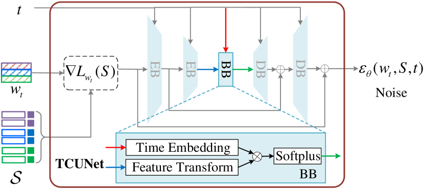
Task-Conditional UNet (TCUNet). The task-conditional UNet (TCUNet) is the key component in our MetaDiff meta-optimizer, which takes the features and labels of all support samples , time step , and the weight of base learner as inputs. It aims to estimate the noise to be remove for the weight of base learner at each time step . We attempt to use a general conditional UNet like (Rombach et al. 2022) for implementing TCUNet . However, we find that such general conditional UNet does not work in our MetaDiff, which inspires us to think deeply the rationale of the noise prediction model in our MetaDiff meta-optimizer. As analyzed in Section 4.1, we can see that the goal of noise prediction model is actually equivalent to predict gradient in meta-optimizer (see Eqs. (4) and (7)).
Based on this find, as shown in Figure 3, we design a task-conditional UNet from the perspective of gradient estimation as the noise prediction model . The key idea is predicting noise from the view of gradient estimation instead of a general black-box manner like (Rombach et al. 2022). Specifically, given a base learner weight at time and all features and labels of support samples , we first leverage the base learner with model weights to compute the loss of of all support samples. That is,
| (10) |
where is the number of support samples and is a loss function. Instead of cross-entropy loss, we employ a simple L2 loss to implement the , that is,
| (11) |
where is the class prototype of label . The intuition of such design is moving the class prototype towards the center of all labeled sample for each class , which is more matching for the rationale of prototype classifier. Then, the gradient regarding weights can be obtained as the initial noise estimation for the base learner at time . To obtain more accuracy noise estimation, we take the initial noise estimation as inputs and then design a conditional UNet fusing time embedding to predict the noise to be remove at time for base learner .
| Method | Adaptation Type | Backbone | miniImagenet | tieredImagenet | ||
| 5-way 1-shot | 5-way 5-shot | 5-way 1-shot | 5-way 5-shot | |||
| iMAML(Rajeswaran et al. 2019) | All | Conv4 | ||||
| ALFA (Baik et al. 2020) | All | Conv4 | ||||
| MeTAL (Baik et al. 2021) | All | Conv4 | ||||
| MetaSGD + SiMT (Tack et al. 2022a) | All | Conv4 | ||||
| GAP (Kang et al. 2023) | All | Conv4 | ||||
| ANIL (Raghu et al. 2020) | only CH | Conv4 | ||||
| COMLN (Deleu et al. 2022) | only CH | Conv4 | ||||
| MetaQDA (Zhang et al. 2021b) | only CH | Conv4 | ||||
| MetaDiff (ours) | only CH | Conv4 | 55.06 0.81 | 73.18 0.64 | 57.77 0.90 | 75.46 0.69 |
| ALFA (Baik et al. 2020) | All | ResNet12 | ||||
| MAML+SiMT (Tack et al. 2022b) | All | ResNet12 | 62.05 0.39 | 78.77 0.45 | 63.91 0.32 | 77.43 0.47 |
| LEO (Rusu et al. 2018) | only CH | WRN-28-10 | ||||
| Meta-Curvature(Park and Oliva 2019) | only CH | WRN-28-10 | ||||
| ANIL(Raghu et al. 2020) | only CH | ResNet12 | ||||
| COMLN (Deleu et al. 2022) | only CH | ResNet12 | 59.26 0.65 | 77.26 0.49 | 62.93 0.71 | 81.13 0.53 |
| ClassifierBaseline (Chen et al. 2021) | only CH | ResNet12 | 61.22 0.84 | 78.72 0.60 | 69.71 0.88 | 83.87 0.64 |
| MetaQDA (Zhang et al. 2021b) | only CH | ResNet18 | 65.12 0.66 | 80.98 0.75 | 69.97 0.52 | 85.51 0.58 |
| MetaDiff (ours) | only CH | ResNet12 | 64.99 0.77 | 81.21 0.56 | 72.33 0.92 | 86.31 0.62 |
As shown in Figure 3, the UNet consists of two encoder blocks (EB), a bottle block (BB) and two decoder blocks (DB). At each encoder step, we halve the number of input features and then remain unchanged at bottle step, but the number of features is doubled at each decoder step. The details of each encoder, bottle, decoder block are all similar, which contains a feature transform layer, a time embedding layer, and a ReLU activation layer. Note that we remove the ReLU activation layer in the final decoder block for estimating gradients. At each block, its output is obtained by first feeding the output of previous block and time step into the feature transform and time embedding layers, respectively, and then fusing them in an element-by-element product manner, finally followed by a softplus activation.
Meta-Learning Objective. Different from previous gradient based meta-learning methods that learn a meta-optimizer in a bi-level optimization manner, as shown in Figure 2(b), we employ a diffusion process to train our MetaDiff. However, unlike existing diffusion models (Ho, Jain, and Abbeel 2020) where the target data is known (i.e., origin images), the target variable of our MetaDiff is model weight (i.e., ) of base learner which is unknown. Thus, a key challenge of training our MetaDiff is how to obtain a large number of target weight for base learner .
To this end, we follow episodic training strategy (Vinyals et al. 2016) and construct a large number of -way -shot tasks from base class dataset . Then, given a constructed -way -shot tasks , based on its origin label of each class in the base classes , we extract all samples that belongs to the origin label of each class from the base class dataset , as the auxiliary dataset . The labeled data is very sufficient in the auxiliary dataset because it contains all labeled data belonging to class in , thus we can leverage it to learn a base learner such that the target weight can be obtained for each task . Finally, we leverage the target weight of all constructed tasks to train our MetaDiff meta-optimizer in a diffusion manner. That is,
| (12) |
During training, our MetaDiff does not require backpropagation along the inner-loop optimization path and calculating second-order derivatives for learning meta-optimizer such that the memory overhead and the risk of vanishing gradient can be effectively alleviated for improving FSL. The complete diffusion procedure is summaried in Algorithm 1.
5 Experiments
5.1 Datasets and Settings
MiniImagenet. It is a subset from ImageNet, which contains 100 classes and 600 images per class. Following (Lee et al. 2019), we split it into three sets, i.e., 64, 16, and 20 classes for training, validation, and test, respectively.
TieredImagenet. It is also a ImageNet subset but larger, which has 608 classes and 1200 images per class. Following (Lee et al. 2019), it is splited into 20, 6, and 8 high-level classes for training, validation, and test, respectively.
| Method | 5-way 1-shot | 5-way 5-shot | |
| (i) | Baseline (Standard GDA) | 60.53 0.86 | |
| (ii) | Replacing by Momentum GDA | 62.03 0.82 | 78.28 0.56 |
| (iii) | Replacing by ANIL | 60.77 0.82 | 77.34 0.64 |
| (iv) | Replacing by MetaLSTM | 63.56 0.81 | 79.90 0.59 |
| (v) | Replacing by ALFA | 63.92 0.82 | 80.01 0.61 |
| (vi) | Replacing by Our MetaDiff | 64.99 0.77 |
| Method | 5-way 1-shot | 5-way 5-shot | |
| (i) | TCUNet | 64.99 0.77 | 81.21 0.56 |
| (ii) | Replacing L2 loss | 62.92 0.79 | 80.92 0.56 |
| (iii) | w/o UNet | 62.72 0.84 | 80.72 0.55 |
5.2 Implementation Details
Network Details. We use Conv4 and ResNet12 as the embedding network , which are same to previous gradient-based meta-learning methods (Kang et al. 2023; Lee et al. 2019; Deleu et al. 2022) and delivers 128/512-dim vector for each image. In our task-conditional UNet, for encoder blocks, we use a linear layer with 512/256-dim inputs and 256/128-dim outputs to implement its feature transform layer, and a linear layer with 32-dim inputs and 256/128-dim outputs as its time embedding layer. For bottle blocks, we use a linear layer with 128-dim inputs and outputs to implement its feature transform layer, and a linear layer with 32-dim inputs and 128-dim outputs as its time embedding layer. For decoder blocks, we use a linear layer with 128/256-dim inputs and 256/512-dim outputs to implement its feature transform layer, and a linear layer with 32-dim inputs and 256/512-dim outputs as its time embedding layer.
Training Details. During training, we train our MetaDiff meta-optimizer 30 epochs (10000 iterations per epoch) using Adam with a learning rate of 0.0001 and a weight decay of 0.0005. Following the standard setting of diffusion models in (Ho, Jain, and Abbeel 2020), we set the number of denoising iterations to 1000 (i.e., is used).
| Method | 5-way 1-shot | 5-way 5-shot | |
| (i) | Prototype Classfier (ALFA) | 63.92 0.82 | 80.01 0.61 |
| Prototype Classfier (MetaDiff) | 64.99 0.77 | 81.21 0.56 | |
| (ii) | Linear Classfier (ALFA) | 62.09 0.84 | 78.13 0.59 |
| Linear Classfier (MetaDiff) | 62.72 0.89 | 80.19 0.57 |
5.3 Experimental Results
Our MetaDiff falls into the type of gradient-based meta-learning, thus we mainly select various state-of-the-art gradient-based meta learning methods as our baselines. We evaluate our MetaDiff and these baselines on Imagenet derivatives. The experimental results are shown in Table 1. Among them, iMAML(Rajeswaran et al. 2019), MAML (Finn et al. 2017), ALFA (Baik et al. 2020), ANIL (Raghu et al. 2020), COMLN (Deleu et al. 2022), GAP (Kang et al. 2023), LEO (Deleu et al. 2022), and ClassifierBaseline (Chen et al. 2021), are our key competitors, which also focus on learning GDA but modeling its hyperparameters.
Table 1 shows the results of various gradient-based meta-learning methods on miniImagenet and tieredImagenet. From these results, we find that (i) our MetaDiff achieves superior or comparable performance on all tasks, which exceeds most state-of-the-art gradient-based meta-learning by around 1% 3%. This verifies the effectiveness of our MetaDiff; and (ii) Our MetaDiff achieves consistent improvement on Conv4 and ResNet12 backbones for all tasks, which is reasonable because our MetaDiff mainly focuses on the adaptation of classification head. This also verifies the universality of our MetaDiff on various backbones.


5.4 Ablation Study
Is our MetaDiff effective? In Table 2, we analyze the effectiveness of our MetaDiff. Specifically, (i) we implement the adaptation of base learner (i.e., the prototype classfier) by using a standard GDA (i.e., Eq. (4)) on the support set ; (ii) we replace the standard GDA (i.e., Eq. (4)) by a GDA with gradient momentum updates on (i); (iii) replacing by the ANIL (Raghu et al. 2020) on (i); (iv) replacing by the MetaLSTM (Ravi and Larochelle 2017) on (i); (v) replacing by the ALFA (Baik et al. 2020) on (i); and (vi) replacing by our MetaDiff. From the experimental results of (i) (vii), we observe that: 1) the performance of (ii) (vi) exceeds (i) around 1% 5%, which means that it is helpful to learn a meta-optimizer to optimize task-specific base-learner; 2) the performance of (vii) exceeds (ii) (vi) around 1% 4%, which shows the superiority of our MetaDiff.
Are our task-conditional UNet effective? In Table 3, (i) we evaluate TCUNet on miniImagenet; (ii) we replace the L2 loss defined in Eq. (11) by using cross-entropy loss; (iii) we remove the UNet on (i). From results, we can see that the performance of our TCUNet descreases by around 1% 3% when removing UNet or replacing L2 loss by cross-entropy loss. This implies that leveraging the idea of gradient-based UNet and L2 loss to estimate noise is useful for our TCUNet.
Can our MetaDiff be applied to other classifiers? To verify the universality of our MetaDiff on other classifiers, in Table 4, we evaluate our MetaDiff and ALFA on prototype classifiers and linear classifiers. We find that our MetaDiff all achieves superior performacne on these two classifier and prototype classifier performs better. This result implies that our MetaDiff is very universal for different classifiers.
5.5 Statistical Analysis
How much our MetaDiff take GPU memory? In Figure 4, we select MetaLSTM (Ravi and Larochelle 2017) and ALFA (Baik et al. 2020) as baselines and report the GPU memory during training by varing the number of inner-loop number. From Figure 4, we can see that 1) the cost of GPU memory keep increase linearly as the number of inner-loop step increase; however 2) our MetaDiff keep constant. This is reasonable because our MetaDiff is trained in a diffusion manner, which is irrelevant to inner-loop optimization.
Can our MetaDiff converge? We randomly select 600 5-way 1-shot tasks from the test set of miniImageNet, and then report their test accuracy and loss of entire denoising process. The results are shown in Figure 5. From the result, we can observe that our MetaDiff can converge to a stable result within a finite number of steps, around 450 steps.
6 Conclusion
In this paper, we present a novel meta-learning with conditional diffusion for few-shot learning, called MetaDiff. In particular, we find that the diffusion model actually is a generalized version of gradient descent, a learnable gradient descent algorithm with weight momentum updates and uncertainty estimation, and then design a task-conditional UNet from the perspective of gradient estimation to predict the denoising nosie for target weights. Experimental results on two public data sets verify the effectiveness of our MetaDiff.
Acknowledgments
This work was supported by the NSFC under Grant No. 62272130 and Grant No. 62376072, and the Shenzhen Science and Technology Program under Grant No. KCXFZ20211020163403005.
References
- Altae-Tran et al. (2017) Altae-Tran, H.; Ramsundar, B.; Pappu, A. S.; and Pande, V. 2017. Low data drug discovery with one-shot learning. ACS central science, 3(4): 283–293.
- Baik et al. (2021) Baik, S.; Choi, J.; Kim, H.; Cho, D.; Min, J.; and Lee, K. M. 2021. Meta-learning with task-adaptive loss function for few-shot learning. In Proceedings of the IEEE/CVF international conference on computer vision, 9465–9474.
- Baik et al. (2020) Baik, S.; Choi, M.; Choi, J.; Kim, H.; and Lee, K. M. 2020. Meta-learning with adaptive hyperparameters. Advances in neural information processing systems, 33: 20755–20765.
- Chen et al. (2019) Chen, W.; Liu, Y.; Kira, Z.; Wang, Y. F.; and Huang, J. 2019. A Closer Look at Few-shot Classification. In ICLR.
- Chen et al. (2021) Chen, Y.; Liu, Z.; Xu, H.; Darrell, T.; and Wang, X. 2021. Meta-baseline: Exploring simple meta-learning for few-shot learning. In Proceedings of the IEEE/CVF international conference on computer vision, 9062–9071.
- Deleu et al. (2022) Deleu, T.; Kanaa, D.; Feng, L.; Kerg, G.; Bengio, Y.; Lajoie, G.; and Bacon, P.-L. 2022. Continuous-time meta-learning with forward mode differentiation. arXiv preprint arXiv:2203.01443.
- Du et al. (2023) Du, Y.; Xiao, Z.; Liao, S.; and Snoek, C. 2023. ProtoDiff: Learning to Learn Prototypical Networks by Task-Guided Diffusion. arXiv preprint arXiv:2306.14770.
- Finn et al. (2017) Finn, C.; Abbeel, P.; Levine, S.; et al. 2017. Model-agnostic meta-learning for fast adaptation of deep networks. In ICML, 1126–1135.
- Flennerhag et al. (2019) Flennerhag, S.; Rusu, A. A.; Pascanu, R.; Visin, F.; Yin, H.; and Hadsell, R. 2019. Meta-learning with warped gradient descent. arXiv preprint arXiv:1909.00025.
- Ho, Jain, and Abbeel (2020) Ho, J.; Jain, A.; and Abbeel, P. 2020. Denoising diffusion probabilistic models. Advances in neural information processing systems, 33: 6840–6851.
- Hou et al. (2019) Hou, R.; Chang, H.; Ma, B.; Shan, S.; and Chen, X. 2019. Cross attention network for few-shot classification. Advances in neural information processing systems, 32.
- Hu et al. (2023) Hu, W.; Jiang, X.; Liu, J.; Yang, Y.; and Tian, H. 2023. Meta-DM: Applications of Diffusion Models on Few-Shot Learning. arXiv preprint arXiv:2305.08092.
- Kang et al. (2023) Kang, S.; Hwang, D.; Eo, M.; Kim, T.; and Rhee, W. 2023. Meta-Learning with a Geometry-Adaptive Preconditioner. In Proceedings of the IEEE/CVF Conference on Computer Vision and Pattern Recognition, 16080–16090.
- Kawar et al. (2023) Kawar, B.; Zada, S.; Lang, O.; Tov, O.; Chang, H.; Dekel, T.; Mosseri, I.; and Irani, M. 2023. Imagic: Text-based real image editing with diffusion models. In Proceedings of the IEEE/CVF Conference on Computer Vision and Pattern Recognition, 6007–6017.
- Kumari et al. (2023) Kumari, N.; Zhang, B.; Zhang, R.; Shechtman, E.; and Zhu, J.-Y. 2023. Multi-concept customization of text-to-image diffusion. In Proceedings of the IEEE/CVF Conference on Computer Vision and Pattern Recognition, 1931–1941.
- Lee et al. (2019) Lee, K.; Maji, S.; Ravichandran, A.; and Soatto, S. 2019. Meta-learning with differentiable convex optimization. In CVPR, 10657–10665.
- Li et al. (2019) Li, H.; Dong, W.; Mei, X.; Ma, C.; Huang, F.; and Hu, B.-G. 2019. LGM-Net: Learning to generate matching networks for few-shot learning. In International conference on machine learning, 3825–3834. PMLR.
- Lugmayr et al. (2022) Lugmayr, A.; Danelljan, M.; Romero, A.; Yu, F.; Timofte, R.; and Van Gool, L. 2022. Repaint: Inpainting using denoising diffusion probabilistic models. In Proceedings of the IEEE/CVF Conference on Computer Vision and Pattern Recognition, 11461–11471.
- Nichol, Achiam, and Schulman (2018) Nichol, A.; Achiam, J.; and Schulman, J. 2018. On first-order meta-learning algorithms. arXiv preprint arXiv:1803.02999.
- Nichol and Dhariwal (2021) Nichol, A. Q.; and Dhariwal, P. 2021. Improved denoising diffusion probabilistic models. In International Conference on Machine Learning, 8162–8171. PMLR.
- Park and Oliva (2019) Park, E.; and Oliva, J. B. 2019. Meta-curvature. Advances in Neural Information Processing Systems, 32.
- Raghu et al. (2020) Raghu, A.; Raghu, M.; Bengio, S.; and Vinyals, O. 2020. Rapid Learning or Feature Reuse? Towards Understanding the Effectiveness of MAML. In 8th International Conference on Learning Representations, ICLR 2020, Addis Ababa, Ethiopia, April 26-30, 2020.
- Rajeswaran et al. (2019) Rajeswaran, A.; Finn, C.; Kakade, S. M.; and Levine, S. 2019. Meta-learning with implicit gradients. Advances in neural information processing systems, 32.
- Ravi and Larochelle (2017) Ravi, S.; and Larochelle, H. 2017. Optimization as a Model for Few-Shot Learning. In ICLR. OpenReview.net.
- Rombach et al. (2022) Rombach, R.; Blattmann, A.; Lorenz, D.; Esser, P.; and Ommer, B. 2022. High-resolution image synthesis with latent diffusion models. In Proceedings of the IEEE/CVF conference on computer vision and pattern recognition, 10684–10695.
- Roy et al. (2022) Roy, A.; Shah, A.; Shah, K.; Roy, A.; and Chellappa, R. 2022. DiffAlign: Few-shot learning using diffusion based synthesis and alignment. arXiv preprint arXiv:2212.05404.
- Rusu et al. (2018) Rusu, A. A.; Rao, D.; Sygnowski, J.; Vinyals, O.; Pascanu, R.; Osindero, S.; and Hadsell, R. 2018. Meta-learning with latent embedding optimization. In ICLR.
- Snell et al. (2017) Snell, J.; Swersky, K.; Zemel, R.; et al. 2017. Prototypical networks for few-shot learning. In NeurIPS, 4077–4087.
- Tack et al. (2022a) Tack, J.; Park, J.; Lee, H.; Lee, J.; and Shin, J. 2022a. Meta-Learning with Self-Improving Momentum Target. Advances in Neural Information Processing Systems, 35: 6318–6332.
- Tack et al. (2022b) Tack, J.; Park, J.; Lee, H.; Lee, J.; and Shin, J. 2022b. Meta-Learning with Self-Improving Momentum Target. In NeurIPS.
- Vartak et al. (2017) Vartak, M.; Thiagarajan, A.; Miranda, C.; Bratman, J.; and Larochelle, H. 2017. A Meta-Learning Perspective on Cold-Start Recommendations for Items. In NeurIPS, 6904–6914.
- Vinyals et al. (2016) Vinyals, O.; Blundell, C.; Lillicrap, T.; Wierstra, D.; et al. 2016. Matching networks for one shot learning. In NeurIPS, 3630–3638.
- Von Oswald et al. (2021) Von Oswald, J.; Zhao, D.; Kobayashi, S.; Schug, S.; Caccia, M.; Zucchet, N.; and Sacramento, J. 2021. Learning where to learn: Gradient sparsity in meta and continual learning. Advances in Neural Information Processing Systems, 34: 5250–5263.
- Wang et al. (2020) Wang, Y.; Yao, Q.; Kwok, J. T.; and Ni, L. M. 2020. Generalizing from a Few Examples: A Survey on Few-shot Learning. ACM Comput. Surv., 53(3): 63:1–63:34.
- Zhang et al. (2022a) Zhang, B.; Feng, S.; Li, X.; Ye, Y.; Ye, R.; Luo, C.; and Jiang, H. 2022a. Sgmnet: Scene graph matching network for few-shot remote sensing scene classification. IEEE Transactions on Geoscience and Remote Sensing, 60: 1–15.
- Zhang et al. (2022b) Zhang, B.; Jiang, H.; Feng, S.; Li, X.; Ye, Y.; and Ye, R. 2022b. Hyperbolic knowledge transfer with class hierarchy for few-shot learning. vol, 7: 3723–3729.
- Zhang et al. (2022c) Zhang, B.; Li, X.; Feng, S.; Ye, Y.; and Ye, R. 2022c. Metanode: Prototype optimization as a neural ode for few-shot learning. In Proceedings of the AAAI Conference on Artificial Intelligence, volume 36, 9014–9021.
- Zhang et al. (2023a) Zhang, B.; Li, X.; Ye, Y.; and Feng, S. 2023a. Prototype completion for few-shot learning. IEEE Transactions on Pattern Analysis and Machine Intelligence.
- Zhang et al. (2021a) Zhang, B.; Li, X.; Ye, Y.; Huang, Z.; and Zhang, L. 2021a. Prototype completion with primitive knowledge for few-shot learning. In Proceedings of the IEEE/CVF Conference on Computer Vision and Pattern Recognition, 3754–3762.
- Zhang et al. (2021b) Zhang, X.; Meng, D.; Gouk, H.; and Hospedales, T. M. 2021b. Shallow bayesian meta learning for real-world few-shot recognition. In Proceedings of the IEEE/CVF International Conference on Computer Vision, 651–660.
- Zhang et al. (2023b) Zhang, Y.; Li, B.; Gao, S.; and Giannakis, G. B. 2023b. Scalable Bayesian Meta-Learning through Generalized Implicit Gradients. arXiv preprint arXiv:2303.17768.
- Zhmoginov, Sandler, and Vladymyrov (2022) Zhmoginov, A.; Sandler, M.; and Vladymyrov, M. 2022. Hypertransformer: Model generation for supervised and semi-supervised few-shot learning. In International Conference on Machine Learning, 27075–27098. PMLR.
- Zhu and Koniusz (2023) Zhu, H.; and Koniusz, P. 2023. Transductive Few-shot Learning with Prototype-based Label Propagation by Iterative Graph Refinement. In Proceedings of the IEEE/CVF Conference on Computer Vision and Pattern Recognition, 23996–24006.