Mercury: Accelerating DNN Training By Exploiting Input Similarity
Abstract
Deep Neural Networks (DNN) are computationally intensive to train. It consists of a large number of multidimensional dot products between many weights and input vectors. However, there can be significant similarity among input vectors. If one input vector is similar to another, its computations with the weights are similar to those of the other and, therefore, can be skipped by reusing the already-computed results. We propose a novel scheme, called Mercury, to exploit input similarity during DNN training in a hardware accelerator. Mercury uses Random Projection with Quantization (RPQ) to convert an input vector to a bit sequence, called Signature. A cache (MCache) stores signatures of recent input vectors along with the computed results. If the Signature of a new input vector matches that of an already existing vector in the MCache, the two vectors are found to have similarities. Therefore, the already-computed result is reused for the new vector. To the best of our knowledge, Mercury is the first work that exploits input similarity using RPQ for accelerating DNN training in hardware. The paper presents a detailed design, workflow, and implementation of the Mercury. Our experimental evaluation with twelve different deep learning models shows that Mercury saves a significant number of computations and speeds up the model training by an average of with an accuracy similar to the baseline system.
I Introduction
Deep Neural Networks (DNNs) have become ubiquitous in recent years. They are used for diverse tasks such as image and video recognition, recommendation systems, natural language processing, etc. [38, 26, 61]. Due to the versatility of DNN models, special hardware accelerators have been proposed and built [32, 10, 9, 12, 39, 21, 13, 54, 3]. DNNs are computation intensive. For example, Convolutional Neural Network requires 30k to 600k operations per pixel [10]. The computation volume is even higher when the accelerator trains a DNN model. However, inputs used during training often have similarities. Our objective is to improve the computational efficiency of DNN training by exploiting such similarities.
I-A Computations with Input Similarity
DNN operations consist of numerous multidimensional dot products between weight and input vectors extracted from the weight and input matrices. Let us consider a weight vector w and two input vectors and . If (for ) represents an insignificant difference, then and have value similarity. The dot product of and w would be . If , then , and therefore, . In other words, if and have value similarity, the computation of with a weight vector is considerably similar to that of and, therefore, can be skipped by reusing the results of .
To further motivate the readers, we analyzed the VGG13 network [55] with ten convolution layers. We counted what fraction of input and gradient vectors have similarities in the convolution layers. The similarity is detected using a well-established technique called Random Projection with Quantization (RPQ) [5] (more details in II-A). The similarity in input vectors leads to computation reuse in the forward propagation, while that of gradient vectors leads to computation reuse in the backward propagation. Figure 1 shows that VGG13 has up to similarity among input vectors and up to similarity among gradient vectors. By capitalizing on these similarities, Mercury speeds up the VGG13 training by compared to baseline ( VII-A).


I-B State of the Art
When it comes to DNN inference acceleration, the two dominant techniques are sparsity exploitation [2, 47, 1, 56, 10, 20, 25] and computational reuse [29, 50, 27, 28, 66, 42, 52]. Unfortunately, applying these techniques directly during training has never been easy [41, 40]. Thus, most of the efforts for reducing DNN training time focus on alternative approaches, such as distributed training [19, 43], data compression [65, 31, 22], low precision training [17, 18, 35]. Recently, there is some work about exploiting sparsity in DNN training [41, 40, 62]. Yet the challenges of reusing similar computational data due to input similarity during training are not well-studied. Most of the current work in this category is either software based [45, 46] or limited to inference only [46, 15, 42, 52]. Extending them for training in an accelerator is difficult due to two major challenges.
-
•
Similarity Detection: Detecting similarity among inputs requires extra computations and hardware. Therefore, reducing the computations while reusing the existing hardware as much as possible becomes a major bottleneck for exploiting input similarity.
-
•
Dataflow Modification: When two inputs are similar, computations for one input can be reused for the other. This creates an irregularity in the dataflow of an accelerator. Changing the dataflow or using a new one will vanquish the benefit of the accelerator’s original dataflow. Thus, addressing the irregularity in computations while maintaining the original accelerator dataflow becomes a significant objective for adopting input similarity.
I-C Proposed Approach
We propose a novel scheme, called Mercury, to exploit input similarity during the training phase in a DNN accelerator. Mercury uses RPQ [5] in hardware to detect similarity among input vectors. We show a formulation of RPQ where it follows the same computation pattern as a convolution operation. Therefore, Mercury reuses the existing hardware Processing Elements (PEs) to perform RPQ. Mercury uses RPQ to convert an input vector into a bit-sequence, called Signature. Mercury calculates one signature for each input vector. If two input vectors produce the same signature, they are significantly similar and thus, have higher similarity. During the DNN operation between a weight and input vector, the input vector’s signature is used to access a special cache, called MCache. MCache uses signatures to calculate indices and tags and (previously) computed results as data. If there is a hit on MCache, the computation is skipped. Instead, the computed result stored in the data-portion of the cache entry is reused. On the other hand, if there is a miss, the computation continues, and the result is stored into MCache. Input similarity introduces irregularity in the original computation pattern of a DNN accelerator by skipping some computations. Mercury adds a bitmap (called Hitmap) and some shared structures to make the dataflow and computations continuous and uninterrupted. The signatures produced during the forward propagation are stored in memory to be reused during the backward propagation of the training phase. Moreover, Mercury dynamically decides when and to what extent input similarity should be exploited based on its impact on performance and accuracy. In summary, we make the following contributions:
-
1.
Mercury is the first accelerator to exploit input similarity using RPQ for improving training performance. We propose to adapt Mercury dynamically based on accuracy and performance impact.
-
2.
We propose to use RPQ in hardware to detect similarity among input vectors dynamically. We show a novel formulation of RPQ where it follows the same computation pattern as a convolution operation. Therefore, Mercury can calculate RPQ-based signatures using the same hardware PEs and dataflow used for DNN operations. We show how signature calculation can be further pipelined.
-
3.
Input similarity causes irregularity in the original computation pattern of an accelerator due to the reuse of computations. We propose to add a cache, MCache, along with a bitmap (Hitmap) and some shared structures to make the dataflow and computations continuous and regular.
-
4.
We implemented Mercury in Virtex 7 FPGA board [59]. We showed a scalable implementation of MCache to meet the demand of the Mercury. We evaluated Mercury using twelve DNN models (including a transformer model) with three different dataflows and achieved an average speedup of with an accuracy similar to the baseline system.
II Background
II-A Random Projection with Quantization (RPQ)
Random Projection [5] is a dimensionality reduction technique often used in similarity estimation of high-dimensional data (such as image and text). Given a vector, of size , random projection works by multiplying with a random matrix of size . The elements of are randomly populated from a normal distribution, whose mean is 0 and variance is 1. The multiplication produces a projected vector of size . Thus, random projection converts one vector to another with a different dimension (often a lower one). Random projection ensures that if two vectors are close (similar) in their original dimension, their projected vectors will also be close (with a Euclidean distance scaled accordingly) in the newer dimension. Elements of can be quantized further. One such quantization approach is sign-based. So, if an element of has a sign bit equal to 0, it is quantized to 0. Otherwise, it is quantized to 1. Thus, RPQ converts into a bit sequence, called signature. Figure 2 shows an example of how RPQ converts a vector into a signature. If RPQ converts two vectors, and , into the same signature, their Euclidean distance in the new dimension is 0. Therefore, their distance in the original dimension is . So, .

RPQ has been used in many domains such as learning [24], compression [8], etc. To provide insight into how RPQ behaves, we conducted an experiment with ten randomly generated unique vectors of dimension . We generated ten more similar vectors from each of the vectors (by adding some random to each dimension). We generate signatures of all vectors and compare them with each other to determine how many unique vectors we can find. Since we started with ten unique vectors, a comparison should find a similar number of unique vectors. Figure 3 shows the number of unique vectors found by RPQ. It also shows results with another technique, Bloom Filter [6], [7]. For smaller signatures, both methods declare many dissimilar vectors as similar. However, RPQ is able to detect unique vectors better than Bloom Filters at longer signatures.


II-B DNN Accelerator and Dataflow
A typical DNN accelerator is shown in Figure 4. The accelerator has a number of hardware PEs. Each PE has vertical and horizontal connections with neighboring PEs using on-chip networks. There is a global buffer to hold inputs, weights, and partial-sums. The chip is connected to off-chip memory to receive inputs and store outputs. Each PE contains registers to hold inputs, weights, and partial sums. Each PE also contains multiplier and adder units. Each PE distributes inputs and weights and generates partial sums based on a dataflow.

Different dataflows have been proposed in literature [11, 10, 37] to optimize different aspects of the DNN operations. Examples are Weight-Stationary, Output-Stationary, Input-Stationary, and Row-Stationary. The dataflow name often reflects which data is kept unchanged in the PE unit throughout the computation. In Weight-Stationary, each PE statically holds a weight inside its register file. Those operations that use the same weight are mapped to the same PE unit [11]. Output-Stationary [49] localizes the partial result accumulation inside each PE unit. For Row-Stationary, each PE processes one row of the input. Filter weights stream horizontally, input rows stream diagonally, and partial sums are accumulated vertically. Row-Stationary has been proposed in Eyeriss [10] and is considered one of the most efficient dataflows for reuse.
II-C Extending Row-Stationary for Training
Eyeriss [10] used row stationary dataflow for inference. However, it can be easily extended for training. During the back propagation, each layer performs two computations - one for the weight update and the other for calculating the gradient of the inputs. Consider a convolution between the input of dimension and the weight of dimension . This results in an output of size . For simplicity, let us assume that there is one channel in the input and output. We can easily update the equations with more channels. For updating weights, we measure which is interpreted as how changing a single-point of the weight affects the loss function .
| (1) |
In this equation 1, , and represent the gradients of outputs in layer and outputs of layer respectively. Equation 1 shows that for calculating the gradient of weights in layer , the convolution between gradients of outputs in layer and outputs of layer is needed. Similar to inference, this convolution can be done with row-stationary dataflow. For the second computation of the back propagation, we compute , which can be interpreted as how changing in a single- point of the input feature map affects the loss function . As shown in Figure 5, we can see that the output region affected by point of the input is the output region bounded by the dashed lines where the top left corner point is given by and the bottom right corner point is given by . Based on this figure, the gradient of input can be calculated as:
| (2) |
The first part of this equation 2 contains the convolution operation between gradients of layer and weights of layer . This is , and the second part is the partial derivative of the activation function. So, similar to inference, we can also use the row-stationary dataflow for this part of back propagation. We can pad the gradient matrix by zeros for pixels in corners to have a generic formula for all pixels. Thus, we can use the row-stationary dataflow for training as it contains similar computations as the inference.

II-D Computation Reuse
UCNN [29] exploits weight repetitions in a CNN model. At the core of UCNN is the factorized dot product dataflow and activation group reuse. SumMerge extends the idea of UCNN into CPU-based implementation [50]. TensorDash [41] accelerates DNN training by skipping ineffective multiply-accumulate (MAC) computation.Eager-Pruning [64] speeds up training by detecting and pruning insignificant weights early.
DeepReuse [46] and Adaptive Deep Reuse (ADR) [45] exploit similarity in inputs to improve inference and training performance, respectively. The scope of both approaches is limited to software implemented CNN models. Both approaches use Locality Sensitive Hashing (LSH) to find the similarity among input vectors. Although Mercury shares some similarities with ADR at a high level, ADR cannot be directly implemented in hardware because of the following issues. First, the use of LSH requires a computationally expensive pre-processing step to build clusters and determine the centroids. This step is not trivial to do in a hardware accelerator. That is why Cicek et al. [14] proposed to design a separate accelerator just for detecting input similarities and interface it with a CNN accelerator to improve the inference performance. Second, ADR interleaves LSH calculations with convolution operations to determine if some result is already computed or not. Such interleaving of operations in an accelerator will interfere with its original dataflow, thereby reducing the potential benefit of computational similarity. Thanks to our formulation of RPQ as a convolution operation ( III-B1), additional calculations for detecting input similarities blend in with the original operations without interfering with the accelerator’s dataflow. Furthermore, due to the use of Hitmap along with some extra hardware resources, the reuse of already computed results does not modify the dataflow either.
Diffy [42] and Riera et al. [52] propose to exploit similarity in pixelated or streaming video to accelerate DNN inference. Both approaches use element-wise comparison to detect similar elements. This is inefficient since the comparison either needs to be done serially over all elements or only within a limited number of neighboring elements. Recently, Servais et al. [53] exploit similarity in consecutive rows or columns of inputs and weights for CNN training. Unlike prior approaches, Mercury uses a well established hashing technique, RPQ, to check similarity at vector granularity across all vectors in constant time. RPQ is hardware-friendly and can be easily used in both forward and backward propagation. Moreover, unlike Mercury, prior approaches require a new dataflow in the accelerator and cannot be used on top of an existing dataflow. Another line of work looks at redundancy in training data. However, Mercury is orthogonal to that approach and can be applied on top of it [4], [16], [23], [33], [34], [36], [44], [57], [63].
III Main Idea: Mercury
III-A Overview
Mercury works on vectors extracted from multidimensional inputs. The overview of Mercury is shown in Figure 6. First, Mercury determines which input vectors are similar. This is done before the input vectors are multiplied with weight vectors. Mercury calculates an RPQ-based signature for an input vector by multiplying the vector with a random projection matrix followed by quantization. Mercury formulates signature calculation as a convolution operation and reuses the same hardware PEs with the original dataflow. Mercury generates one signature for each input vector. If two signatures are identical, the corresponding vectors are similar. Therefore, the computed dot product between one of the input vectors and a weight vector can be reused for that of the other input vector and the same weight vector. Mercury uses a cache, called MCache, to store computed results corresponding to different signatures. A Hitmap keeps track of the signatures that cause a hit. When Mercury performs a dot-product between an input vector and a weight vector (or derivatives during the backward propagation), Mercury checks if this vector is similar to any prior vector using the Hitmap; if so, the result stored in MCache is reused. Mercury stores the signatures calculated during the forward propagation and reuses them during the backward propagation to skip similar computations. As the training proceeds, Mercury increases signature length to adjust to the extent of similarity among vectors. Only vectors with a higher degree of the similarity are allowed to reuse computed results in the later stages of training. Thus, Mercury dynamically adjusts computation reuse to keep accuracy degradation insignificant.

III-B Detecting Similarity Using Signatures
Mercury detects similarity dynamically among input vectors before performing any operation with weights. To simplify hardware and keep dataflow the same, Mercury formulates signature calculation as a convolution operation, where the convolution is performed between the input vectors and some random projection matrix. This is done every time there is a new set of input vectors (e.g., when a new channel is processed). When the actual filters of a channel are convoluted with the input vectors, signatures are used to determine if similar dot products are already computed.
III-B1 Signature as a Convolution Operation
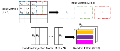
Let us assume that a input is convoluted with kernels in each channel. Since the kernel size is , the input vectors extracted from the input matrix are of size as shown in Figure 7(a). Since each input vector has elements, the random projection matrix, , is of size for . We can re-organize each column vector of into the shape . With this organization, we can treat each column vector of (i.e., to ) as a random filter of size .

Let us consider an input vector . converts into a signature consisting of bits (i.e., to ) using RPQ algorithm (II-A). is calculated by performing a dot product between and followed by a sign comparison. Other bits, to , are calculated similarly. Similarly, can be calculated from and so on. In other words, if we perform a 2D convolution followed by a sign comparison by sliding over all input vectors from , we can calculate the first bit of each signature (i.e., , , , ). Similarly, the convolution between and the input vectors will produce the second bit of each signature and so on. In other words, the signature calculation can be formulated as convolutions between input vectors and random filters to . Therefore, we can easily map it to a row-stationary accelerator.
Assume that the accelerator has PEs. Figure 7(b) shows the signature calculation process. Mercury starts with the random filter and computes convolutions with each input vector. Filter rows stream horizontally while input rows stream diagonally. So to perform 3(three) 2D convolutions in a streaming fashion - , , and then, . indicates a 2D convolution. We refer to the set of PEs working on a 2D convolution as a PE Set. Thus, consists of to . With streaming first, calculates , and then, . After that, is loaded, and the second bit of each signature is calculated. Thus, bits of all signatures are calculated through convolutions with random filters.
III-B2 Dataflow of Signature Calculation
Let us continue with our example in III-B1. to are the elements of and to are the elements of . Figure 8(a) shows the timing of signature calculation in a row-stationary accelerator. With input vectors, it takes four cycles to multiply and accumulate the result of each row and two cycles to accumulate across rows. Thus, it takes six cycles to generate a single bit of a signature. Similarly, the first bit of subsequent signatures takes six cycles each. In general, for input vectors, it takes cycles to calculate each bit of a signature. However, the calculation of one bit of one signature does not overlap with that of another signature (as shown in Figure 8(c)(a)). Note that we do not assume a separate multiplier and adder unit in each PE. Instead, if we assume a multiply-accumulate (MAC) unit, it takes cycles to calculate a single bit of a signature (because row accumulation takes one less cycle). However, still, each signature is calculated in a non-overlapping fashion.

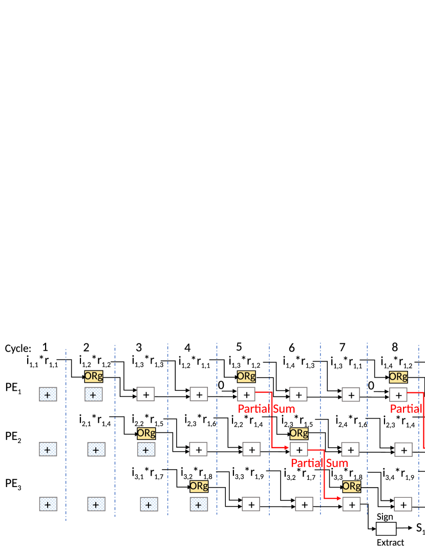

We propose to pipeline the calculation of one signature with another. The core idea is to add a register, named Overlapped register (ORg), in each PE and intentionally delay the calculation starting time of and by 1 and 2 cycles, respectively (as shown in Figure 8(b)). This is reminiscent of software pipelining [51]. ORg register is used to hold the result of multiplying the first element of each row of input and random vectors. For example, ORg of is used to hold in cycle 2 and in cycle 5. When the register holds in cycle 5, it frees up the adder unit which can be used to pass the row accumulation result from to in cycle 6. Similarly in cycle 6, ORg of holds which frees up the adder. Therefore, the adder accumulates the result from with and passes it to in cycle 7. In cycle 7, ORg of holds which frees up the adder to finish the accumulation of all rows. Thus, takes seven cycles to calculate. However, the calculation of has already started. Therefore, following the same flow, will finish in cycle 10, i.e., it takes only three more cycles. Similarly, the first bit of subsequent signatures produced by the same PEs will take 3 more cycles each. Generally, for input vectors, the first bit of the first signature calculated by a set of PEs takes cycles, while other bits of any signature take cycles to finish. This is illustrated in Figure 8(c)(b).
III-B3 Signature Management
Mercury manages signatures using three structures - Signature Table, MCache, and Hitmap. The Signature Table stores the signatures, MCache keeps dot product results computed between different input and weight vectors, and the Hitmap keeps track of which signature causes a hit in MCache. The Signature Table is indexed by the input vector number so that Mercury can easily find it for a particular input vector. When a signature is calculated by the PEs, Mercury stores it in the signature table and then accesses MCache. MCache is indexed and tagged with the signature. MCache keeps computed dot product results so that input vectors with similar signature can reuse them. The data portion of MCache contains the results. MCache differs from a normal cache in two ways. First, since a tag (i.e., signature) is produced before the data (i.e., computed results), cache tag and data are not updated together. To accommodate that, each cache line has two valid bits - Valid Tag (VT) and Valid Data (VD). When a signature is used to initialize the tag section of a cache line, its VT is set while VD remains unset. The data portion of MCache is populated and used as a weight vector (or derivative) is multiplied with the input vector. Different weight vectors populate the data portion with different results (details in III-C). Second, there is no replacement in MCache. When a set is full, no new entries are inserted into MCache. We choose this no replacement policy approach to simplify the design of MCache.

Figure 9 shows what happens when a signature, for a new input vector is calculated. If is already in MCache, we have a hit. So, the Hitmap entry is set to HIT. Otherwise, is a new signature; therefore, MCache checks if the corresponding set is full. If it is not full, is inserted into the cache by updating the tag portion of an entry. Since the data portion will be updated later, the Hitmap entry is marked as Miss And Update (MAU). If the set is full, will not be inserted into MCache. Since no cache entry will be updated, the Hitmap entry is marked as Miss No Update (MNU). When a new set of input vectors are extracted from an input matrix, MCache, Signature table, and Hitmap are cleared.
III-C Exploiting Input Similarity
Here, we explain how signatures along with MCache can be utilized to skip similar computations in the forward propagation followed by the backward propagation. We will first explain it for a convolution layer ( III-C1 & III-C2). In III-C3 and III-C4, we will address it for other layers.
III-C1 Computation Reuse in Forward Propagation
During the forward propagation of a convolution layer, a input convolves with a number of filters in a channel. The input consists of a number of input vectors, each with the same size as a filter. Thus, for each channel, an accelerator performs a number of dot products between the input vectors and filters in that channel. The PEs load one filter and a number of input vectors at a time and perform the dot products. The input vectors and filters are passed through the PEs in a streaming fashion. Rows of input vectors are passed through diagonally, whereas rows of filters are passed through horizontally. Partial sums are accumulated vertically. Figure 10 shows this flow. Here, we assume that , , and perform a dot product between an input vector and a filter. Thus, PE Set 1 consists of to . Similarly, PE Set 2 consists of to .

Each PE has an input buffer, a number of input and weight registers, a multiplier, and an adder. The input buffer holds inputs as they arrive at the PE. Input registers load values from the input buffer. As filter weights arrive, they are stored in the weight registers. The multiplier and adder work with the values from the input and weight registers. Each PE in PE set starts with the first input vector from its input buffer. Each PE checks whether the corresponding entry in the Hitmap is a HIT. Remember that the Hitmap and signatures are calculated before the convolution operations for a channel begin. A HIT indicates that the input vector is similar to an earlier one; hence, the dot product result stored in the MCache can be reused instead of calculating again. That is why the PE skips the dot product. Instead, using the signature of the input vector, the stored result is fetched from MCache and used as the PE set result. On the other hand, if the entry in the Hitmap is MAU or MNU, the PEs in the PE set perform the dot product. If the Hitmap entry is MAU, the corresponding MCache line contains the signature of this input vector, but the result (data) portion is still empty. So, the data portion is updated with the dot product result, and its VD is set. If the Hitmap entry is MNU, MCache does not contain the signature at all. So, Mercury does not store the dot product result in the cache. The PEs in the PE set proceed with the next input vector from the respective input buffer. Note that although a PE set might skip computations occasionally, the dataflow (filter streaming horizontally and inputs streaming diagonally) remains unchanged due to the Hitmap.
If we assume the same inputs as in III-B1, then operates on input vectors , , and whereas operates on input vectors , , and in Figure 10. Therefore, at first, the PEs in check entry of the hitmap. Based on that entry, the PEs either reuse results from MCache or compute dot products using input vector and the current filter. For the example in Figure 10, will compute dot product because entry is MAU. On the other hand, the PEs in check entry in the hitmap and act accordingly. Note that each PE set acts independent of other PE sets. As a result, one PE set might reuse a lot of computed results and finish computations early whereas another PE set may lag behind computing many dot products. We propose two designs to address this - synchronous and asynchronous.
- Synchronous Design: In synchronous design, when a PE set finishes computation, it waits until all other PE sets are done. Each PE set maintains a busy bit (B). A controller checks all B bits. If none of them are busy (i.e., ), the controller instructs the PEs to load with the next filter and input vectors. At this point, MCache may contain computed results from the previous filter and input vectors. Those results cannot be used because weights change in the new filter. Therefore, MCache invalidates all VD bits. A bitline connecting all VD bits is used for this purpose. The input vectors remain the same within the same channel. Therefore, VT flags and Hitmap are still valid and kept as they are. When Mercury proceeds with the next channel, the signatures in the signature table, MCache, and Hitmap are recalculated and reinitialized.
- Asynchronous Design: The synchronous design is intuitive and simpler but limits performance improvement because the faster PE sets remain idle until the slowest one completes. Therefore, we propose an asynchronous design where the faster PE sets can work on the next filter and input vectors while the slower ones work on the previous filter and input vectors. However, this requires additional buffer and co-ordination scheme.

Figure 11 shows the changes required for the asynchronous design. There are major changes. First, to store new input vectors each PE is extended to have two input buffers. Each buffer has an associated valid (V) bit to indicate whether it contains valid inputs or not. Moreover, each PE has a register, named InUse, to indicate which of the two buffers is currently used. All PEs in a PE set will have the same value in the InUse register. With the extra buffer, whenever the fastest PE set completes computation, it loads next input vectors in streaming fashion as before. PEs in other PE sets store the new input vectors in the unused input buffer. That way, when those PE sets finish computations, new input vectors are already available in one of the input buffers. Second, the accelerator stores multiple filters in a shared buffer so that each PE can access it. Each filter has an associated BusyMap to indicate which PE sets are currently busy with that filter. Each PE maintains a register, named FlUse, to indicate which filter it is using. Like InUse, the FlUse register has the same value in each PE of a PE set. When all PE sets finish using a filter, it is loaded with a new filter and the BusyMap is initialized. Third, since each input vector and filter produces a new dot product result, we propose to make MCache a multi-version cache where each cache line has multiple versions of data. Each data portion has a VD bit to indicate whether it is valid or not. Note that there are as many versions as the number of filters. Thus, if a PE set tries to use a new filter when there is no space to store it (because all M filters are marked busy with at least one PE set), then the PEs in the PE set will remain idle until a filter is completely used up in all PE sets. When the PEs in a PE set access a cacheline, they use FlUse register to determine which data version should be used.
III-C2 Input Similarity in Backward Propagation
There are two major computations - (i) calculation of weight derivatives () of the current layer (say, layer ), and (ii) calculation of output derivatives of the previous layer (). Here, boldfaced letters indicate multidimensional tensors. Now, let us consider the computation of . We observe that is the same as . Therefore, if the filters of layer have the same dimension as those of layer , the signatures and Hitmap produced by layer for can be applied to to find similarity. In that case, this computation scenario is the same as the forward propagation computation of layer . Based on this observation, we propose saving signatures and the Hitmap of each layer during the forward propagation and reloading them during the previous layer’s backward propagation. Then, Mercury applies the same technique as in III-C1. However, if the filter’s dimensions do not match, Mercury recalculates the signatures of gradient vectors and repopulates the Hitmap to reuse computations.

III-C3 Input Similarity in a Fully Connected Layer
Figure 12 shows the high-level computations for a minibatch (size ) of inputs. Inputs and weights are divided into blocks based on the number of PEs. Suppose there are two input blocks and two weight blocks. One PE multiplies Input of block with of weight block 1 followed by , , … . Concurrently another PE multiplies Input and followed by to . This continues up to Input . Thus, if one input is similar to another, the earlier one’s multiplication with () can be reused for the later one. Before the multiplication with weights begins, signatures and Hitmap are initialized based on the inputs of block 1 as in III-B. Before a PE multiplies an input vector (e.g., Input ) with a weight vector (e.g., ), the Hitmap of that input is checked. Depending on a HIT, MAU, or MNU, the result is either reused or calculated. This is similar to that of a convolution layer ( III-C1). In the case of a HIT, we store the id of the newly matched signature in the PE (that is processing the input corresponding to the stored signature causing the match). Let us refer to this PE as the earlier PE. During the multiplication with weights, whenever the result for one weight gets ready, the earlier PE sends the result to later PEs (that are processing the inputs of the matched signatures) one by one to update their output. Sending results to other PEs is done in parallel with the regular operation. The earlier PE will start the operation of the next weight immediately after finishing with the current weight. In case the earlier PE is done with the next weight before the result is sent to all of the matched signature-related PEs, the earlier PE is stalled until the send operations finish. The earlier PE (after finishing block input) loads an input from block and starts signature generation while other PEs keep processing inputs and weights from block . For doing this, we break the MCache into two separate caches, and PEs in each block will write and update the associated cache. The earlier PE can start multiplication with weights immediately after the signature generation process since the required results from block have already been computed and sent to the PEs that need it. Race can arise when one PE wants to write to its related output memory while the earlier PE’s results are ready, and it needs to write them into memory output too. We designed a simple conflict handler for handling these simultaneous write requests. Once all the inputs from block 1 is multiplied by the weights from block 1, PEs can start the operation of block 2 of inputs. Similar to block 1, they will start with signature generation and Hitmap initialization. Some PEs may have already started the operation of block 2 inputs, and their signatures are in the related MCache part, and new PEs can get results from these PEs in case of a signature match.
III-C4 Input Similarity in an Attention Layer
An attention layer is used in a sequence-to-sequence model [58]. Let’s assume that the input vectors are and the output vectors are . For simplicity, assume both and to have the same sequence length (i.e., ) and the same vector representation of length . To produce output vector , the attention layer simply takes a weighted average over all input vectors, . Here is not parametric but rather a weighted matrix representing the correlation between each element of . can be calculated as . We can calculate . Here is simply a matrix-matrix multiplication. Thus, we can apply our idea of input similarity to calculate by exploiting the similarity among vectors. Because this computation is similar to a fully connected layer, we apply the same technique as in III-C3.
III-D Adaptation in Mercury
As training proceeds, DNN models become more sensitive to computation reuse. So, we propose Mercury to be adaptive.
Increase in Signature Length: If signature length increases, vectors and are found to have similarity only when becomes significantly smaller. So, a larger signature has a lesser effect on model accuracy but it may reduce computation reuse. Therefore, Mercury starts with a smaller signature size (e.g., 20 bits long) and progressively increases signature length as the model is trained more. Towards this end, Mercury calculates the average loss in each iteration during training. If there is no change in the loss for consecutive iterations, then Mercury increments signature length by 1.
Stoppage of Similarity Detection: Mercury analytically determines if detecting similarity can save computations or not. If no computation can be saved, then Mercury turns off the similarity detection phase. In order to implement this, Mercury records the total computation cost (i.e., cycles) for signature generation in forward and backward propagation when some computations are reused. This cost is compared with the total computation cost of the baseline system without any computation reuse. can be calculated analytically using different hardware components’ latency. If the former cost is more than the later for consecutive batches of inputs, Mercury stops generating signatures.
IV Support for different dataflows
Mercury can be easily implemented in other dataflow accelerators. Here we explain it for weight and input stationary dataflows.
Weight-Stationary Dataflow: Weights are stationary in the PEs, and input vectors are broadcasted to PEs. Mercury keeps the original dataflow structure the same and loads random vectors as the first part of filters. So, random vectors will initially be loaded to different PEs, and one input vector will be broadcasted to PEs. The signatures are generated using the original Weight-Stationary dataflow. However, after loading random vectors, one input vector’s signature will be stored in several PEs, and several PEs will update the signature table for different vectors. Then, using the generated signature table and the proposed MCache structure, Mercury will detect similarity using signatures and specify the hit/miss for them. The next step is loading the regular filters, but Mercury already knows which input vectors are similar. So, while reading vectors from global memory, Mercury skips similar vectors and reuses the results.
Input-Stationary Dataflow: Inputs are stationary in PEs, and weights will be broadcasted. The hardware first finishes the operation of one input vector before loading a new input vector. The global structure of Mercury in Input-Stationary dataflow is similar to Weight-Stationary dataflow, which loads random vectors as the first part of filters. So, one input vector will be loaded to different PEs, random vectors will be loaded to different PEs at the beginning, and weight matrices will be streamed into PEs. The signatures are generated using the original Input-Stationary dataflow and the Hitmap is initialized accordingly. During actual operation, if there is a hit for an input vector, MCache skips the rest of the weights and loads the next input vector. However, Mercury will continue streaming the weights if there is a miss for current input.
V Implementation Details
MCache Design: To make MCache scalable, we make two design decisions. First, MCache is implemented in shared memory using slice registers (flip flops in FPGA) that can be accessed through id. Multiple PE sets can read the same cache entry within a fixed delay using the id. That is why, the entry id is saved along with the signature in the signature table. Since an inserted signature is not removed from the cache until a new channel starts, further accesses to that signature are done through the id without requiring comparison. Second, we add a queue and a simple controller for each cache set. Thus, a cache set can be updated independently. To insert multiple signatures simultaneously into a cache set, the queue records the requests, and the controller serializes them - one at a time. Multiple signature insertions for different cache sets can proceed simultaneously without any issue. Although these techniques are specifically for FPGA, for an ASIC accelerator, similar techniques such as banked cache [30], multi-signature cache line, and PE set wise smaller cache can be used. We leave the details of ASIC design for future.
PE Implementation: The structure of PE in Mercury is similar to a typical PE [10] as shown in Figure 11. Each PE has an extra block memory to store one input row. The original Row Stationary dataflow needs enough input buffers to store one row of one vector in each PE. This is implemented using Slice Registers which are limited in FPGA. In PE implementation, we reduce the input buffer to only one register and use the local block memory to process the inputs and store the results back. For Synchronous design, since all PEs are in the same phase at a time, one extra block memory is enough. However, since the first and second phases can be done by different PE sets independently in Asynchronous design, we implement multiple filters using block memory. Table I shows the types of memories used in the implementation of Mercury .
| Memory Type | Mercury Components |
|---|---|
| Block Memory | Global Buffer, Input Buffer, Signature Table |
| Slice Register | MCache, Filters, Hitmap, Input/Weight registers, |
| InUse/FIUse flags, ORg |
VI Experimental Setup
The hardware implementation of Mercury is done on a Virtex 7 FPGA board [59] configured using the Xilinx Vivado [60] software. We used an Eyeriss-style [10] row stationary accelerator with the same number of PEs (i.e., 168) as the baseline. The model’s inputs and weights are stored in an external SSD connected to the FPGA. We use 1024 entries and associativity of 16 for MCache. VII-C analyzes the performance impact of different MCache organizations. All performance, power consumption, hardware utilization, and other hardware-related metrics are collected from the synthesized FPGA design using Vivado. Different model accuracy results are collected from PyTorch [48] implementation. We consider 12 networks: AlexNet, GoogleNet, VGG13, VGG16, VGG19, ResNet50, ResNet101, ResNet152, Inception-V4, MobileNet-V2, SqueezeNet-1-0, and Transformer. We use 80 image classes from ImageNet and report top 1% accuracy for CNN models. For transformer, we use Multi30k dataset and report accuracy and Bleu score. We train the models until the highest reported accuracy is reached in the baseline system. For Mercury, we trained the models with the same number of epochs. VII-D provides a comparison with UCNN [29], Unlimited Zero-Pruning, and Unlimited Similarity Detection.
VII Evaluation
VII-A Accuracy and Performance Comparision
Figure 13 shows the impact of Mercury on the models’ accuracy. Overall, there is a reduction in validation accuracy111Hyper-parameters are adjusted in training to achieve optimal accuracy. Considering the inherent randomness during the training process, we argue that Mercury’s accuracy is comparable to the baseline system. Also, we got the same bleu_score of on test data for the transformer.

Figure 14(a) shows the adaptivity of Mercury across different models. Based on the similarity detection costs in layers and the overall performance during the model training, Mercury may turn off similarity detection in some layers during the training. Figure 14(b) shows the computational cycle breakdown of Mercury and baseline. This cycles includes computation cycles of convolutional, fully connected, and attention layers as well as signature calculation. Most of the cycles belong to the layer computations. The signature computation accounts for only a fraction of the total cycles. Overall, Mercury can reduce the total computation time by about , which results in an average speedup of , as shown in Figure 14(c). For bigger networks, such as ResNet152, VGG19, and Inception-V4, there are more saving opportunities since there are more chances of similarity between vectors.


VII-B Case Study: VGG13
We conduct a detailed analysis of VGG13 to show how Mercury works at runtime, focusing on the characterization of the MCache access, the savings, and the number of unique vectors found across layers. The results are shown in Figure 15. Figure 15(a) shows a gradual increase in MCache Hit and MAU percentage due to the reduction in the number of input vectors and cache occupants. Figure 15(b) shows that the computational cycles may vary across layers of VGG13 due to the difference in layers’ size and channels. Some layers have a higher cycle count related to the input size and number of input and output channels, and the amount of savings differs. The number of unique vectors is also different across layers. As shown in Figure 15(c), the first few layers have the highest number of unique vectors since they have a large input size. This value is lower for the later layers due to the smaller input size.


VII-C Performance Impact of Different Organizations of MCache
This section analyzes the impact of different MCache sizes and organizations on the performance of Mercury. As shown in Figure 16, Mercury performance increases with cache size and associativity. Unfortunately, Vivado did not finish synthesis of 32-way cache-based designs even after one day (our time limit for the server). Thus, we had to limit ourselves to 8 or 16-way. Combining with Table IV shows that moving from a 512-entry, 8-way to a 1024-entry, 16-way cache only increases the power consumption by while giving more speed up. Doubling the cache size to entries gives insignificant performance gains; thus, -entry and -way is selected as the default configuration for MCache.


VII-D Comparative Analysis


VII-D1 Comparison with UCNN in inference mode
To compare with UCNN during inference, we perform the following scenario. First, we compute the static quantization for all layers of the pretrained model with a different number of bits. We only considered 6 to 8-bit quantizations since there was a significant loss in accuracy beyond this point. With 6-bits quantization, the final accuracy drops about . Second, based on [29], we need to find similar items in one filter, do the activation group reuse, and then save all the additions with totally or partially similar activation groups. Due to the lack of access to the implementation of [29], we considered the maximum saving in each filter. In other words, in an activation group reuse with length k, suppose we have similar indices in other filters, and we can save additions between all members. Figure 17(a) shows a comparison between Mercury and the maximum achievable speedup of UCNN with different quantization policies. On average, Mercury outperforms UCNN with 7 and 8-bit quantization while achieving comparable performance gains to the 6-bit quantization version.
VII-D2 Comparison with Unlimited Zero Pruning
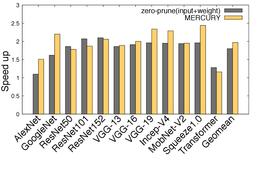
Here, we compare Mercury against the theoretical upper bound of Zero-Pruning, which assumes the accelerator can detect and save all zero-related computations in both input and weights. Figure 17(b) shows the comparison between Mercury versus the theoretical maximum achievable speedup of Zero Pruning. On average, Mercury outperforms by 4%. Note that in actual hardware, the performance gains of Zero Pruning will be limited by hardware resource constraints and zero-value detection and bypass overhead.
VII-D3 Comparison with Unlimited Similarity Detection
This scenario finds and saves all similar elements in a model’s inputs and weights. Similar to the Zero Pruning scenario, we did not consider any limitations on the amount of similarity. We assumed that the accelerator could find and save the computation of all similar elements. Figure 17(c) shows the speedup of Mercury versus the Unlimited Similarity Detection scheme. On average, our approach performs better than the Unlimited Similarity technique.
VII-E Results with Other Dataflows
Figure 18(a) and 18(b) show the speedup of our scheme when deployed on top of the Input-Stationary and Weight-Stationary dataflow. For Input-Stationary, Mercury gives an average performance gains of over the baseline. The maximum speedup of is achieved in VGG-19. Mercury works better with Weight-Stationary as it achieves an average speedup of over the baseline. The maximum speedup of is observed in ResNet101.


VII-F Hardware Utilization Analysis
| Cache | # | #Slice | #Slice | #Block | |
|---|---|---|---|---|---|
| Size | Sets | LUTs | Registers | RAM | #DSP48E1s |
| 256 | 16 | 140597 | 62620 | 1177.5 | 198 |
| 512 | 32 | 211437 | 69536 | 1193.5 | 198 |
| 768 | 48 | 216544 | 74925 | 1209.5 | 198 |
| 1024 | 64 | 216918 | 81332 | 1225.5 | 198 |
(a) Resource usage
| # | Block | ||||||
|---|---|---|---|---|---|---|---|
| Sets | Clocks | Logic | Signals | RAM | DSPs | Static | Total |
| 16 | 0.138 | 0.102 | 0.18 | 0.516 | 0.087 | 0.681 | 1.811 |
| 32 | 0.154 | 0.104 | 0.175 | 0.524 | 0.087 | 0.683 | 1.833 |
| 48 | 0.155 | 0.103 | 0.201 | 0.548 | 0.087 | 0.685 | 1.884 |
| 64 | 0.166 | 0.105 | 0.216 | 0.561 | 0.087 | 0.687 | 1.929 |
(b) On-chip power consumption (watt)
| Cache | #Slice | #Slice | #Block | ||
|---|---|---|---|---|---|
| Size | #Ways | LUTs | Registers | RAM | #DSP48E1s |
| 128 | 2 | 216777 | 65727 | 1225.5 | 198 |
| 256 | 4 | 216618 | 67897 | 1225.5 | 198 |
| 512 | 8 | 216758 | 71999 | 1225.5 | 198 |
| 1024 | 16 | 216918 | 81332 | 1225.5 | 198 |
(a) Resource usage
| # | Block | ||||||
|---|---|---|---|---|---|---|---|
| Ways | Clocks | Logic | Signals | RAM | DSPs | Static | Total |
| 2 | 0.146 | 0.1 | 0.176 | 0.555 | 0.087 | 0.686 | 1.855 |
| 4 | 0.151 | 0.104 | 0.197 | 0.543 | 0.087 | 0.686 | 1.874 |
| 8 | 0.157 | 0.101 | 0.18 | 0.559 | 0.087 | 0.686 | 1.876 |
| 16 | 0.166 | 0.105 | 0.216 | 0.561 | 0.087 | 0.687 | 1.929 |
(b) On-chip power consumption (watt)
| #Slice | #Slice | #Block | ||
|---|---|---|---|---|
| Method | LUTs | Registers | RAM | #DSP48E1s |
| Baseline | 56910 | 48735 | 1161.5 | 198 |
| Mercury | 216918 | 81332 | 1225.5 | 198 |
(a) Resource usage
| Block | |||||||
|---|---|---|---|---|---|---|---|
| Method | Clocks | Logic | Signals | RAM | DSPs | Static | Total |
| Baseline | 0.112 | 0.07 | 0.138 | 0.511 | 0.087 | 0.678 | 1.703 |
| Mercury | 0.166 | 0.105 | 0.216 | 0.561 | 0.087 | 0.687 | 1.929 |
(b) On-chip power consumption (watt)
In this section, we provide a detailed analysis of the resource usage and power consumption of Mercury implementation on the Virtex 7 FPGA board. Table IV compares the resource usage and on-chip power consumption of Mercury for different MCache sizes. Specifically, quadrupling the number of MCache sets only increases the overall power consumption by . If we fix the number of sets to and increase the number of ways from to , the power consumption increases by , as shown in Table IV. This result indicates that Mercury design can work with different sizes of cache and various number of ways with reasonable overhead. As shown in Table IV, Mercury increases resource usage and the power consumption by . The majority of this increment is related to the power of Signals and Logic which is the result of using adaptable cache-based structure in the proposed design. However, as explained in V, since we fixed the cache size and number of ways to an optimal value, the Mercury resource consumption will be almost the same even if we increase the size of input images and number of PEs.
VIII Conclusions
We proposed a novel scheme based on RPQ to exploit the similarity of computations during DNN training in a hardware accelerator. The proposed scheme, called Mercury, uses a cache (MCache) to store signatures of recent input vectors along with the computed results. If a new input vector’s signature matches with an existing signature in the MCache, the already-computed result is reused for the new vector. Mercury is the first work that exploits computational similarity using RPQ for accelerating DNN training in hardware. We present a detailed design, workflow, and implementation of Mercuryfor multiple layers and dataflows. This work opens up a new direction for speeding up hardware accelerators by optimizing computations for the deep learning process. Our experimental evaluation with twelve different deep learning models shows that Mercury speeds up the training by with an accuracy similar to the baseline system.
References
- [1] V. Akhlaghi, A. Yazdanbakhsh, K. Samadi, R. K. Gupta, and H. Esmaeilzadeh, “Snapea: Predictive early activation for reducing computation in deep convolutional neural networks,” in 2018 ACM/IEEE 45th Annual International Symposium on Computer Architecture (ISCA), 2018, pp. 662–673.
- [2] J. Albericio, P. Judd, T. Hetherington, T. Aamodt, N. E. Jerger, and A. Moshovos, “Cnvlutin: Ineffectual-neuron-free deep neural network computing,” in 2016 ACM/IEEE 43rd Annual International Symposium on Computer Architecture (ISCA), 2016, pp. 1–13.
- [3] M. Alwani, H. Chen, M. Ferdman, and P. Milder, “Fused-layer cnn accelerators,” in 2016 49th Annual IEEE/ACM International Symposium on Microarchitecture (MICRO), 2016, pp. 1–12.
- [4] Y. Bengio, Y. LeCun et al., “Scaling learning algorithms towards ai,” Large-scale kernel machines, vol. 34, no. 5, pp. 1–41, 2007.
- [5] E. Bingham and H. Mannila, “Random projection in dimensionality reduction: Applications to image and text data,” in Proceedings of the Seventh ACM SIGKDD International Conference on Knowledge Discovery and Data Mining, ser. KDD ’01. New York, NY, USA: Association for Computing Machinery, 2001, p. 245–250. [Online]. Available: https://doi.org/10.1145/502512.502546
- [6] B. H. Bloom, “Space/time trade-offs in hash coding with allowable errors,” Communications of the ACM, vol. 13, no. 7, pp. 422–426, 1970.
- [7] L. Ceze, J. Tuck, J. Torrellas, and C. Cascaval, “Bulk disambiguation of speculative threads in multiprocessors,” in Proceedings of the 33rd Annual International Symposium on Computer Architecture, ser. ISCA ’06. USA: IEEE Computer Society, 2006, p. 227–238. [Online]. Available: https://doi.org/10.1109/ISCA.2006.13
- [8] M. S. Charikar, “Similarity estimation techniques from rounding algorithms,” in Proceedings of the Thiry-Fourth Annual ACM Symposium on Theory of Computing, ser. STOC ’02. New York, NY, USA: Association for Computing Machinery, 2002, p. 380–388. [Online]. Available: https://doi.org/10.1145/509907.509965
- [9] T. Chen, Z. Du, N. Sun, J. Wang, C. Wu, Y. Chen, and O. Temam, “Diannao: A small-footprint high-throughput accelerator for ubiquitous machine-learning,” ser. ASPLOS ’14. New York, NY, USA: Association for Computing Machinery, 2014, p. 269–284. [Online]. Available: https://doi.org/10.1145/2541940.2541967
- [10] Y. Chen, J. Emer, and V. Sze, “Eyeriss: A spatial architecture for energy-efficient dataflow for convolutional neural networks,” in 2016 ACM/IEEE 43rd Annual International Symposium on Computer Architecture (ISCA), 2016, pp. 367–379.
- [11] Y. Chen, J. Emer, and V. Sze, “Using dataflow to optimize energy efficiency of deep neural network accelerators,” IEEE Micro, vol. 37, no. 3, pp. 12–21, 2017.
- [12] Y. Chen, T. Luo, S. Liu, S. Zhang, L. He, J. Wang, L. Li, T. Chen, Z. Xu, N. Sun, and O. Temam, “Dadiannao: A machine-learning supercomputer,” in 2014 47th Annual IEEE/ACM International Symposium on Microarchitecture, 2014, pp. 609–622.
- [13] P. Chi, S. Li, C. Xu, T. Zhang, J. Zhao, Y. Liu, Y. Wang, and Y. Xie, “Prime: A novel processing-in-memory architecture for neural network computation in reram-based main memory,” in 2016 ACM/IEEE 43rd Annual International Symposium on Computer Architecture (ISCA), 2016, pp. 27–39.
- [14] N. M. Cicek, L. Ning, O. Ozturk, and X. Shen, “General reuse-centric cnn accelerator,” IEEE Transactions on Computers, pp. 1–1, 2021.
- [15] N. M. Cicek, X. Shen, and O. Ozturk, “Energy efficient boosting of gemm accelerators for dnn via reuse,” ACM Trans. Des. Autom. Electron. Syst., dec 2021, just Accepted. [Online]. Available: https://doi.org/10.1145/3503469
- [16] C. Coleman, C. Yeh, S. Mussmann, B. Mirzasoleiman, P. Bailis, P. Liang, J. Leskovec, and M. Zaharia, “Selection via proxy: Efficient data selection for deep learning,” arXiv preprint arXiv:1906.11829, 2019.
- [17] M. Courbariaux and Y. Bengio, “Binarynet: Training deep neural networks with weights and activations constrained to +1 or -1,” in Conference on Neural Information Processing Systems (NIPS), 2016.
- [18] D. Das, N. Mellempudi, D. Mudigere, D. Kalamkar, S. Avancha, K. Banerjee, S. Sridharan, K. Vaidyanathan, B. Kaul, E. Georganas, A. Heinecke, P. Dubey, J. Corbal, N. Shustrov, R. Dubtsov, E. Fomenko, and V. Pirogov, “Mixed precision training of convolutional neural networks using integer operations,” in International Conference on Learning Representations (ICLR), 2018.
- [19] J. Dean, G. Corrado, R. Monga, K. Chen, M. Devin, M. Mao, M. a. Ranzato, A. Senior, P. Tucker, K. Yang, Q. Le, and A. Ng, “Large scale distributed deep networks,” in Advances in Neural Information Processing Systems, F. Pereira, C. Burges, L. Bottou, and K. Weinberger, Eds., vol. 25. Curran Associates, Inc., 2012. [Online]. Available: https://proceedings.neurips.cc/paper/2012/file/6aca97005c68f1206823815f66102863-Paper.pdf
- [20] A. Delmas Lascorz, P. Judd, D. M. Stuart, Z. Poulos, M. Mahmoud, S. Sharify, M. Nikolic, K. Siu, and A. Moshovos, “Bit-tactical: A software/hardware approach to exploiting value and bit sparsity in neural networks,” ser. ASPLOS ’19. New York, NY, USA: Association for Computing Machinery, 2019, p. 749–763. [Online]. Available: https://doi.org/10.1145/3297858.3304041
- [21] Z. Du, R. Fasthuber, T. Chen, P. Ienne, L. Li, T. Luo, X. Feng, Y. Chen, and O. Temam, “Shidiannao: Shifting vision processing closer to the sensor,” in 2015 ACM/IEEE 42nd Annual International Symposium on Computer Architecture (ISCA), 2015, pp. 92–104.
- [22] R. D. Evans, L. Liu, and T. M. Aamodt, “Jpeg-act: Accelerating deep learning via transform-based lossy compression,” in Proceedings of the ACM/IEEE 47th Annual International Symposium on Computer Architecture, ser. ISCA ’20. IEEE Press, 2020, p. 860–873. [Online]. Available: https://doi.org/10.1109/ISCA45697.2020.00075
- [23] D. Feldman, Core-Sets: Updated Survey. Cham: Springer International Publishing, 2020, pp. 23–44. [Online]. Available: https://doi.org/10.1007/978-3-030-29349-9_2
- [24] Y. Freund, S. Dasgupta, M. Kabra, and N. Verma, “Learning the structure of manifolds using random projections,” in Advances in Neural Information Processing Systems, J. Platt, D. Koller, Y. Singer, and S. Roweis, Eds., vol. 20. Curran Associates, Inc., 2007. [Online]. Available: https://proceedings.neurips.cc/paper/2007/file/9fc3d7152ba9336a670e36d0ed79bc43-Paper.pdf
- [25] A. Gondimalla, N. Chesnut, M. Thottethodi, and T. N. Vijaykumar, “Sparten: A sparse tensor accelerator for convolutional neural networks,” in Proceedings of the 52nd Annual IEEE/ACM International Symposium on Microarchitecture, ser. MICRO ’52. New York, NY, USA: Association for Computing Machinery, 2019, p. 151–165. [Online]. Available: https://doi.org/10.1145/3352460.3358291
- [26] J. Gu, Z. Wang, J. Kuen, L. Ma, A. Shahroudy, B. Shuai, T. Liu, X. Wang, G. Wang, J. Cai, and T. Chen, “Recent advances in convolutional neural networks,” Pattern Recogn., vol. 77, no. C, p. 354–377, May 2018. [Online]. Available: https://doi.org/10.1016/j.patcog.2017.10.013
- [27] S. Han, H. Mao, and W. Dally, “Deep compression: Compressing deep neural networks with pruning, trained quantization and huffman coding,” in International Conference on Learning Representations (ICLR), 2016.
- [28] S. Han, X. Liu, H. Mao, J. Pu, A. Pedram, M. A. Horowitz, and W. J. Dally, “Eie: Efficient inference engine on compressed deep neural network,” in 2016 ACM/IEEE 43rd Annual International Symposium on Computer Architecture (ISCA), 2016, pp. 243–254.
- [29] K. Hegde, J. Yu, R. Agrawal, M. Yan, M. Pellauer, and C. Fletcher, “Ucnn: Exploiting computational reuse in deep neural networks via weight repetition,” in 2018 ACM/IEEE 45th Annual International Symposium on Computer Architecture (ISCA), 2018, pp. 674–687.
- [30] J. L. Hennessy and D. A. Patterson, Computer Architecture, Fifth Edition: A Quantitative Approach, 5th ed. San Francisco, CA, USA: Morgan Kaufmann Publishers Inc., 2011.
- [31] A. Jain, A. Phanishayee, J. Mars, L. Tang, and G. Pekhimenko, “Gist: Efficient data encoding for deep neural network training,” in Proceedings of the 45th Annual International Symposium on Computer Architecture, ser. ISCA ’18. IEEE Press, 2018, p. 776–789. [Online]. Available: https://doi.org/10.1109/ISCA.2018.00070
- [32] N. P. Jouppi, C. Young, N. Patil, D. Patterson, G. Agrawal, R. Bajwa, S. Bates, S. Bhatia, N. Boden, A. Borchers, R. Boyle, P.-l. Cantin, C. Chao, C. Clark, J. Coriell, M. Daley, M. Dau, J. Dean, B. Gelb, T. V. Ghaemmaghami, R. Gottipati, W. Gulland, R. Hagmann, C. R. Ho, D. Hogberg, J. Hu, R. Hundt, D. Hurt, J. Ibarz, A. Jaffey, A. Jaworski, A. Kaplan, H. Khaitan, D. Killebrew, A. Koch, N. Kumar, S. Lacy, J. Laudon, J. Law, D. Le, C. Leary, Z. Liu, K. Lucke, A. Lundin, G. MacKean, A. Maggiore, M. Mahony, K. Miller, R. Nagarajan, R. Narayanaswami, R. Ni, K. Nix, T. Norrie, M. Omernick, N. Penukonda, A. Phelps, J. Ross, M. Ross, A. Salek, E. Samadiani, C. Severn, G. Sizikov, M. Snelham, J. Souter, D. Steinberg, A. Swing, M. Tan, G. Thorson, B. Tian, H. Toma, E. Tuttle, V. Vasudevan, R. Walter, W. Wang, E. Wilcox, and D. H. Yoon, “In-datacenter performance analysis of a tensor processing unit,” in 2017 ACM/IEEE 44th Annual International Symposium on Computer Architecture (ISCA), 2017, pp. 1–12.
- [33] K. Killamsetty, S. Durga, G. Ramakrishnan, A. De, and R. Iyer, “Grad-match: Gradient matching based data subset selection for efficient deep model training,” in International Conference on Machine Learning. PMLR, 2021, pp. 5464–5474.
- [34] K. Killamsetty, D. Sivasubramanian, G. Ramakrishnan, and R. Iyer, “Glister: Generalization based data subset selection for efficient and robust learning,” in Proceedings of the AAAI Conference on Artificial Intelligence, vol. 35, no. 9, 2021, pp. 8110–8118.
- [35] U. Köster, T. J. Webb, X. Wang, M. Nassar, A. K. Bansal, W. H. Constable, O. H. Elibol, S. Gray, S. Hall, L. Hornof, A. Khosrowshahi, C. Kloss, R. J. Pai, and N. Rao, “Flexpoint: An adaptive numerical format for efficient training of deep neural networks,” in Proceedings of the 31st International Conference on Neural Information Processing Systems, ser. NIPS’17. Red Hook, NY, USA: Curran Associates Inc., 2017, p. 1740–1750.
- [36] M. Kumar, B. Packer, and D. Koller, “Self-paced learning for latent variable models,” Advances in neural information processing systems, vol. 23, 2010.
- [37] H. Kwon, A. Samajdar, and T. Krishna, “Maeri: Enabling flexible dataflow mapping over dnn accelerators via reconfigurable interconnects,” SIGPLAN Not., vol. 53, no. 2, p. 461–475, 2018. [Online]. Available: https://doi.org/10.1145/3296957.3173176
- [38] Z. Li, F. Liu, W. Yang, S. Peng, and J. Zhou, “A survey of convolutional neural networks: Analysis, applications, and prospects,” IEEE Transactions on Neural Networks and Learning Systems, pp. 1–21, 2021.
- [39] D. Liu, T. Chen, S. Liu, J. Zhou, S. Zhou, O. Teman, X. Feng, X. Zhou, and Y. Chen, “Pudiannao: A polyvalent machine learning accelerator,” SIGPLAN Not., vol. 50, no. 4, p. 369–381, Mar. 2015. [Online]. Available: https://doi.org/10.1145/2775054.2694358
- [40] L. Liu, L. Deng, X. Hu, M. Zhu, G. Li, Y. Ding, and Y. Xie, “Dynamic sparse graph for efficient deep learning,” in 7th International Conference on Learning Representations, ICLR 2019, 2019.
- [41] M. Mahmoud, I. Edo, A. H. Zadeh, O. Mohamed Awad, G. Pekhimenko, J. Albericio, and A. Moshovos, “Tensordash: Exploiting sparsity to accelerate deep neural network training,” in 2020 53rd Annual IEEE/ACM International Symposium on Microarchitecture (MICRO), 2020, pp. 781–795.
- [42] M. Mahmoud, K. Siu, and A. Moshovos, “Diffy: a déjà vu-free differential deep neural network accelerator,” in 2018 51st Annual IEEE/ACM International Symposium on Microarchitecture (MICRO), 2018, pp. 134–147.
- [43] R. Mayer and H.-A. Jacobsen, “Scalable deep learning on distributed infrastructures: Challenges, techniques, and tools,” ACM Comput. Surv., vol. 53, no. 1, feb 2020. [Online]. Available: https://doi.org/10.1145/3363554
- [44] B. Mirzasoleiman, J. Bilmes, and J. Leskovec, “Coresets for data-efficient training of machine learning models,” in International Conference on Machine Learning. PMLR, 2020, pp. 6950–6960.
- [45] L. Ning, H. Guan, and X. Shen, “Adaptive deep reuse: Accelerating cnn training on the fly,” in 2019 IEEE 35th International Conference on Data Engineering (ICDE), 2019, pp. 1538–1549.
- [46] L. Ning and X. Shen, “Deep reuse: streamline cnn inference on the fly via coarse-grained computation reuse,” Proceedings of the ACM International Conference on Supercomputing, 2019.
- [47] A. Parashar, M. Rhu, A. Mukkara, A. Puglielli, R. Venkatesan, B. Khailany, J. Emer, S. W. Keckler, and W. J. Dally, “Scnn: An accelerator for compressed-sparse convolutional neural networks,” in 2017 ACM/IEEE 44th Annual International Symposium on Computer Architecture (ISCA), 2017, pp. 27–40.
- [48] A. Paszke, S. Gross, F. Massa, A. Lerer, J. Bradbury, G. Chanan, T. Killeen, Z. Lin, N. Gimelshein, L. Antiga et al., “Pytorch: An imperative style, high-performance deep learning library,” Advances in neural information processing systems, vol. 32, 2019.
- [49] M. Peemen, A. A. Setio, B. Mesman, and H. Corporaal, “Memory-centric accelerator design for convolutional neural networks,” in 2013 IEEE 31st International Conference on Computer Design (ICCD). IEEE, 2013, pp. 13–19.
- [50] R. B. Prabhakar, S. Kuhar, R. Agrawal, C. J. Hughes, and C. W. Fletcher, “Summerge: An efficient algorithm and implementation for weight repetition-aware dnn inference,” in Proceedings of the ACM International Conference on Supercomputing, ser. ICS ’21. New York, NY, USA: Association for Computing Machinery, 2021, p. 279–290.
- [51] B. R. Rau and C. D. Glaeser, “Some scheduling techniques and an easily schedulable horizontal architecture for high performance scientific computing,” in Proceedings of the 14th Annual Workshop on Microprogramming, ser. MICRO 14. IEEE Press, 1981, p. 183–198.
- [52] M. Riera, J.-M. Arnau, and A. Gonzalez, “Computation reuse in dnns by exploiting input similarity,” in 2018 ACM/IEEE 45th Annual International Symposium on Computer Architecture (ISCA), 2018, pp. 57–68.
- [53] J. Servais and E. Atoofian, “Adaptive computation reuse for energy-efficient training of deep neural networks,” ACM Trans. Embed. Comput. Syst., vol. 20, no. 6, oct 2021. [Online]. Available: https://doi.org/10.1145/3487025
- [54] A. Shafiee, A. Nag, N. Muralimanohar, R. Balasubramonian, J. P. Strachan, M. Hu, R. S. Williams, and V. Srikumar, “Isaac: A convolutional neural network accelerator with in-situ analog arithmetic in crossbars,” in 2016 ACM/IEEE 43rd Annual International Symposium on Computer Architecture (ISCA), 2016, pp. 14–26.
- [55] K. Simonyan and A. Zisserman, “Very deep convolutional networks for large-scale image recognition,” in 3rd International Conference on Learning Representations, ICLR 2015, San Diego, CA, USA, May 7-9, 2015, Conference Track Proceedings, Y. Bengio and Y. LeCun, Eds., 2015. [Online]. Available: http://arxiv.org/abs/1409.1556
- [56] M. Song, J. Zhao, Y. Hu, J. Zhang, and T. Li, “Prediction based execution on deep neural networks,” in 2018 ACM/IEEE 45th Annual International Symposium on Computer Architecture (ISCA), 2018, pp. 752–763.
- [57] M. Toneva, A. Sordoni, R. T. d. Combes, A. Trischler, Y. Bengio, and G. J. Gordon, “An empirical study of example forgetting during deep neural network learning,” arXiv preprint arXiv:1812.05159, 2018.
- [58] A. Vaswani, N. Shazeer, N. Parmar, J. Uszkoreit, L. Jones, A. N. Gomez, L. Kaiser, and I. Polosukhin, “Attention is all you need,” 2017. [Online]. Available: https://arxiv.org/abs/1706.03762
- [59] Xilinx, “Virtex 7 fpga.” [Online]. Available: https://www.xilinx.com/products/silicon-devices/fpga/virtex-7.html
- [60] Xilinx, “Vivado.” [Online]. Available: https://www.xilinx.com/products/design-tools/vivado.html
- [61] J. Xing, G. Fang, J. Zhong, and J. Li, “Application of face recognition based on cnn in fatigue driving detection,” in Proceedings of the 2019 International Conference on Artificial Intelligence and Advanced Manufacturing, ser. AIAM 2019. New York, NY, USA: Association for Computing Machinery, 2019. [Online]. Available: https://doi.org/10.1145/3358331.3358387
- [62] D. Yang, A. Ghasemazar, X. Ren, M. Golub, G. Lemieux, and M. Lis, “Procrustes: a dataflow and accelerator for sparse deep neural network training,” in 2020 53rd Annual IEEE/ACM International Symposium on Microarchitecture (MICRO), 2020, pp. 711–724.
- [63] T. Q. J. B. T.-Y. L. Yang Fan, Fei Tian, “Learning what data to learn,” 2017.
- [64] J. Zhang, X. Chen, M. Song, and T. Li, “Eager pruning: Algorithm and architecture support for fast training of deep neural networks,” in 2019 ACM/IEEE 46th Annual International Symposium on Computer Architecture (ISCA), 2019, pp. 292–303.
- [65] B. Zheng, N. Vijaykumar, and G. Pekhimenko, “Echo: Compiler-based gpu memory footprint reduction for lstm rnn training,” in Proceedings of the ACM/IEEE 47th Annual International Symposium on Computer Architecture, ser. ISCA ’20. IEEE Press, 2020, p. 1089–1102. [Online]. Available: https://doi.org/10.1109/ISCA45697.2020.00092
- [66] C. Zhu, S. Han, H. Mao, and W. J. Dally, “Trained ternary quantization,” in 5th International Conference on Learning Representations, ICLR 2017, 2017.