Memory-Guided Collaborative Attention for Nighttime Thermal Infrared Image Colorization
Abstract
Nighttime thermal infrared (NTIR) image colorization, also known as translation of NTIR images into daytime color images (NTIR2DC), is a promising research direction to facilitate nighttime scene perception for humans and intelligent systems under unfavorable conditions (e.g., complete darkness). However, previously developed methods have poor colorization performance for small sample classes. Moreover, reducing the high confidence noise in pseudo-labels and addressing the problem of image gradient disappearance during translation are still under-explored, and keeping edges from being distorted during translation is also challenging. To address the aforementioned issues, we propose a novel learning framework called Memory-guided cOllaboRative atteNtion Generative Adversarial Network (MornGAN), which is inspired by the analogical reasoning mechanisms of humans. Specifically, a memory-guided sample selection strategy and adaptive collaborative attention loss are devised to enhance the semantic preservation of small sample categories. In addition, we propose an online semantic distillation module to mine and refine the pseudo-labels of NTIR images. Further, conditional gradient repair loss is introduced for reducing edge distortion during translation. Extensive experiments on the NTIR2DC task show that the proposed MornGAN significantly outperforms other image-to-image translation methods in terms of semantic preservation and edge consistency, which helps improve the object detection accuracy remarkably.
Index Terms:
Thermal infrared image colorization, image-to-image translation, generative adversarial networks, memory-guided collaborative attention, nighttime scene perception.1 Introduction
Automatic driving and assisted driving systems need to ensure reliable all-weather scene perception, especially in unfavorable environments with, for example, nighttime low-light and daytime rain. Compared with light-sensitive visible spectrum-based sensors, thermal infrared (TIR) cameras, which can image in complete darkness and have high penetration in foggy environments, may be more suitable for all-weather scene perception. However, TIR images usually have low contrast and ambiguous object boundaries. In addition, the monochromatic nature of TIR images is not conducive to human interpretation [1] and domain adaptation from RGB-based algorithms. Therefore, it is significant to translate nighttime TIR (NTIR) images into corresponding daytime color (DC) images, which can not only help drivers quickly perceive their surroundings in night conditions, but also reduce the annotation cost of NTIR image-understanding tasks by using existing annotated DC datasets. In this study, we explore NTIR image colorization, which is also called translation from NTIR to DC images (abbreviated as NTIR2DC).
Since vast quantities of pixel-level registered NTIR and DC image pairs are difficult to acquire, a potential solution for the NTIR2DC task is to utilize unpaired image-to-image (I2I) translation methods. Driven by the success of generative adversarial networks (GANs) [2] in high quality image generation, numerous studies have leveraged GANs to implement unpaired I2I translation [3, 4]. Despite the impressive results, unpaired I2I translation methods frequently suffer from content distortion due to the lack of explicit semantic supervision. To mitigate this limitation, many efforts have been dedicated to introducing semantic consistency constraints using segmentation labels. For example, AugGAN [5] and Sem-GAN [6] introduced additional segmentation branches to enforce the segmentation masks of the translated images to be consistent with the labels. In the case where only the semantic annotation of the source domain is available, [7] and [8] combined self-supervised learning and thresholding to generate pseudo-labels for the target domain images, which in turn constrain the semantically invariant image translation.
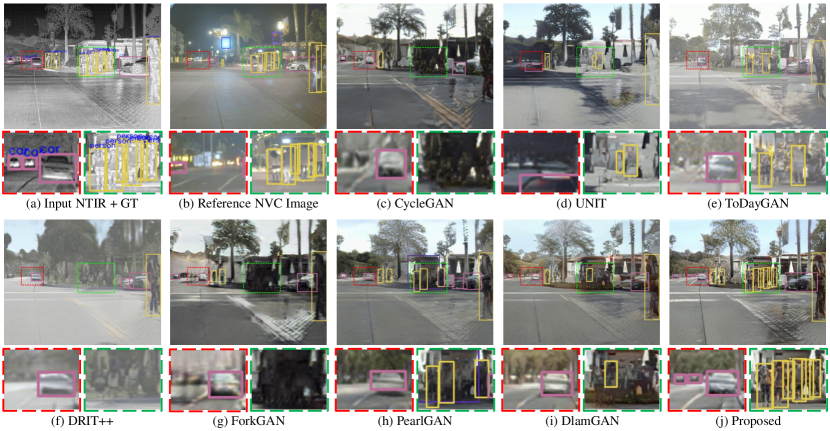
Although encouraging progress has been made in semantically consistent I2I translation, three important issues have not been fully considered. First, there has been little research on how to improve the texture realism of small sample objects (e.g., pedestrians and traffic signs) when there are no available semantic annotations for both domains. Second, how to reduce the high confidence noise in pseudo-labels when there is no available semantic annotation remains under-explored. Third, the problem of image gradient disappearance in local regions during translation is still under-addressed. As shown in Fig. 1, the popular NTIR2DC methods (e.g., PearlGAN [9] and DlamGAN [10])111As few available NTIR2DC methods exist, only the two methods mentioned are utilized here for comparison. fail to generate plausible pedestrians, as shown in the white dashed boxes. Moreover, the gradients of some trunk regions in their colorization results are vanishing, as shown in the red boxes. To address the above problems, we propose a Memory-guided cOllaboRative atteNtion GAN model (MornGAN).

We observe that the poor translation performance of small sample objects comes mainly from two aspects: the small number of total pixels and the difficulty of learning complex and variable texture features. Unlike deep neural networks, humans can efficiently identify a common relational system between two contexts and use these commonalities to make further inferences, which is called analogical reasoning [11]. Analogical reasoning is an important cognitive mechanism that involves retrieving structured knowledge from long-term memory and representing the binding of role-fillers in working memory [12]. Therefore, inspired by analogical reasoning mechanisms, we design a memory-guided collaborative attention approach to improve the translation performance, whose framework is shown in Fig. 2. In this framework, the semantic information of NTIR images is first obtained by an online semantic distillation process and then memorized online. Subsequently, cross-domain sample pairs containing similar objects are associated by a memory-guided sample selection strategy for collaborative learning. Finally, adaptive collaborative attention loss is introduced to encourage similarity in the feature distributions of objects in the same categories.
To reduce the high-confidence noise in the pseudo-labels of NTIR images, we devise an online semantic distillation module that consists of a label mining process and a semantic denoising process. The label mining process extracts the high-confidence part of the intersection of the segmentation predictions of two domains as the coarse labels. Then, the semantic denoising process refines the coarse labels using the distributional properties of the original NTIR images. To compensate for edge smoothing, we propose a conditional gradient repair loss to encourage the preservation of necessary edges. In addition, scale robustness loss is introduced to improve the robustness of the model for multi-scale objects.
The main contributions of this study are summarized as follows:
-
•
We propose a memory-guided sample selection strategy and an adaptive collaborative attention loss to improve the translation performance of small sample objects, which may provide novel research insights for few-shot domain adaptation and domain generalization.
-
•
An online semantic distillation module is devised to mine pseudo-labels for NTIR images, where the semantic denoising process can be generalized to other domains (e.g., visible spectrum) for pseudo-labels refinement.
-
•
A conditional gradient repair loss is introduced to reduce edge disappearance during translation, which is important for scene layout preservation.
-
•
Extensive experiments on the FLIR [13] and KAIST [14] datasets show that the proposed MornGAN222The source code will be available at https://github.com/FuyaLuo/MornGAN/. significantly outperforms other I2I translation methods in terms of semantic preservation and edge consistency, which remarkably improves the object detection accuracy.

The rest of this paper is organized as follows. Section 2 summarizes related work about TIR image colorization and I2I translation. Section 3 introduces the architecture of the proposed MornGAN. Section 4 presents the experiments on the FLIR and KAIST datasets. Section 5 draws the conclusions.
2 Related Work
In this section, we briefly review previous work on TIR image colorization, unpaired I2I translation, and memory networks.
2.1 TIR Image Colorization
TIR image colorization aims to map a single-channel grayscale TIR image to a three-channel RGB image based on the image content. With the recent successes of deep neural networks, a large number of methods have been proposed to handle TIR image colorization. In general, these methods can be classified as supervised or unsupervised methods. Supervised methods usually rely on matched cross-domain image pairs to maximize the similarity of the network output to the labels. For example, Berg et al. [15] leveraged separate luminance and chrominance loss to optimize the mapping of TIR images to colored visible images. In order to increase the naturalness of the results, researchers have made more attempts [16, 17, 18] to colorize TIR images based on pixel-level content loss by introducing additional adversarial loss. However, the difficulty of collecting pixel-level aligned paired samples limits the practicality of the supervised methods for TIR colorization tasks. In contrast, as they do not require paired samples, unsupervised methods usually utilize GAN models to make the generated images indistinguishable from real RGB images. For example, Nyberg et al. [19] exploited the CycleGAN [3] model to realize unpaired infrared-visible image translation. PearlGAN [9] was proposed to reduce semantic encoding entanglement and geometric distortion in the NTIR2DC task. DlamGAN [10] was designed with a dynamic label mining module to predict the semantic masks of NTIR images to encourage semantically consistent colorization. Despite the impressive progress, few efforts have been made to improve the colorization performance of small sample objects.
2.2 Unpaired I2I Translation
The purpose of unpaired I2I translation is to learn the mapping functions between different image domains using unpaired samples. Driven by the cycle consistency loss in CycleGAN [3], the unpaired I2I translation task has gained considerable attention in the computer vision community [4, 20, 21]. For example, MUNIT [22] and DRIT++ [23] were proposed to improve the diversity of synthesized images by learning a disentangled style representation and content representation. Anoosheh et al. [24] utilized multiple discriminators to improve the generation performance of night-to-day image translation. To reduce content distortion during translation, many researchers [5, 6, 8] have introduced semantic consistency loss using the available semantic annotations. When no semantic annotation is available for both domains, DlamGAN [10] first predicts the pseudo-labels of one domain using domain adaptation, and then introduces a dynamic label mining module to obtain the pseudo-labels of the other domain. Although semantic consistency loss can significantly reduce the semantic distortion during translation, the edges within or between classes of the background category are usually smoothed or disappear to enhance the realism of the image patches. However, this image texture vanishing problem is usually underappreciated. Moreover, how to reduce the high confidence noise in pseudo-labels using domain knowledge is still under-explored.
2.3 Neural Networks with External Memory
A memory network [25, 26] is a learnable neural network module that allows writing information to external memory and reading relevant content from memory slots. Due to their storage of long-term information and explicit memory manipulation, memory networks have been widely adopted in solving various computer vision problems such as few-shot learning [27, 28], semi-supervised learning [29], domain adaptation [30], and domain generalization [31]. For example, Xie et al. [27] proposed a recurrent memory network to directly learn to recursively read information from the support set features at all resolutions and capture features across resolutions to achieve more accurate few-shot semantic segmentation. Alonso et al. [29] used a memory bank to store and update the category-level features of labeled data, and constrain the category-level features of unlabeled data to be consistent with the memorized feature to achieve semi-supervised semantic segmentation. Furthermore, to improve the transfer performance of object features, VS et al. [30] exploited memory-guided attention maps to route target domain features into the corresponding category discriminators to ensure the domain alignment of category features. Jeong et al. [32] proposed a class-aware memory network to explicitly record category-level style differences for instance-level image translation using bounding-box annotation. Unlike existing methods, the proposed method does not require manual annotation of training data, and the introduction of memory units does not increase the computational cost of the inference stage.
3 Proposed Method

In this section, we first present the overview of MornGAN. Subsequently, we briefly explain our baseline model. Then, the details of online semantic distillation module are described. Next, we explicate the memory-guided collaborative attention mechanism, including the memory-guided sample selection strategy and adaptive collaborative attention (ACA) loss. Afterward, the conditional gradient repair (CGR) loss constraining edge consistency during translation is explained. Then, the scale robustness (SR) loss responsible for boosting the robustness of the model to object scale changes is specified. Finally, we illustrate the total loss of MornGAN.
In the rest of the paper, domain A and domain B denote the DC image set and NTIR image set, respectively. Taking the translation from domain A to domain B as an example, we denote the input image pair of domain A and B as , the generator contains an encoder of domain A and a decoder of domain B, and the discriminator aims to distinguish the real image from the translated image . Similarly, the inverse mapping includes generator and discriminator .
3.1 Model’s Overview and Problem Formulation
The overall framework is shown in Fig. 3. We first improve our previously developed ToDayGAN-TIR [9] model to accommodate subsequent semantic consistency requirements, which is called ToDayGAN-NTIR. Then, the ToDayGAN-NTIR model, containing a pair of generators and discriminators, is used as a baseline model with a total objective function consisting of adversarial loss , cycle-consistency loss , total variance loss , and structured gradient alignment (SGA) loss . Subsequently, we introduce two segmentation networks, and , to predict the segmentation masks of the images in both domains. The segmented pseudo-labels of the two domains, and , are obtained by the existing semantic segmentation model [33, 34] of DC images and the proposed online semantic distillation module, respectively. The pseudo-labels of NTIR images are subsequently stored in the memory unit. When the stored quantity meets the condition, the memory-guided sample selection strategy is triggered, and then similar NTIR images are recalled for the input DC images for collaborative learning. Finally, ACA loss constrains the inter-domain similarity of features of small sample classes. In addition, segmentation losses of synthesized images, denoted as and , are used to encourage semantically invariant image translation. To reduce edge degradation during translation, CGR loss is introduced. The SR loss aims to improve the insensitivity of the model to the object scale.
3.2 Baseline Model
3.2.1 Revisiting ToDayGAN-TIR Model
The ToDayGAN [24] model introduces three discriminators to improve the translation performance of visible images from nighttime to daytime. ToDayGAN-TIR [9] adapts ToDayGAN to improve the performance of NTIR image colorization. To avoid dot artifacts, ToDayGAN-TIR replaces the last two instance normalization layers of the decoder with group normalization [35] layers and combines the total variance [36] loss to reduce the noise of the translation results. To improve the representation ability of cycle-consistency loss for NTIR images, it introduces SSIM [37] loss based on the original L1-norm loss. In addition, it introduces the spectral normalization [38] layer into the discriminator to make the model training more stable. Similar to ToDayGAN, it chooses relativistic loss [39], adapted to least-squares GAN loss, as adversarial loss .
3.2.2 Generating High-quality Fake NTIR Images
To predict the semantic mask of NTIR images without available annotation, which is a necessary component for semantic consistency loss, we need high-quality fake NTIR images and corresponding DC image pseudo-labels to train the segmentation network for NTIR domain. Therefore, we first introduce SGA [9] loss to reduce the edge distortion during translation based on the ToDayGAN-TIR model. SGA loss encourages the ratio of the gradient of the synthesized image at the edge of the original image to the maximum gradient to be greater than a given threshold. In addition, to further obtain high-quality fake NTIR images, we introduce two regularization terms in the SGA loss of domain A, the monochromatic regularization term and the temperature regularization term. As the output fake NTIR image is three-channel data, the monochromaticity regularization term aims to encourage the values of the three channels to be the same. For the unnatural situation where the mean value of the pedestrian area in the fake NTIR image is extremely small, the temperature regularization term is responsible for encouraging the minimum value of the pedestrian area to be no less than the mean value of the road area. This regularization term is inspired by the observation that the body temperature of pedestrians is usually higher than the mean temperature of the road area during nighttime conditions.
Concretely, similar to [40], we first define the channel maximum operation as a mapping . Then, given the input , the output of the channel maximum operation at position can be expressed as
| (1) |
Next, the monochromatic regularization term can be denoted as
| (2) |
For the temperature regularization term, given the mean value of the road region of the fake NTIR image, denoted as , and the minimum value of the pedestrian region of the fake NTIR image, denoted as , the temperature regularization term can be represented as
| (3) |
where the denominator is intended to normalize the output in the range , and is a small value to avoid dividing by zero. Ultimately, the improved SGA loss can be expressed as
| (4) |
Combining the above two adjustments, we obtain the variant model ToDayGAN-NTIR, which serves as the baseline for MornGAN.
3.3 Pseudo-label Inference and Segmentation Loss
The above ToDayGAN-NTIR model still does not solve the problem of content distortion in the translation process. Therefore, similar to [5, 6], we introduce auxiliary segmentation networks (i.e, and ) and segmentation masks to encourage semantically consistent I2I translation. Due to the lack of manual annotation of both domains, similar to DlamGAN [10], we first obtain the pseudo-labels of domain A using the existing DC image segmentation model, and then design a label mining module to predict the pseudo-labels of NTIR images online.
Unlike DlamGAN, our proposed approach uses an online semantic distillation module that not only exploits different thresholds to balance the distribution bias among categories, but also utilizes the variation in temperature distribution among categories to reduce high-confidence noise.
3.3.1 Semantic Denoising
To obtain segmentation pseudo-labels for both domains, we first introduce a novel semantic denoising process that utilizes the class-specific low-rank properties of the original image to remove noisy labels that deviate from the distribution. For the specific category in the dataset, given the coarse pseudo-labels , the input image , and the set of confusion categories of , we can obtain a more trustworthy binary mask through the semantic denoising process. Specifically, for a given category , we first compute its binary mask and average pixel feature . Subsequently, we define the matrix of feature distances from pixels belonging to category to category as , and the value of at position can be formulated as
| (5) |
where denotes element-wise multiplication with channel-wise broadcasting, and the first term of the multiplication aims to ignore the feature distances of the locations that do not belong to category , while the second term is used to calculate the Euclidean distance between features. Ultimately, the value of at position can be given by
| (6) |
where is the indicator function (i.e., output 1 when the condition is met, and otherwise 0), and the equation in the indicator function determines whether the label at that location is noise by comparing the magnitude of the intra-class distance with that of the inter-class distance. In sum, the above semantic denoising process can be expressed using the mapping as
| (7) |
If there are multiple categories to be denoised, each category is updated with its own average feature after denoising, which enables a more reasonable estimation of the inter-class distance afterward. Two examples of SDP are shown in Fig. 4, and the fifth column shows the result of SDP on the fourth column.

3.3.2 Pseudo-label Inference of Visible Domain
As there is no segmentation label for DC images and the domain-adapted semantic segmentation methods still suffer from high-confidence noise, we directly utilize the existing segmentation models trained on different datasets to jointly predict the pseudo-labels of DC images. Concretely, we choose Detectron2 [33], a panoptic segmentation model trained on the MS COCO dataset [41], and HMSANet [34], a semantic segmentation model trained on the Cityscape dataset [42]. Due to the difference in training data, the Detectron2 model is good at object contour segmentation but is weaker than the HMSANet model for segmentation of traffic scene categories, as shown in the first row in Fig. 4. Therefore, we take the intersection of the predictions of HMSANet and Detectron2 as the pseudo-labels of the pedestrian, car, and building categories, and the predictions of HMSANet for the other categories. The pseudo-labels obtained by fusion are noted as .
However, we observe that the segmentation results after upsampling usually show shifting of edges and inflation of semantic regions due to the pooling and strided convolution operations in deep neural networks. In addition, there are significant low-rank properties (e.g., color homogeneity) within some background classes (i.e., tree, sky, and pole) in the visible domain with large inter-class differences. Accordingly, we exploit the distributional properties of these categories to reduce the noise in the pseudo-labels. Specifically, assuming that the categories of tree, pole, and sky are denoted as , and , respectively, the pseudo-labels of these three categories are refined sequentially using the semantic denoising process mentioned above; that is, , and . Because the semantic edges of trees and poles usually expand into the sky region in the predicted segmentation masks, the set of confusion categories , , and are , , and , respectively. After denoising, we can obtain the pseudo-labels of the DC image. An example image after denoising is shown in the fifth column of the first row in Fig. 4, and the final pseudo-labels can significantly reduce the predicted noise.
3.3.3 Online Semantic Distillation Module
With the obtained pseudo-labels of DC images, we can train the segmentation network with input , and with input . After that, we devise an online semantic distillation module to jointly predict the pseudo-labels of NTIR images by using and . The online semantic distillation module consists of a label mining process and a semantic denoising process, where the former mines the high-confidence part of the network prediction intersection as the coarse pseudo-labels, and the latter denoises the pseudo-labels based on the category distribution properties. Concretely, we first define the probability tensor of outputs and as and , respectively, whose values at the channel and at position denote the probability that the position belongs to category , denoted as and . Moreover, denotes the number of categories. Considering the difference in the number of categories and the fact that GAN models usually translate object regions in IR images into background regions to enhance the realism of synthesized images [9], label mining using the same threshold for all categories is suboptimal. Therefore, we design two thresholds, and , to extract the pseudo-labels of the foreground category and background category , respectively. Then, the category of pseudo-labels at location obtained by the label mining process, denoted as , can be represented as
| (8) |
And is a category-dependent piecewise function:
| (9) |
Due to the presence of high confidence noise in the label mining results, we exploit the semantic denoising process to suppress the noisy labels similar to how we handle pseudo-labels of DC images. Considering that the body temperature of pedestrians is usually significantly higher than some of the background categories (e.g., trees) in the nighttime environment, we add denoising for the pedestrian region to the three background categories (i.e., trees, poles, and sky) mentioned in the previous subsection. Specifically, we first abbreviate the pedestrian category as . Then, we use Eq. (7) to denoise the four categories of sky, pole, pedestrian and tree in turn, i.e., , , , . Considering the spatial distribution of the categories, the set of confusion categories , , , and is set to , , , and , respectively. After denoising, we can obtain the pseudo-labels of the NTIR image, denoted as . An example diagram of the online semantic distillation module is shown in the second row in Fig. 4.
3.3.4 Segmentation Loss
Pseudo-labels of both domains are used not only for supervising the training of the segmentation network, but also for encouraging semantically invariant image translation. Both stages require segmentation loss as the optimization objective. Due to the uneven distribution among categories, we utilize a modified pixel-level cross-entropy loss [43] as the segmentation loss for the three branches (i.e., , , and ), which assigns larger weights for smaller sample categories. Thanks to the sharp edges in the DC images and the relatively complete semantic edges in the pseudo-labels, we can improve the edge segmentation performance of model by introducing boundary loss. Referring to [44], the absolute value of the difference between the original image and the result after average pooling is taken as the spatial gradient. Then, we can calculate the difference in the spatial gradient between the predicted semantic probability tensor and the label, whose absolute value is taken as the boundary loss. Thus, the loss consists of a modified pixel-level cross-entropy loss [43] and a boundary loss [44], where the weight of the boundary loss is empirically set to 0.5. Ultimately, the complete segmentation loss can be expressed as
| (10) |
where , , , and are binary (i.e., either 0 or 1) loss weights used to switch learning stages.
3.4 Memory-guided Collaborative Attention
Although the online semantic distillation module and segmentation loss can help reduce the semantic distortion during translation, how to improve the translation performance of small sample categories remains to be explored. We observe that regions of small-sample categories in DC images have relatively complete semantic masks, which are usually fragmented for NTIR images. However, humans are usually good at combining memory and similarities between two situations to solve such small sample inference problems [11, 12], which is called the analogical reasoning mechanism. Inspired by this insight, we design a memory-guided collaborative attention mechanism to improve the colorization performance of small sample categories , which consists of a memory-guided sample selection strategy and an adaptive collaborative attention loss.
3.4.1 Memory-guided Sample Selection Strategy
The memory-guided sample selection strategy aims to select cross-domain sample pairs containing objects of the same categories for collaborative learning. Due to the lack of semantic labels of NTIR images, online memorization of semantic masks of NTIR images is necessary. Therefore, as shown in Fig. 3, after the weights of the segmentation network are fixed, we leverage the online semantic distillation module to infer the pseudo-label of the NTIR image, which is subsequently stored in the memory unit. After the semantic masks of all NTIR images are stored, the sample selection strategy works to select the appropriate NTIR images for a given DC image based on the distribution similarity.
As the goal is to improve the colorization performance of small sample categories, the focus is on the similarity of the distribution of cross-domain sample pairs in small sample categories. Concretely, given the semantic mask of a DC image, we first calculate the percentage of regions corresponding to each small sample category relative to the full image, and then subtract the mean value to obtain the vector as the semantic distribution feature. Similarly, we can obtain the semantic distribution feature of any NTIR image. Further, the similarity of the distribution between and , denoted as , can be expressed using the folldue cosine similarity:
| (11) |
where represents the L2 norm.
Although we can use similarity to find the NTIR image with the most similar (i.e., top-1 selection) distribution for the given DC image, the incompleteness of may lead to frequent selection of a particular NTIR image, which can cause overfitting of the model. To avoid this problem, the top-1 selection strategy is relaxed to random sampling from the top-k candidates, which means that one of the most similar NTIR images is randomly selected for collaborative learning with the given DC image. Unlike the popular learning method of random sample pairs in GAN models [2], the proposed collaborative learning approach can pave the way for subsequent category-aware cross-domain constraints.
3.4.2 Adaptive Collaborative Attention (ACA) Loss
With the selection of cross-domain sample pairs containing small sample categories, an ACA loss is designed to further encourage the similarity of feature distributions within classes. Due to the complexity of the constituent parts of object categories, characterizing the texture of objects with a single mean feature is sub-optimal. Accordingly, we first use Kmeans [45, 46] to extract the features of the components of the small sample categories of the real DC image. Then, the inner product between each component feature and the original feature is used to characterize the response map or co-attentive map of that component feature. Ultimately, the distance between the corresponding response maps of the fake and DC images is used to measure the similarity of the feature distributions. Specifically, we first denote the features of the real DC image and the fake DC image after the encoder as and , respectively, and their corresponding segmentation pseudo-labels as and , respectively. Given any category in the small sample category set , we can obtain the binary masks and of this category in two domains. Then, let the sum of non-zero elements in be , the feature matrix corresponding to the category in the real DC image can be denoted as
| (12) |
where denotes the operation of first transforming the input into a matrix of rows columns and then extracting the columns in which the sum of absolute values is non-zero. Subsequently, we utilize Kmeans to obtain the clustering feature matrix , where each row denotes the features of the cluster centroids, and denotes the number of clusters. Afterward, we can obtain the response map of all centroid features, which can be expressed using the cosine similarity between features as follows:
| (13) |
Then, we reshape into and . Further, the mean value of the maximum response of each location for all centroid features can be formulated as
| (14) |
Correspondingly, the mean value of the maximum response of each cluster for the features at all locations can be expressed as
| (15) |
Similarly, we can compute and using and . Thus, the ACA loss for category can be presented as
| (16) |
where and are the thresholds for controlling the local (i.e., individual centroid features) and global (i.e., distribution of centroid features) similarity between the features of the synthesized image and the centroid features, respectively. At last, the ACA loss for all small sample categories can be shown as
| (17) |
where denotes the total number of small sample categories.
3.5 Conditional Gradient Repair (CGR) Loss
Although the colorization performance of small sample classes can be improved by memory-guided collaborative attention mechanisms, the problem of image gradient disappearance during translation remains under-addressed. To better deceive the patch discriminator, the generator usually smooths the intra-class edges (e.g., lane lines and window frames) or inter-class edges of the background class (e.g., tree and sky) as texture regions, which severely deviates from the scene layout of the original image. Therefore, a CGR loss is designed to selectively preserve the gradient structure of the original image, which encourages the gradient value of the translated image to be not smaller than the gradient at the corresponding location of the original image. Considering the existence of noisy regions with small gradient values in the NTIR image, the CGR loss focuses only on the structural preservation of regions with relatively large gradients in background categories.
Due to the differences in the gradient distribution between images, we divide the gradients into two parts according to a sample-specific threshold (i.e., mean gradient value of the given image) rather than a fixed threshold. Specifically, the gradient maps of the NTIR image and its corresponding fake DC image are defined as and , respectively. Given the binary mask of the background region of the NTIR image, the gradient map of the background region can be denoted as
| (18) |
Similarly, we obtain the gradient map of the background region corresponding to the translated image, denoted as . Then, we calculate the average gradient of the background region, denoted as . After that, we obtain the binary mask with a gradient greater than . Finally, the CGR loss can be formulated as
| (19) |
where denotes the rectified linear unit. With CGR loss, the structural consistency between the colorization result and the original image is further enhanced.
3.6 Scale Robustness (SR) Loss
Inspired by self-supervised learning [47, 48], a SR loss is designed to improve the robustness of the model to variations in object scale, which encourages that the outputs corresponding to inputs of different scales can be resized to the same result. Concretely, taking domain A as an example, the inputs with scaled by factor and factor are denoted as and , respectively. Then, , , and are denoted as , and , respectively. As the temperature differences between background categories in NTIR images are small, with reference to [9], we use the smooth L1 loss [3] and SSIM [37] loss to jointly capture the differences between images. Thus, given the inputs and , the corresponding SR loss can be expressed as
| (20) |
where denotes the weight of smooth L1 loss, and denotes down-sampling of folds. Similarly, given the inputs and , the corresponding SR loss, denoted as , can be formulated as
| (21) |
Further, the SR loss of domain A can be expressed as
| (22) |
where denotes a random variable within varying with epoch. Similarly, we can obtain the SR loss for domain B. Finally, the total SR loss is the sum of and . With the introduction of SR loss, the problem of intra-class semantic inconsistency of large scale objects in translation results is further reduced.
3.7 Objective Function
4 Experiments
In this section, we first introduce the datasets and evaluation metrics associated with the NTIR2DC task. Then, we describe the experimental settings and implementation details. Experimental results on the FLIR and KAIST datasets are then presented. Afterward, we perform an ablation analysis of the proposed modules, losses, and strategies. The discussion of the experiments is provided at the end.
4.1 Datasets and Evaluation Metrics
4.1.1 Datasets
The FLIR and KAIST datasets are two commonly used benchmarks for the NTIR2DC task. The FLIR Thermal Starter Dataset [13] provides TIR images with bounding box annotations for training and validation of the object detection model, while the reference RGB images are unannotated. Through the same data split as in [9], we finally obtain 5447 DC images and 2899 NTIR images for training, while an additional 490 NTIR images are used for testing.
The KAIST Multispectral Pedestrian Detection Benchmark [14] provides coarse-aligned RGB and TIR image pairs, which contain both daytime and nighttime conditions. Folldue [9], the training set contains 1674 enhanced DC images and 1359 NTIR images, and an additional 500 NTIR images are used as the test set to evaluate the semantic and edge consistency. For the pedestrian detection experiments, the sample size of the test set is 611.
In order to remove the black areas on both sides in some images, according to [9], we first resize the training images to a resolution of , and then the resolution images obtained by center cropping are used as training data.
4.1.2 Evaluation Metrics
To evaluate the performance for image content preservation at each level, we conduct experiments on three vision tasks: semantic segmentation, object detection, and edge preservation.
Intersection-over-Union (IoU) [49] is a widely used metric in semantic segmentation tasks. The mean value of IoU for all classes, denoted as mIoU, is adopted to evaluate the semantic consistency of NTIR image colorization methods.
Average precision (AP) [50] denotes the average detection precision of the object detection model under different recalls. The mean value of AP for all categories, defined as mAP, is selected as an overall evaluation metric.
APCE [9] is the average precision of Canny edges under multi-threshold conditions, and is employed to evaluate the edge preservation performance of the NTIR2DC model.
4.2 Experimental Settings and Implementation Details
We compare MornGAN with other NTIR2DC methods such as PearlGAN [9] and DlamGAN [10], as well as some low-light enhancement methods (e.g., ToDayGAN [24] and ForkGAN [20]) and prevalent I2I translation methods (e.g., CycleGAN [3], UNIT [4] and DRIT++ [23]). We follow the instructions of these methods in order to establish a fair setting for comparison.
MornGAN is implemented using PyTorch. We train the models using the Adam [51] optimizer with on NVIDIA RTX 3090 GPUs. The batch size is set to 1 for all experiments. The learning rate of the whole training process is maintained at 0.0002. The total number of training epochs for the FLIR and KAIST datasets are 80 and 160, respectively. In Eq. (9), the pseudo-label thresholds and are empirically set to 0.95 and 0.99, respectively, and includes buildings and all object categories, while the remaining categories all belong to . In subsection 3.4, includes six categories: traffic light, traffic sign, person, truck, bus, and motorcycle. The number of clusters (i.e., ) for Kmeans clustering in ACA loss is set to four. In Eq. (16), the similarity thresholds and are both set to 0.9 to enhance the feature similarity within the classes. In subsection 3.6, the scale factors and are set to 0.5 and 1.5, respectively, to reduce the sensitivity of the model to object scale. For data augmentation, we flip the images horizontally with a probability of 0.5, and randomly crop them to . The number of parameters of our model is about 46.7 MB, and the inference speed on an NVIDIA RTX 3090 GPU is about 0.01 seconds for an input image with a resolution of pixels.
To achieve semantic consistency in translation, similar to DlamGAN [10], we divide the training process corresponding to segmentation loss into three phases333See https://github.com/FuyaLuo/MornGAN/ for specific implementation details.: learning , learning , and constraining semantic consistency after fixing and .
Due to the lack of pixel-level annotations in the FLIR and KAIST datasets, we evaluate the semantic segmentation performance of translated images using a scene parsing model [34] trained on Cityscape [42], which considers both the feature plausibility and semantic consistency of colorization. Similarly, to measure the naturalness of object features, we utilize YOLOv4 [52], which is trained on the MS COCO [41] dataset as the evaluation model for object detection.

| Road | Building | Sky | Car | Traffic Sign | Pedestrian | Motorcycle | Truck | Bus | mIoU | |
|---|---|---|---|---|---|---|---|---|---|---|
| Reference NVC image | 95.2 | 53.7 | 1.0 | 56.6 | 5.2 | 40.3 | 0.0 | 2.5 | 70.1 | 36.1 |
| CycleGAN [3] | 97.2 | 19.6 | 89.4 | 79.3 | 0.0 | 67.1 | 0.0 | 0.3 | 0.8 | 39.3 |
| UNIT [4] | 96.3 | 48.3 | 92.5 | 63.7 | 0.0 | 59.5 | 12.4 | 0.6 | 49.4 | 47.0 |
| ToDayGAN [24] | 97.0 | 42.3 | 83.2 | 76.5 | 0.0 | 56.3 | 2.5 | 0.0 | 6.5 | 40.5 |
| DRIT++ [23] | 98.2 | 16.1 | 75.3 | 79.4 | 0.0 | 38.3 | 0.0 | 0.0 | 3.2 | 34.5 |
| ForkGAN [20] | 96.2 | 48.9 | 90.2 | 82.1 | 0.0 | 73.2 | 7.9 | 0.0 | 17.8 | 46.3 |
| PearlGAN [9] | 98.6 | 71.0 | 95.1 | 89.1 | 0.0 | 84.3 | 12.2 | 1.5 | 0.0 | 50.2 |
| DlamGAN [10] | 97.4 | 67.2 | 94.0 | 89.1 | 0.1 | 74.0 | 36.2 | 2.1 | 0.3 | 51.2 |
| Proposed | 98.7 | 84.0 | 96.8 | 95.6 | 0.7 | 94.5 | 40.4 | 1.2 | 22.8 | 59.4 |
4.3 Experiments on the FLIR Dataset
4.3.1 Semantic Segmentation
The translation results and corresponding semantic outputs of various methods are shown in Fig. 5. Column (a) represents the reference nighttime visible color (NVC) image and its semantic segmentation. The segmentation model fails to discriminate the pedestrians on the side of the car due to the bright beam of car headlights and low surrounding illumination. As shown in the white dashed boxes in the second row, all the compared I2I translation methods fail to generate plausible pedestrians. In contrast, the proposed model can maintain the complete pedestrian region and pose to facilitate the segmentation model’s discrimination, whether it covers a crowd (e.g., left side of the road) or an isolated pedestrian (e.g., right side of the road). Furthermore, the proposed approach outperforms other compared approaches for the structural preservation of the unlabeled sidewalk category (i.e., the pink region in the semantic mask).
Table I reports the quantitative comparison of the semantic consistency of various translation models. The proposed MornGAN outperforms other methods in terms of semantic retention in four large sample categories (i.e., road, building, sky, and car) and three small sample categories (i.e., traffic sign, pedestrian, and motorcycle). As there are few available samples and diverse colors, all methods have poor translation performance for the traffic sign, truck, bus, and motorcycle categories. Benefiting from a memory-guided collaborative attention strategy, the proposed method slightly outperforms other methods in semantic preservation for traffic signs and motorcycles. However, due to the lack of spatial continuity constraints on large object representation, the proposed method produces limited improvement in translation performance for truck and bus. Overall, the proposed method outperforms the other methods by a significant margin (i.e., at least 8.2%) in terms of mIoU for scene layout maintenance.
4.3.2 Object Detection
Better translation should facilitate better object detection. Fig. 6 presents the qualitative comparison of the colorization and object detection by YOLOv4 [52] on the translated images of various I2I translation methods. As shown in the red dashed boxes, almost all methods fail to reasonably translate the distant car except ours, which demonstrates the superiority of the proposed method for small object preservation. For the translation of the occluded objects, as shown in the green dashed boxes, all the I2I translation methods fail to make YOLOv4 recognize the complete six pedestrians except ours. Although YOLOv4 can identify pedestrians in well-lit areas of the NVC image, it cannot identify pedestrians in low-light areas (i.e., the area between the red dashed box and the green dashed box in the original image), which can be complemented by the proposed method.
As the bounding-box annotation of the FLIR dataset covers only three categories (i.e., pedestrian, bicycle, and car), quantitative comparison of the various colorization results for object detection is shown in Table II. The proposed method outperforms the other methods by a clear margin in object preservation for all categories. For example, MornGAN outperforms the second-ranked PearlGAN by a significant margin of 13.1%, which indicates the superiority of our method in object retention.
| Pedestrian | Bicycle | Car | mAP | |
|---|---|---|---|---|
| Reference NVC image | 9.8 | 2.6 | 11.5 | 8.0 |
| CycleGAN [3] | 17.8 | 1.9 | 37.2 | 19.0 |
| UNIT [4] | 16.3 | 9.5 | 18.3 | 14.7 |
| ToDayGAN [24] | 19.0 | 1.5 | 53.3 | 24.6 |
| DRIT++ [23] | 16.5 | 2.2 | 46.0 | 21.6 |
| ForkGAN [20] | 25.9 | 2.3 | 32.5 | 20.2 |
| PearlGAN [9] | 54.0 | 23.0 | 75.5 | 50.8 |
| DlamGAN [10] | 48.0 | 17.8 | 70.2 | 45.4 |
| Proposed | 79.5 | 29.5 | 82.9 | 63.9 |
4.3.3 Edge Preservation
Fig. 7 visually compares the edge consistency of various translation methods. As shown in the blue dashed boxes, the edges of the buildings in the results of CycleGAN, ToDayGAN and DRIT++ are outwardly expanded, while the edges of the trees in the other four compared methods are inwardly shrunken. On the contrary, our model provides a complete match to the edges of the original image. In addition, as shown in the orange dashed boxes, ForkGAN, PearlGAN, and DlamGAN fail to maintain the continuous structure of the pole, and the edges of the pole are inwardly contracted in the other four methods. Compared with the other methods, MornGAN can more faithfully adhere to the edge structure of the original image.
As the Canny edges in the Fig. 7 are only the results of a fixed threshold, we exploit the APCE metric, which covers multiple thresholds to comprehensively evaluate the edge consistency performance, as shown in Fig. 8(a). We can find that the proposed method significantly outperforms other methods in edge consistency at all thresholds and is far superior to the second ranked DlamGAN by 18%.

4.4 Experiments on the KAIST Dataset
Different from FLIR [13], KAIST [14] is a more challenging dataset with low-contrast and blurred NTIR images.
| Road | Building | Sky | Car | Traffic Sign | Pedestrian | Motorcycle | Bus | mIoU | |
|---|---|---|---|---|---|---|---|---|---|
| Reference NVC image | 82.6 | 74.6 | 0.0 | 56.1 | 0.0 | 19.0 | 0.0 | 0.0 | 29.0 |
| CycleGAN [3] | 83.5 | 25.0 | 64.1 | 39.4 | 0.0 | 8.9 | 0.1 | 0.0 | 27.6 |
| UNIT [4] | 92.3 | 59.3 | 81.0 | 60.3 | 0.0 | 23.8 | 0.0 | 0.0 | 39.6 |
| ToDayGAN [24] | 92.5 | 57.6 | 82.8 | 54.1 | 3.6 | 23.3 | 0.1 | 0.0 | 39.3 |
| DRIT++ [23] | 89.1 | 58.9 | 63.1 | 47.6 | 0.0 | 5.6 | 0.0 | 0.0 | 33.0 |
| ForkGAN [20] | 89.6 | 30.3 | 44.6 | 48.5 | 0.5 | 27.9 | 0.0 | 0.0 | 30.2 |
| PearlGAN [9] | 93.4 | 43.1 | 83.8 | 70.3 | 0.9 | 57.6 | 0.0 | 6.1 | 44.4 |
| DlamGAN [10] | 92.6 | 49.0 | 71.9 | 66.4 | 2.1 | 49.5 | 2.0 | 8.2 | 42.7 |
| Proposed | 93.7 | 72.2 | 87.6 | 72.5 | 7.2 | 61.1 | 4.2 | 13.1 | 51.5 |

4.4.1 Semantic Segmentation
Fig. 9 visually compares the colorization results of various translation methods on the KAIST dataset and their segmentation outputs. The relatively reasonable segmentation results in column (a) demonstrate the applicability of the selected segmentation model proposed in [34]. However, as shown in the white dashed boxes, all the compared I2I translation methods are unable to generate realistic pedestrians for the segmentation model to discriminate. Instead, the proposed method not only maintains most of the semantics of the dashed box region but also provides partial clues for distant pedestrian detection.
Further, a quantitative comparison of the semantic preservation performance of various I2I translation methods is shown in Table III. Despite the poor image quality, which makes scene understanding extremely difficult, MornGAN achieves the best performance among all methods in terms of semantic preservation for each category. Similar to the results on the FLIR dataset, all I2I translation methods have poor semantic retention in small sample categories. With the help of the proposed learning approach, features of small sample categories can be better retained compared with other methods. Overall, the semantic consistency of MornGAN on the NTIR2DC task is far superior to that of other I2I translation methods, that is, at least 7.1% ahead.

4.4.2 Pedestrian Detection
For pedestrian preservation, a qualitative comparison of various translation methods on the KAIST dataset is shown in Fig. 10. As shown in the two dashed boxes, all the methods cannot maintain realistic and complete pedestrian features to make the detection model convincing. However, MornGAN can generate plausible features for near pedestrians while maintaining a relatively reasonable local feature distribution for distant pedestrians.
Further, the quantitative comparison for pedestrian preservation is shown in Table IV. Due to the large number of pedestrians and good lighting conditions in city scenes, the performance of pedestrian detection in the reference NVC images is slightly better than that of the proposed method. Nevertheless, MornGAN outperforms other methods both in terms of detection precision and recall, and has substantial advantages in terms of overall mAP metrics.

| Precision | Recall | mAP | |
|---|---|---|---|
| Reference NVC image | 36.8 | 50.1 | 44.2 |
| CycleGAN [3] | 4.7 | 2.8 | 1.1 |
| UNIT [4] | 26.7 | 14.5 | 11.0 |
| ToDayGAN [24] | 11.4 | 14.9 | 5.0 |
| DRIT++ [23] | 7.9 | 4.1 | 1.2 |
| ForkGAN [20] | 33.9 | 4.6 | 4.9 |
| PearlGAN [9] | 21.0 | 39.8 | 25.8 |
| DlamGAN [10] | 26.1 | 32.0 | 23.0 |
| Proposed | 34.3 | 52.7 | 42.6 |
4.4.3 Edge Preservation
Fig. 11 qualitatively compares the edge consistency of various translation methods on the KAIST dataset. Column (b) shows the enhanced NTIR image overlapped with Canny edges. As shown in the orange dashed boxes, the streetlights are vanishing in the results of ToDayGAN and DRIT++, while the edges of the streetlights are indented in the results of UNIT, ForkGAN, and PearlGAN. The neighboring structures of streetlights in CycleGAN and DlamGAN deviate severely from the input NTIR image. Similarly, as shown in the blue dashed boxes, the structures of the poles in the results of PearlGAN and DlamGAN are disconnected, while the streetlights and their neighboring edges of other methods differ significantly from the original image. Instead, our results match well with the original image on the edges.
Furthermore, the edge consistency comparison under the multi-threshold condition is shown in Fig. 8 (b). Considering all the thresholds, the proposed method still exhibits high performance in the edge consistency of the translation.


4.5 Ablation Study
Ablation analysis is performed on the FLIR dataset to discuss the validity of each component of MornGAN. The results of the ablation analysis are shown in Table V, and an example of a qualitative comparison is shown in Fig. 12. We can find from Fig. 12 that the baseline model has poor content preservation performance for the input and tends to generate more erroneous regions of the tree (e.g., the yellow box region in the second column). With the introduction of semantic consistency loss, the semantic retention performance of the small-sample object class is degraded by the presence of excessive noise in the pseudo-labels, despite the improvement of the overall semantic consistency. Moreover, the wrong semantic labels lead to degradation of edge consistency, as shown in the green box in the third column in Fig. 12.
In the next experiment, we perform SDP on the pseudo-labels, and the semantic preservation as well as edge consistency of the results are improved, as shown in the fourth column of Fig. 12. Then, due to the benefits of the MGCA strategy, the semantic preservation for the small sample category can be significantly improved, that is, a 3.4% gain, as shown in Table V.
With the introduction of CGR loss, the edge structure of the street light is clearer compared to the previous results, as shown in the green box in the sixth column of Fig. 12. The results in Table V further demonstrate the effectiveness of CGR loss for improving edge consistency.
Ultimately, as shown in the green box in the last column of Fig. 12, the SR loss can facilitate the structure of the pole matching that of the original image. Moreover, as shown in the red box and the black dashed box, the proposed method can generate more plausible pedestrians and reduce the content distortion. Compared with the baseline model, the proposed MornGAN can substantially improve the performance for image content and edge preservation without increasing model parameters.
| Baseline | SC | SDP | MGCA | CGR | SR | mIoU.A(%) | mIoU.S(%) | APCE |
|---|---|---|---|---|---|---|---|---|
| ✓ | 50.5 | 23.8 | 0.38 | |||||
| ✓ | ✓ | 51.8 | 20.5 | 0.37 | ||||
| ✓ | ✓ | ✓ | 54.0 | 23.6 | 0.39 | |||
| ✓ | ✓ | ✓ | ✓ | 56.8 | 27.0 | 0.43 | ||
| ✓ | ✓ | ✓ | ✓ | ✓ | 58.5 | 30.8 | 0.58 | |
| ✓ | ✓ | ✓ | ✓ | ✓ | ✓ | 59.4 | 31.9 | 0.58 |
4.6 Discussion
In this section, we analyze the generalization capability of the proposed method, the impact of the cluster number in the ACA loss on the results, and the limitations of MornGAN.
4.6.1 Generalization Experiments
In order to explore the generalization ability of various I2I translation methods to out-of-domain distributions, we apply each model trained on the KAIST dataset to the FLIR dataset abbreviated as KF and vice versa as FK. The results are shown in Table VI. For the performance of semantic preservation, we can find that the proposed method obtains the best mIoU among all methods for both KF and FK experiments. Similarly, for the comparison of edge consistency during translation, MornGAN outperforms other compared methods by a significant margin for APCE in both experimental paradigms. In summary, the results demonstrate the strong generalization capability of the proposed method for domain shift.
| mIoU(%) | APCE | |||||
|---|---|---|---|---|---|---|
| KF | FK | AVE. | KF | FK | AVE. | |
| CycleGAN [3] | 15.8 | 23.4 | 19.6 | 0.07 | 0.09 | 0.08 |
| UNIT [4] | 23.9 | 19.3 | 21.6 | 0.18 | 0.22 | 0.20 |
| ToDayGAN [24] | 27.9 | 18.5 | 23.2 | 0.09 | 0.10 | 0.10 |
| DRIT++ [23] | 12.5 | 23.0 | 17.8 | 0.06 | 0.14 | 0.10 |
| ForkGAN [20] | 39.0 | 15.1 | 27.1 | 0.23 | 0.10 | 0.17 |
| PearlGAN [9] | 37.8 | 28.5 | 33.2 | 0.21 | 0.24 | 0.23 |
| DlamGAN [10] | 32.4 | 20.2 | 26.3 | 0.18 | 0.30 | 0.24 |
| Proposed | 39.9 | 41.6 | 40.8 | 0.29 | 0.45 | 0.37 |
4.6.2 The Effect of Cluster Number on The Results
The effect of the cluster number in ACA loss on the colorization performance is shown in Table VII. When the number of clusters is small, the features of small sample objects are difficult to capture comprehensively, so the segmentation model fail to understand the presence of objects. However, when the number of clusters is too large, many irrelevant features in the objects may disturb the recognition of the segmentation model. Compared with semantic consistency, edge consistency during translation is less sensitive to the cluster number. Therefore, we set the cluster number to four in all experiments.
| Cluster Number | 2 | 3 | 4 | 5 | 6 |
|---|---|---|---|---|---|
| mIoU.A (%) | 57.1 | 58.6 | 59.4 | 55.5 | 56.7 |
| mIoU.S (%) | 28.0 | 30.2 | 31.9 | 26.1 | 26.2 |
| APCE | 0.56 | 0.58 | 0.58 | 0.57 | 0.59 |
4.6.3 Failure Cases
Fig. 13 shows four failure cases of MornGAN, where the input images in the first two columns are from the FLIR dataset, and the remaining images are from the KAIST dataset. As shown in the first and third columns, local areas of large scale pedestrians and cars are incorrectly translated as roads due to their similarity in temperature. Moreover, the model fails in generating plausible objects when the objects are close to the camera, as shown in the second and fourth columns. Therefore, more attempts should be made in the future to design reasonable modules to capture complete object representations, such as combining the integrity and continuity of Gestalt laws.

5 Conclusion
In this work, we developed a new learning framework called MornGAN to achieve colorization of NTIR images. Benefiting from the proposed memory-guided sample selection strategy and adaptive collaborative attention loss, the framework enabled the great improvement of the translation performance of small sample classes. The online semantic distillation module was designed to mine and refine the pseudo-labels of NTIR images. In addition, we devised a conditional gradient repair loss for avoiding image gradient disappearance during translation. Scale robustness loss was introduced to improve the robustness of the model to scale variation. Experiments on the NTIR2DC task demonstrated the superiority of the proposed approach in terms of semantic preservation and edge consistency, which remarkably improved the object detection performance on the translated images. Although the proposed semantic denoising process was only applied to a few categories with the low-rank property, its unsupervised and threshold-free advantages make it easy to extend to other tasks (e.g., saliency detection and image matting). In the future, it is a promising direction to further improve the reliability of scene parsing of NTIR images under weakly supervised conditions to ensure the semantic consistency of NTIR2DC tasks.
Acknowledgments
This work was supported by Key Area R&D Program of Guangdong Province (2018B030338001) and National Natural Science Foundation of China (61806041, 62076055).
References
- [1] G. W Stuart and P. K Hughes, “Towards an understanding of the effect of night vision display imagery on scene recognition,” The Ergonomics Open Journal, vol. 2, no. 1, 2009.
- [2] I. J. Goodfellow, J. Pouget-Abadie, M. Mirza, B. Xu, D. Warde-Farley, S. Ozair, A. C. Courville, and Y. Bengio, “Generative adversarial nets,” in Proc. NeurIPS, 2014.
- [3] J.-Y. Zhu, T. Park, P. Isola, and A. A. Efros, “Unpaired image-to-image translation using cycle-consistent adversarial networks,” in Proc. ICCV, 2017, pp. 2223–2232.
- [4] M.-Y. Liu, T. Breuel, and J. Kautz, “Unsupervised image-to-image translation networks,” in Proc. NeurIPS, 2017.
- [5] S.-W. Huang, C.-T. Lin, S.-P. Chen, Y.-Y. Wu, P.-H. Hsu, and S.-H. Lai, “Auggan: Cross domain adaptation with gan-based data augmentation,” in Proc. ECCV, 2018, pp. 718–731.
- [6] A. Cherian and A. Sullivan, “Sem-gan: semantically-consistent image-to-image translation,” in Proc. WACV. IEEE, 2019, pp. 1797–1806.
- [7] L. Musto and A. Zinelli, “Semantically adaptive image-to-image translation for domain adaptation of semantic segmentation,” arXiv preprint arXiv:2009.01166, 2020.
- [8] F. Pizzati, R. d. Charette, M. Zaccaria, and P. Cerri, “Domain bridge for unpaired image-to-image translation and unsupervised domain adaptation,” in Proc. WACV, 2020, pp. 2990–2998.
- [9] F. Luo, Y. Li, G. Zeng, P. Peng, G. Wang, and Y. Li, “Thermal infrared image colorization for nighttime driving scenes with top-down guided attention,” IEEE Trans. Intell. Transp. Syst., 2022.
- [10] F. Luo, Y. Cao, and Y. Li, “Nighttime thermal infrared image colorization with dynamic label mining,” in International Conference on Image and Graphics. Springer, 2021, pp. 388–399.
- [11] D. Gentner and L. Smith, “Analogical reasoning. encyclopedia of human behavior, 1, 130-136,” 2012.
- [12] K. J. Holyoak, “Analogy and relational reasoning,” The Oxford Handbook of Thinking and Reasoning, p. 234, 2013.
- [13] F.A.Group, “Flir thermal dataset for algorithm training,” https://www.flir.co.uk/oem/adas/adas-dataset-form/, May 2019.
- [14] S. Hwang, J. Park, N. Kim, Y. Choi, and I. So Kweon, “Multispectral pedestrian detection: Benchmark dataset and baseline,” in Proc. CVPR, 2015, pp. 1037–1045.
- [15] A. Berg, J. Ahlberg, and M. Felsberg, “Generating visible spectrum images from thermal infrared,” in Proc. CVPR Workshops, 2018, pp. 1143–1152.
- [16] N. Bhat, N. Saggu, S. Kumar et al., “Generating visible spectrum images from thermal infrared using conditional generative adversarial networks,” in ICCES, 2020, pp. 1390–1394.
- [17] X. Kuang, J. Zhu, X. Sui, Y. Liu, C. Liu, Q. Chen, and G. Gu, “Thermal infrared colorization via conditional generative adversarial network,” Infrared Physics & Technology, p. 103338, 2020.
- [18] T. Le-Tien, T. H. D. Quang, H. Y. Vy, T. Nguyen-Thanh, and H. Phan-Xuan, “Gan-based thermal infrared image colorization for enhancing object identification,” in 2021 International Symposium on Electrical and Electronics Engineering (ISEE). IEEE, 2021, pp. 90–94.
- [19] A. Nyberg, A. Eldesokey, D. Bergstrom, and D. Gustafsson, “Unpaired thermal to visible spectrum transfer using adversarial training,” in Proc. ECCV, 2018, pp. 0–0.
- [20] Z. Zheng, Y. Wu, X. Han, and J. Shi, “Forkgan: Seeing into the rainy night,” in Proc. ECCV. Springer, 2020, pp. 155–170.
- [21] R. Chen, W. Huang, B. Huang, F. Sun, and B. Fang, “Reusing discriminators for encoding: Towards unsupervised image-to-image translation,” in Proc. CVPR, 2020, pp. 8168–8177.
- [22] X. Huang, M.-Y. Liu, S. Belongie, and J. Kautz, “Multimodal unsupervised image-to-image translation,” in Proc. ECCV, 2018, pp. 172–189.
- [23] H.-Y. Lee, H.-Y. Tseng, Q. Mao, J.-B. Huang, Y.-D. Lu, M. Singh, and M.-H. Yang, “Drit++: Diverse image-to-image translation via disentangled representations,” International Journal of Computer Vision, vol. 128, no. 10, pp. 2402–2417, 2020.
- [24] A. Anoosheh, T. Sattler, R. Timofte, M. Pollefeys, and L. Van Gool, “Night-to-day image translation for retrieval-based localization,” in ICRA, 2019, pp. 5958–5964.
- [25] J. Weston, S. Chopra, and A. Bordes, “Memory networks,” in 3rd International Conference on Learning Representations, ICLR 2015, San Diego, CA, USA, May 7-9, 2015, Conference Track Proceedings, Y. Bengio and Y. LeCun, Eds., 2015. [Online]. Available: http://arxiv.org/abs/1410.3916
- [26] S. Sukhbaatar, J. Weston, R. Fergus et al., “End-to-end memory networks,” Proc. NeurIPS, vol. 28, 2015.
- [27] G.-S. Xie, H. Xiong, J. Liu, Y. Yao, and L. Shao, “Few-shot semantic segmentation with cyclic memory network,” in Proc. ICCV, 2021, pp. 7293–7302.
- [28] Z. Wu, X. Shi, G. Lin, and J. Cai, “Learning meta-class memory for few-shot semantic segmentation,” in Proc. ICCV, 2021, pp. 517–526.
- [29] I. Alonso, A. Sabater, D. Ferstl, L. Montesano, and A. C. Murillo, “Semi-supervised semantic segmentation with pixel-level contrastive learning from a class-wise memory bank,” in Proc. ICCV, 2021, pp. 8219–8228.
- [30] V. VS, V. Gupta, P. Oza, V. A. Sindagi, and V. M. Patel, “Mega-cda: Memory guided attention for category-aware unsupervised domain adaptive object detection,” in Proc. CVPR, 2021, pp. 4516–4526.
- [31] Y. Chen, Y. Wang, Y. Pan, T. Yao, X. Tian, and T. Mei, “A style and semantic memory mechanism for domain generalization,” in Proc. ICCV, 2021, pp. 9164–9173.
- [32] S. Jeong, Y. Kim, E. Lee, and K. Sohn, “Memory-guided unsupervised image-to-image translation,” in Proc. CVPR, 2021, pp. 6558–6567.
- [33] Y. Wu, A. Kirillov, F. Massa, W.-Y. Lo, and R. Girshick, “Detectron2,” https://github.com/facebookresearch/detectron2, 2019.
- [34] A. Tao, K. Sapra, and B. Catanzaro, “Hierarchical multi-scale attention for semantic segmentation,” arXiv preprint arXiv:2005.10821, 2020.
- [35] Y. Wu and K. He, “Group normalization,” in Proc. ECCV, 2018, pp. 3–19.
- [36] L. I. Rudin, S. Osher, and E. Fatemi, “Nonlinear total variation based noise removal algorithms,” Physica D: nonlinear phenomena, vol. 60, no. 1-4, pp. 259–268, 1992.
- [37] Z. Wang, A. C. Bovik, H. R. Sheikh, and E. P. Simoncelli, “Image quality assessment: from error visibility to structural similarity,” IEEE Trans. Image Process., vol. 13, no. 4, pp. 600–612, 2004.
- [38] T. Miyato, T. Kataoka, M. Koyama, and Y. Yoshida, “Spectral normalization for generative adversarial networks,” arXiv preprint arXiv:1802.05957, 2018.
- [39] A. Jolicoeur-Martineau, “The relativistic discriminator: a key element missing from standard gan,” arXiv preprint arXiv:1807.00734, 2018.
- [40] Z. Ma, D. Chang, J. Xie, Y. Ding, S. Wen, X. Li, Z. Si, and J. Guo, “Fine-grained vehicle classification with channel max pooling modified cnns,” IEEE Trans. Veh. Technol., vol. 68, no. 4, pp. 3224–3233, 2019.
- [41] T.-Y. Lin, M. Maire, S. Belongie, J. Hays, P. Perona, D. Ramanan, P. Dollár, and C. L. Zitnick, “Microsoft coco: Common objects in context,” in Proc. ECCV, 2014, pp. 740–755.
- [42] M. Cordts, M. Omran, S. Ramos, T. Rehfeld, M. Enzweiler, R. Benenson, U. Franke, S. Roth, and B. Schiele, “The cityscapes dataset for semantic urban scene understanding,” in Proc. CVPR, 2016, pp. 3213–3223.
- [43] Z. Zheng and Y. Yang, “Unsupervised scene adaptation with memory regularization in vivo,” in Proc. IJCAI, 2020.
- [44] M. Zhen, J. Wang, L. Zhou, S. Li, T. Shen, J. Shang, T. Fang, and L. Quan, “Joint semantic segmentation and boundary detection using iterative pyramid contexts,” in Proc. CVPR, 2020, pp. 13 666–13 675.
- [45] J. MacQueen, “Classification and analysis of multivariate observations,” in 5th Berkeley Symp. Math. Statist. Probability, 1967, pp. 281–297.
- [46] S. Lloyd, “Least squares quantization in pcm,” IEEE Trans. Inf. Theory, vol. 28, no. 2, pp. 129–137, 1982.
- [47] T. Chen, S. Kornblith, M. Norouzi, and G. Hinton, “A simple framework for contrastive learning of visual representations,” in International conference on machine learning. PMLR, 2020, pp. 1597–1607.
- [48] C. Zhao, G. G. Yen, Q. Sun, C. Zhang, and Y. Tang, “Masked gan for unsupervised depth and pose prediction with scale consistency,” IEEE Trans. Neural Netw. Learn. Syst., vol. 32, no. 12, pp. 5392–5403, 2020.
- [49] M. Everingham, S. A. Eslami, L. Van Gool, C. K. Williams, J. Winn, and A. Zisserman, “The pascal visual object classes challenge: A retrospective,” International journal of computer vision, vol. 111, no. 1, pp. 98–136, 2015.
- [50] M. Everingham, L. Van Gool, C. K. Williams, J. Winn, and A. Zisserman, “The pascal visual object classes (voc) challenge,” International journal of computer vision, vol. 88, no. 2, pp. 303–338, 2010.
- [51] D. P. Kingma and J. Ba, “Adam: A method for stochastic optimization,” in ICLR (Poster), 2015.
- [52] A. Bochkovskiy, C.-Y. Wang, and H.-Y. M. Liao, “Yolov4: Optimal speed and accuracy of object detection,” arXiv preprint arXiv:2004.10934, 2020.
| Fu-Ya Luo received the B.S. degree in biomedical engineering from University of Electronic Science and Technology of China (UESTC), in 2015. He is now pursuing his Ph.D. degree in UESTC. His research interests include scene understanding, brain-inspired computer vision, weakly supervised learning, and image-to-image translation. |
| Yi-Jun Cao received the M.S. degree from the College of Electric and Information Engineering, Guangxi University of Science and Technology. Currently, he is working toward the Ph.D. degree with the College of Electric and Information Engineering, University of Electronic Science and Technology of China (UESTC). His area of research are visual SLAM and navigation. |
| Kai-Fu Yang received the Ph.D. degree in biomedical engineering from the University of Electronic Science and Technology of China (UESTC), Chengdu, China, in 2016. He is currently an associate research professor with the MOE Key Lab for Neuroinformation, School of Life Science and Technology, UESTC, Chengdu, China. His research interests include cognitive computing and braininspired computer vision. |
| Yong-Jie Li (Senior Member, IEEE) received the Ph.D. degree in biomedical engineering from University of Electronic Science and Technology of China (UESTC), in 2004. He is currently a Professor with the Key Laboratory for NeuroInformation of Ministry of Education, School of Life Science and Technology, UESTC. His research focuses on building of biologically inspired computational models of visual perception and the applications in image processing and computer vision. |