∎
22email: {yugeng, lanliang}@comp.hkbu.edu.hk
Memory-Efficient Factorization Machines via Binarizing both Data and Model Coefficients
Abstract
Factorization Machines (FM), a general predictor that can efficiently model feature interactions in linear time, was primarily proposed for collaborative recommendation and have been broadly used for regression, classification and ranking tasks. Subspace Encoding Factorization Machine (SEFM) has been proposed recently to overcome the expressiveness limitation of Factorization Machines (FM) by applying explicit nonlinear feature mapping for both individual features and feature interactions through one-hot encoding to each input feature. Despite the effectiveness of SEFM, it increases the memory cost of FM by times, where is the number of bins when applying one-hot encoding on each input feature. To reduce the memory cost of SEFM, we propose a new method called Binarized FM which constraints the model parameters to be binary values (i.e., 1 or ). Then each parameter value can be efficiently stored in one bit. Our proposed method can significantly reduce the memory cost of SEFM model. In addition, we propose a new algorithm to effectively and efficiently learn proposed FM with binary constraints using Straight Through Estimator (STE) with Adaptive Gradient Descent (Adagrad). Finally, we evaluate the performance of our proposed method on eight different classification datasets. Our experimental results have demonstrated that our proposed method achieves comparable accuracy with SEFM but with much less memory cost.
Keywords:
Factorization Machines Binary Models1 Introduction
Factorization Machines (FM) (Rendle,, 2010) is a popular method that can efficiently model feature interactions in linear time with respect to the number of features. While FM has been successfully applied in different predictive tasks, it is also be noted that FM fails to capture highly nonlinear patterns in the data because it only uses polynomial feature expansion for nonlinear relationship modeling (He and Chua,, 2017; Liu et al.,, 2017; Lan and Geng,, 2019; Chen et al.,, 2019). To address the expressiveness limitation of the FM model, different methods have been proposed: (1) Embedding neural networks into FM models (He and Chua,, 2017; Xiao et al.,, 2017; Guo et al.,, 2017): they use neural-network based approach to model feature interactions in a highly nonlinear way; (2) Locally Linear FM (LLFM) (Liu et al.,, 2017) and its extension (Chen et al.,, 2019): they use a local encoding technique to capture nonlinear concept based on the idea that nonlinear manifold behaves linearly in its local neighbors; (3) Subspace Encoding FM (SEFM) (Lan and Geng,, 2019): it captures the nonlinear relationships of individual features and feature interactions to the class label by applying explicit nonlinear feature mapping to each input feature.
Although these FM extensions have shown improved accuracy on different predictive tasks, the space and computational complexity of these methods are much higher than the original FM. This high space and computational complexities will limit their applications in resource-constrained scenarios, such as model deployment on mobile phones or IoT devices. We seek to develop a novel memory and computational efficient FM model that can capture highly nonlinear patterns in the data. In this paper, we focus on reducing the memory cost of SEFM. The core idea of SEFM is to apply one-hot encoding for each input feature, which can effectively model the relationship of individual features and feature interactions to the class label in a highly-nonlinear way. SEFM can achieve the same computational complexity as FM for model inference. However, with respect to the space complexity of the model parameters, SEFM increases the memory cost of FM model by times where is the number of bins when applying one-hot encoding to each input feature.
Motivated by recent works that reduce the memory cost of classification models by binarizing the model parameters (Hubara et al.,, 2016; Rastegari et al.,, 2016; Alizadeh et al.,, 2018; Shen et al.,, 2017), we propose to reduce the memory cost of SEFM by binarizing their model parameters. By constraining the model parameters of SEFM to be binary values (i.e., 1 or ), only one bit is required to store each parameter value. Therefore, our proposed method can significantly reduce the memory cost of SEFM. Note that our proposed method is different from Discrete FM (Liu et al.,, 2018) (DFM) which only binarizes the model parameter for pairwise feature interactions on the original feature space. Our method based on mapped feature space will have a higher expressiveness capacity than DFM. In addition, DFM focuses on regression loss and their proposed training algorithm can not be directly applied for the hinge loss or logloss which are popular for classification problems. In this paper, we propose to train our binarized FM model by using Straight Through Estimator (STE) (Bengio et al.,, 2013) with adaptive gradient descent (AdaGrad) (Duchi et al.,, 2011) which can apply to any convex loss function.
The contributions of this paper can be summarized as: First, we propose a novel method that can reduce the memory cost of SEFM by binarizing the model parameters. Second, since directly learning the binary model parameters is an NP-hard problem, we propose to use STE with Adagrad to effectively and efficiently obtain the binary model parameters. We provide a detailed analysis of our method’s space and computational complexities for model inference and compare it with other competing methods. Finally, we evaluate the performance of our proposed method on eight datasets. Our experimental results have clearly shown that our proposed method can get much better accuracy than FM while having a similar memory cost. The results also show that our proposed method achieves comparable accuracy with SEFM but with much less memory cost.
2 Preliminaries
Factorization Machines. Given a training data set , where is a dimensional feature vector representing the -th training sample, is the class label of the -th training sample. denotes the -th feature value of the -th sample. The predicted value for a data sample based on FM with degree-2 is,
| (1) |
where models the relationship between the -th feature and the class label, and models the relationship between the pairwise feature interaction of feature and feature and the class label. In FM, the model coefficient for feature interaction is factorized as , where is an -dimensional vector. By using this factorization, the second term in (1) can be computed in time which is in linear with respect to the number of feature according to Lemma 3.1 in Rendle, (2010),
| (2) |
The model parameters of FMs are and . These model parameters can be efficiently learnt from data by using Stochastic Gradient Descent (SGD). The gradient of FM prediction based on one sample can be computed as
| (3) |
By using low rank factorization of , FM can model all pairwise feature interations in time which is much more efficient than SVM with polynomial-2 kernel Chang et al., (2010).


Subspace Encoding Factorization Machines. As shown in (1), the relationship of individual features and feature interactions to the class label in FM is just linear and therefore it fails to capture highly nonlinear pattern in the data. Recently, SEFM Lan and Geng, (2019) was proposed to address the expressiveness limitation of FM. The basic idea of SEFM is to apply one-hot encoding to each individual feature. This simple idea does an efficient non-parametric nonlinear feature mapping for both individual features and feature interactions and therefore can improve the model expressiveness capacity. For a given data sample , SEFM will transform it to a very sparse vector with length by using one-hot encoding where is the number of bins that each feature is binned into. That is
| (4) |
where denotes the interval boundary of the -bin of the -th feature in original space. In other words, original feature matrix will be transformed to a binary feature matrix where . Then a FM model is trained on the new data . The predicted value of SEFM will be and and is times larger than .
| (5) |
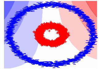
Figure 1 demonstrates the comparison of the decision boundaries between FM and SEFM on circles data, which is a nonlinear synthetic classification dataset in two-dimensional space. The blue points in the large outer circle belong to one class and the red points in the inner circle belong to the other class. As shown in sub-figure (a), the nonlinear decision boundary based on polynomial feature expansion produced by FM cannot capture the highly nonlinear pattern. SEFM (sub-figure (b)) produces the piecewise axis perpendicular decision boundary which works well on this data. The sub-figure (c) shows the decision boundary of our proposed method which also works very well on this nonlinear data but with much less memory cost compared with SEFM.
3 Methodology
3.1 Binarized Factorization Machines
Even though SEFM improves the model expressiveness capacity of FM and therefore achieves higher accuracy than FM on highly nonlinear datasets, SEFM increases the memory cost of FM by times since the model parameters are and where is times larger than the original data dimensionality . The high space complexity of SEFM will limit its applications in resource-constrained scenarios, such as model deployment on mobile phones or IoT devices.
To reduce the memory cost of SEFM, we propose to binarize the model parameter and . We approximate the full-precision and using binarized and and scaling parameters , . That is, and . The predicted value of our model will be
| (6) |
In our experiment, we show that using the scaling parameter and can get better accuracy than without using them. The objective of our proposed model can be formulated as
| (7) |
where in (7) denotes a convex loss function. Due to the non-smooth binary constraints, optimization of (7) is an NP-hard problem and it will need time to get the global optimal solution. Next, we will show how to optimize (7) efficiently using STE with Adagrad.
3.2 Learning Binary Model Parameters by Straight Through Estimator (STE)
In this section, we describe our proposed algorithm to solve (7) based on Straight Through Estimator (STE) (Bengio et al.,, 2013). STE is popularly used for training binary convolution neural networks (Alizadeh et al.,, 2018). The idea of STE is to learn a full-precision variable as the proxy of the binary variable during the training process. As in our proposed model, we introduce a full-precision as the proxy of binary in (7) and a full-precision as the proxy of binary in (7). Instead of directly learning binary variables and , we learn their full-precision proxy variables and . To estimate the binary variables and and scaling parameter , , we propose to minimize and .
Here we present our detailed derivation of estimating , and scaling parameter , based on the full-precision proxy variables and . The derivation follows the similar procedures of optimizing binary convolution neural networks (Rastegari et al.,, 2016). In the STE framework, we use SGD to update full-precision proxy variables and instead of , . We propose to get an optimal approximation for and by minimizing and .
Let us consider minimize first. By expanding the equation, it can be rewritten as
| (8) |
Since , will equals to a constant . The scaling parameter and is a known variable in (8). Therefore, to minimize (8) is equivalent to the following optimization problem,
| (9) |
It is straightforward to the optimal solution for (9), which is . To obtain the optimal solution for the scaling parameter , we take the derivative of (8) with respective to . It is . By setting it to 0, we will get . Since , the scaling parameter will be
| (10) |
By following the same procedure, we can also get the optimal and the optimal as
| (11) |
The optimal binary is obtained by , where sign() is the element-wise sign function which return 1 if the element is larger or equal than zero and return otherwise. Similarly, can be obtained by . Since the sign() function are not differentiable, STE estimates the gradients with respect to and as if the non-differentiable function sign() is not present. In other word, STE will simply estimate as . In practice, we also employ the gradient clipping as in (Hubara et al.,, 2016). Then, the gradient for the non-differentiable sign function is
| (12) |
Therefore, the gradient of (7) with respect to (i.e., the -th element in the proxy variable ) based on the -th data sample can be estimated as
| (13) |
Any convex loss function can be used in (13) and the gradient can be easily obtained for different loss function.
Similarly, the gradient of (7) with respect to (i.e., the -th element in ) based on the -th data sample can be estimated as
3.3 Updating the Proxy Variables by Adagrad
In our objective optimization problem (7), the feature representation after binning is very sparse since it is generated by applying one-hot encoding to each original feature. Also, the sparsity rate for different features in will be very different, as shown in Figure 2. Therefore, parameters associated with features with high sparsity rate will be updated less frequently than parameters associated with features with low sparsity rate in SGD. If we directly applied the standard SGD where the same learning rate is set for all parameters, it could be either too small for the parameters associated with features with high sparsity rate or too large for the parameters associated with features with low sparsity rate.
To address this issue, we propose to use Adagrad (Duchi et al.,, 2011) to update proxy variables and . Adagrad uses different learning rates for different model parameters and the learning rates can be adaptively adjusted during the training process. It has been shown that Adagrad can greatly improve the robustness of SGD (Ruder,, 2016). The basic intuition of Adagrad is to give low learning rates for parameters associated with features with low sparsity rate and to given high learning rates for parameters associated with features with high sparsity rate.
For a parameter (e.g., or ) in our model, based on the idea of Adagrad, we set the learning rate in the -th update to where equals the sum of squares of previously observed gradients up to time and is a small constant that prevents division by 0.
Therefore, for updating the -th element in , we can first obtain the gradient as in (13). Then, the updating rule for at the -th time will be
| (16) |
where aggregates sum of squares of previously observed gradients up to time . That is,
Similarly, for updating the -th parameter in , we first obtain the gradient as in (14). Then, the updating rule for at the -th time will be
| (17) |
where aggregates sum of squares of previously observed gradients with respect to up to time . That is,


As shown in (16) and (17), Adagrad adaptively adjusts the learning rate at each time step for each parameter in and based on their past gradients. In our experiment, we have shown that Adagrad can achieve lower training loss and is more robust than SGD.
| Method | Memory Cost (bits) |
|---|---|
| FM | 32 ( + ) |
| SEFM | 32 ( + ) |
| DFM | 32 + |
| Binarized FM | + |
| Dataset | Performance | Liblinear | FM | DFM | NFM | SEFM | Binarized FM |
|---|---|---|---|---|---|---|---|
| //#class | |||||||
| circles | accuracy (%) | 47.881.75 | 49.201.29 | 51.032.94 | 99.950.04 | 99.910.08 | 99.950.06 |
| 5,000/2/2 | prediction time (ms) | 0.3 | 2.0 | 2.2 | 39.3 | 1.6 | 1.6 |
| memory cost | 0.06 | 1 | 0.12 | 893 | 30 | 0.94 | |
| moons | accuracy (%) | 89.680.42 | 88.570.37 | 88.710.96 | 99.930.07 | 99.990.00 | 99.990.00 |
| 5,000/2/2 | prediction time (ms) | 0.3 | 2.7 | 2.8 | 92.7 | 1.8 | 1.2 |
| memory cost | 0.01 | 1 | 0.02 | 130 | 3.95 | 0.12 | |
| banana | accuracy (%) | 56.100.58 | 54.823.65 | 56.741.12 | 68.491.88 | 88.980.47 | 89.250.48 |
| 5,300/2/2 | prediction time (ms) | 0.3 | 1.7 | 2.0 | 132.2 | 1.3 | 1.8 |
| memory cost | 0.06 | 1 | 0.09 | 1849 | 30 | 3.66 | |
| breast-cancer | accuracy (%) | 95.020.94 | 94.730.64 | 95.221.26 | 96.910.74 | 95.510.94 | 96.200.64 |
| 683/10/2 | prediction time (ms) | 0.2 | 0.9 | 0.8 | 13.0 | 0.6 | 0.6 |
| memory cost | 0.06 | 1 | 0.12 | 300 | 30 | 3.58 | |
| segment | accuracy (%) | 91.521.03 | 91.981.60 | 90.511.09 | 88.170.87 | 94.230.82 | 94.750.82 |
| 2,310/19/7 | prediction time (ms) | 0.3 | 2.6 | 4.1 | 136.5 | 30.1 | 16.4 |
| memory cost | 0.06 | 1 | 0.18 | 484 | 19.4 | 2.37 | |
| pendigits | accuracy (%) | 93.120.36 | 94.260.61 | 95.740.45 | 94.290.15 | 97.380.12 | 97.560.16 |
| 10,992/16/10 | prediction time (ms) | 0.9 | 168.2 | 36.6 | 2,045.1 | 1,268.8 | 1,700.3 |
| memory cost | 0.01 | 1 | 0.04 | 53 | 10 | 0.31 | |
| ijcnn | accuracy (%) | 92.080.20 | 94.750.26 | 94.590.35 | 95.610.08 | 96.290.18 | 96.450.09 |
| 49,990/22/2 | prediction time (ms) | 8.9 | 158.3 | 193.7 | 651.2 | 125.7 | 229.2 |
| memory cost | 0.01 | 1 | 0.04 | 45 | 7.67 | 0.94 | |
| webspam | accuracy (%) | 92.710.04 | 95.490.72 | 95.210.15 | 97.530.12 | 98.110.13 | 97.790.08 |
| 350,000/254/2 | prediction time (ms) | 67.4 | 5,025.2 | 4,997.9 | 54,605.7 | 7,792.2 | 7,004.4 |
| memory cost | 0.01 | 1 | 0.04 | 2.06 | 30 | 0.94 |
3.4 Algorithm Implementation and Analysis
We summarize our proposed method in Algorithm 1. The step 1 obtains the new feature representation by applying one-hot encoding on each feature in input data which can be done in time (Lan and Geng,, 2019). The step 2 initializes the proxy variables , and , which are used for adjusting learning rate in Adagrad. From step 3 to 21, we update the proxy parameters and the binary parameters using STE with Adagrad. The time complexity for learning the binarized parameter is , where denotes the number of non-zero values in , is the low-rank parameter and is the number of passes over dataset . Empirically, the algorithm converge very fast and is a small number in our experiments.
3.5 Model Inference of Our Proposed Model
Similar to Lemma 3.1 in (Rendle,, 2010), the prediction score of our model for a given input can be written as
| (18) |
Since each element in is either 1 or , and where is the number of non-zero values in which will be equal to because of one-hot encoding. Also note that and are binary weights and is a sparse vector with nonzero values. The nonzero value in can only be 1. Therefore, the model inference as shown in (18) can be estimated by very efficiently only using addition and subtraction operations (without the need of multiplication operation). Also the arithmetic operations in (18) can be further replaced cheap XNOR and POPCOUNT bitwise operations (Rastegari et al.,, 2016).
4 Experiments
In this section, we compare our proposed method with other competing algorithms on eight datasets. The summary information of each dataset is given in the first column of Table 2. Among them, there are three synthetic datasets and five real-life datasets. These three synthetic datasets (i.e., circles, moons and banana) are widely used for evaluation nonlinear models. For the real-life datasets, three of them are binary classification and two of them are multi-class classification. One-vs-all strategy is used for multi-class classification.
In our experiments, we evaluate the performance of the following six different classification methods:
-
•
Liblinear: an efficient solver for linear support vector machine (Fan et al.,, 2008).
- •
-
•
DFM: Discrete Factorization Machines (Liu et al.,, 2018) which binarize the feature interaction parameters in FM. The DFM model focused on regression loss, and we extend it for classification loss.
-
•
NFM: Neural Factorization Machines (He and Chua,, 2017) which combines the FM with the neural networks.
-
•
SEFM: It improves expressive limitation of FM by one-hot encoding to each input features (Lan and Geng,, 2019).
-
•
Binarized FM: our proposed method.
4.1 Experimental Setting.
For each dataset, we randomly select 70% as training data and use the remaining 30% as test data. This procedure is repeated for 10 times and we report the average accuracy on test data. The low-rank parameter for FM, SEFM, DFM and Binarized FM is chosen from {16, 32, 64, 128}. The parameter (i.e., the number of bins) of SEFM and Binarized FM is chosen from {10, 20, 30, 40, 50}. The regularization parameter in Liblinear, FM, DFM and SEFM is chosen from . The optimal parameter combination is selected by 5-fold cross-validation on training data. The suggested settings are used in NFM, but for webspam, the hidden factor and the number of layers are both decreased to make it successfully run in our computing environment.


4.2 Experiment Results.
The accuracy, prediction time and memory cost of all six algorithms are reported in Table 2. Note that the memory cost of model parameters is normalized by the memory cost of standard FM. For example, 10x means the memory cost is 10 times larger than standard FM. The best accuracy for each dataset is in bold. The second best accuracy is in italic.
Accuracy. As shown in Table 2, both SEFM and our proposed method Binarized FM achieve higher accuracy than Liblinear, FM and DFM on all eight datasets. This is due to the fact that the expressiveness capacities of Liblinear, FM and DFM are smaller than SEFM and our proposed binarized FM. Overall, the linear classifier (i.e., Liblinear) gets the lowest accuracy, while FM and DFM get higher accuracy than the linear classifier. DFM is less accurate than FM because of binarizing of feature interaction model parameters. Our proposed method Binarized FM achieves comparable results with SEFM with much lower memory cost.
Memory cost. With regard to memory cost, Liblinear and DFM have much lower memory cost than FM, as Liblinear is a linear classifier being linear in the parameters and DFM binarize the 2-dimensional parameter of FM. As for our proposed method Binarized FM, which binarizes both the parameter and and transforms features by one-hot encoding, it has relatively lower memory cost on circles, moons, pendigits, ijcnn and webspam than FM and slightly higher memory costs on the other datasets. The memory costs of SEFM and NFM are much higher than FM and our proposed method on all of datasets.
We visually present the variation between memory cost and accuracy among four methods–FM, SEFM, DFM and Binarized FM on six different datasets as shown in Figure 3. It is clearly discovered that our proposed method Binarized FM can achieve higher accuracy than FM and DFM. With the same memory cost, Binarized FM has predominantly higher accuracy than FM. SEFM has the high accuracy and the highest memory cost, while the memory cost of our proposed method Binarized FM is obviously lower and its accuracy approaches that of SEFM.
The effect of scaling parameter and . The accuracy and prediction time of our algorithms with and without scaling parameter are reported in Table 3. After adding the scaling parameter and , our method achieves higher accuracy on most of datasets than without using them, especially on banana, segment, pendigits, ijcnn and webspam.
| Dataset | Performance | Without | With |
|---|---|---|---|
| //#class | scaling | scaling | |
| parameter | parameter | ||
| circles | accuracy(%) | 99.970.06 | 99.950.06 |
| 5,000/2/2 | prediction time | 1.5ms | 1.6ms |
| moons | accuracy(%) | 99.990.00 | 99.990.00 |
| 5,000/2/2 | prediction time | 1.2ms | 1.2ms |
| banana | accuracy(%) | 87.010.60 | 89.250.48 |
| 5,300/2/2 | prediction time | 1.5ms | 1.8ms |
| breast-cancer | accuracy(%) | 96.001.06 | 96.200.64 |
| 683/10/2 | prediction time | 0.8ms | 0.6ms |
| segment | accuracy(%) | 92.290.51 | 94.750.82 |
| 2,310/19/7 | prediction time | 17.5ms | 16.4ms |
| pendigits | accuracy(%) | 95.900.39 | 97.560.16 |
| 10,992/16/10 | prediction time | 1.5273s | 1.7003s |
| ijcnn | accuracy(%) | 95.130.20 | 96.450.09 |
| 49,990/22/2 | prediction time | 0.2037s | 0.2292s |
| webspam | accuracy(%) | 96.710.08 | 97.790.08 |
| 350,000/254/2 | prediction time | 7.1381s | 7.0044s |
Illustration of Decision Boundaries on Synthetic Datasets. We first illustrate that our proposed method can produce highly nonlinear decision boundary as SEFM on the synthetic datasets. We show the decision boundaries of FM, SEFM, DFM and our proposed binarized FM on moons and banana datasets in Figure 4. As shown in this figure, both FM and DFM can not capture the highly nonlinear pattern on these two datasets since they only used polynomial expansion on the original data to model the nonlinear relationship. SEFM and our proposed binarized FM can produce complex piecewise axis perpendicular decision boundary.


Comparison of the Convergence of Adagrad and SGD in Binarized FM. In addition to demonstrating the performance of our proposed method, we illustrate our training process by presenting the variation of training loss during iteration to prove our optimization method–Adagrad has more efficient performance than SGD. As shown in Figure 5, Adagrad reaches the lower training loss fast and gradually tend to converge.


5 Conclusion
In this paper, we propose a novel method Binarized FM that can reduce the memory cost of SEFM by binarizing the model parameters while maintaining comparable accuracy as SEFM. Since directly learning the binary model parameters is an NP-hard problem, we propose to use STE with Adagrad to efficiently learn the binary model parameters. We also provide a detailed analysis of our proposed method’s space and computational complexities for model inference and compare it with other competing methods. Our experimental results on eight datasets have clearly shown that our proposed method can get much better accuracy than FM while having similar memory cost and can achieve comparable accuracy with SEFM but with much less memory cost. We also demonstrate that learning model parameters by STE with Adagrad can converge very fast during the iteration of training the input dataset.
References
- Alizadeh et al., (2018) Alizadeh, M., Fernández-Marqués, J., Lane, N. D., and Gal, Y. (2018). An empirical study of binary neural networks’ optimisation.
- Bayer, (2016) Bayer, I. (2016). fastfm: A library for factorization machines. Journal of Machine Learning Research, 17(184):1–5.
- Bengio et al., (2013) Bengio, Y., Léonard, N., and Courville, A. (2013). Estimating or propagating gradients through stochastic neurons for conditional computation. arXiv preprint arXiv:1308.3432.
- Chang et al., (2010) Chang, Y.-W., Hsieh, C.-J., Chang, K.-W., Ringgaard, M., and Lin, C.-J. (2010). Training and testing low-degree polynomial data mappings via linear svm. Journal of Machine Learning Research, 11(4).
- Chen et al., (2019) Chen, X., Zheng, Y., Zhao, P., Jiang, Z., Ma, W., and Huang, J. (2019). A generalized locally linear factorization machine with supervised variational encoding. IEEE Transactions on Knowledge and Data Engineering, 32(6):1036–1049.
- Duchi et al., (2011) Duchi, J., Hazan, E., and Singer, Y. (2011). Adaptive subgradient methods for online learning and stochastic optimization. Journal of machine learning research, 12(7).
- Fan et al., (2008) Fan, R.-E., Chang, K.-W., Hsieh, C.-J., Wang, X.-R., and Lin, C.-J. (2008). Liblinear: A library for large linear classification. Journal of machine learning research, 9(Aug):1871–1874.
- Guo et al., (2017) Guo, H., Tang, R., Ye, Y., Li, Z., and He, X. (2017). Deepfm: a factorization-machine based neural network for ctr prediction. In Proceedings of the 26th International Joint Conference on Artificial Intelligence, pages 1725–1731.
- He and Chua, (2017) He, X. and Chua, T.-S. (2017). Neural factorization machines for sparse predictive analytics. In Proceedings of the 40th International ACM SIGIR conference on Research and Development in Information Retrieval, pages 355–364.
- Hubara et al., (2016) Hubara, I., Courbariaux, M., Soudry, D., El-Yaniv, R., and Bengio, Y. (2016). Binarized neural networks. In Advances in neural information processing systems, pages 4107–4115.
- Lan and Geng, (2019) Lan, L. and Geng, Y. (2019). Accurate and interpretable factorization machines. In Proceeding of the Thirty-Third AAAI Conference on Artificial Intelligence (AAAI), pages 4139–4146.
- Liu et al., (2017) Liu, C., Zhang, T., Zhao, P., Zhou, J., and Sun, J. (2017). Locally linear factorization machines. In Proceedings of the 26th International Joint Conference on Artificial Intelligence, pages 2294–2300. AAAI Press.
- Liu et al., (2018) Liu, H., He, X., Feng, F., Nie, L., Liu, R., and Zhang, H. (2018). Discrete factorization machines for fast feature-based recommendation. In Proceedings of the 27th International Joint Conference on Artificial Intelligence, pages 3449–3455.
- Rastegari et al., (2016) Rastegari, M., Ordonez, V., Redmon, J., and Farhadi, A. (2016). Xnor-net: Imagenet classification using binary convolutional neural networks. In European conference on computer vision, pages 525–542. Springer.
- Rendle, (2010) Rendle, S. (2010). Factorization machines. In IEEE 10th International Conference on Data Mining (ICDM), pages 995–1000.
- Ruder, (2016) Ruder, S. (2016). An overview of gradient descent optimization algorithms. arXiv preprint arXiv:1609.04747.
- Shen et al., (2017) Shen, F., Mu, Y., Yang, Y., Liu, W., Liu, L., Song, J., and Shen, H. T. (2017). Classification by retrieval: Binarizing data and classifiers. In Proceedings of the 40th international ACM SIGIR conference on research and development in information retrieval, pages 595–604.
- Xiao et al., (2017) Xiao, J., Ye, H., He, X., Zhang, H., Wu, F., and Chua, T.-S. (2017). Attentional factorization machines: learning the weight of feature interactions via attention networks. In Proceedings of the 26th International Joint Conference on Artificial Intelligence, pages 3119–3125.