Melting of generalized Wigner crystals in transition metal dichalcogenide heterobilayer Moiré systems
Abstract
Moiré superlattice systems such as transition metal dichalcogenide heterobilayers have garnered significant recent interest due to their promising utility as tunable solid state simulators. Recent experiments on a WSe2/WS2 heterobilayer detected incompressible charge ordered states that one can view as generalized Wigner crystals. The tunability of the hetero-TMD Moiré system presents an opportunity to study the rich set of possible phases upon melting these charge-ordered states. Here we use Monte Carlo simulations to study these intermediate phases in between incompressible charge-ordered states in the strong coupling limit. We find two distinct stripe solid states to be each preceded by distinct types of nematic states. In particular, we discover microscopic mechanisms that stabilize each of the nematic states, whose order parameter transforms as the two-dimensional representation of the Moiré lattice point group. Our results provide a testable experimental prediction of where both types of nematic occur, and elucidate the microscopic mechanism driving their formation.
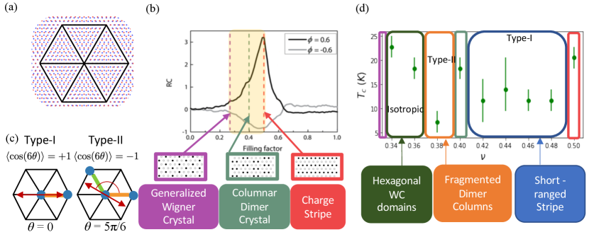
The promise of a highly tunable lattice system that can allow solid-state-based simulation of strong coupling physics Andrei et al. (2021) has largely driven the explosion of efforts studying Moiré superlattices. The transition metal dichalcogenide (TMD) heterobilayer Moiré systems with zero twist-angle (see Fig. 1(a)) and localized Wannier orbitals form a uniquely simple platform to explore phases driven by strong interactions Tang et al. (2020); Regan et al. (2020). Indeed, upon sweeping the density of electrons per Moiré unit cell, incompressible charge ordered states have been observed at various fractional fillings Regan et al. (2020); Xu et al. (2020); Li et al. (2021a). These charge orders can be viewed as a generalized Wigner crystalline state that reduces the symmetry of the underlying Moiré lattice, as they are driven by the long-range Coulomb interaction. The density controlled melting of Wigner crystals is expected to result in a rich hierarchy of intermediate phases Spivak and Kivelson (2004, 2006); Jamei et al. (2005). While a microscopic theoretical study of Wigner crystal melting is challenging due to the continuous spatial symmetry, the melting of generalized Wigner crystals is more amenable to a microscopic study due to the lattice. The observation of intermediate compressible states with optical anisotropy Jin et al. (2021) (see Fig. 1(b)) and the tunability beyond density Li et al. (2021b); Ghiotto et al. (2021) present a tantalizing possibility to study melting and the possible intermediate phases of the generalized Wigner crystals.
The underlying lattice in the generalized Wigner crystal reduces the continuous rotational symmetry to point group symmetry. Ref. Coppersmith et al. (1982) studied the melting of a -filled crystalline state on a triangular lattice in the context of Krypton adsorbed on Graphene. Based on the free energy costs of the domain walls and domain wall intersections, they reasoned that the generalized WC would first melt into a hexagonal liquid, and then crystallize into a stripe solid. From the modern perspectives of electronic liquid crystals Kivelson et al. (1998), one anticipates nematic fluid states in the vicinity of crystalline anisotropic states such as the stripe solid. Moreover, the point group symmetry of the triangular lattice relevant for hetero-TMD Moiré sytems further enriches the possibilities of the intermediate fluid phases. The triangular lattice admits two types of nematic states due to the nematic order parameter transforming as a 2-dimensional irreducible representation of the lattice point group Serre (2012); Fernandes and Venderbos (2020). The hetero-TMD Moiré systems present an excellent opportunity to study these intermediate liquid phases.
As the quantum melting of charge order is a notoriously difficult problem Kivelson et al. (2003), in this paper we will take advantage of the small bandwidth in hetero-TMD and use a strong coupling approach. We study Monte Carlo simulations inspired by hetero-TMD Moiré systems at and between commensurate charge ordered states. We analyze our results in terms of the structure factor and a nematic order parameter correlation function. In particular, we distinguish between the two possible types of nematic states illustrated in Fig. 1(c), one associated with the director aligned with a single majority bond orientation (which we dub type-I), and the other perpendicular to a single minority bond orientation (type-II). As shown in Fig. 1(d), we find the type-I nematic and type-II nematic to each robustly appear between 2/5 and 1/2 and 1/3 and 2/5 respectively. We conclude with a discussion.
As the orientation of the nematic director is defined within the angle range (Fig. 1(c)) we define the local nematic field using complex notation , where . In terms of this nematic order parameter field, the free energy density describing the isotropic-nematic transition in a trigonal system takes the following form Fernandes and Venderbos (2020); Venderbos and Fernandes (2018); Hecker and Schmalian (2018); Little et al. (2020):
| (1) |
The sign of the coefficient of the cubic term, , determines whether the system wants to be in a type-I nematic state () or type-II nematic state ().
We explore the phase diagram using classical Monte Carlo as a function of temperature and the number of particles per Moiré site . To emulate the experimental setup in refs. Xu et al. (2020); Jin et al. (2021); Li et al. (2021c); Regan et al. (2020), the Hamiltonian that we simulate describes the Coulomb interaction for electrons halfway between two dielectric gates a distance apart with dielectric constant :
| (2) |
Here, is the modified Bessel function of the second kind, is the Moiré lattice constant, and are the occupancies of lattice sites . As in refs. Xu et al. (2020); Jin et al. (2021), we take and , and we take as our unit of energy for simulation.
Because the interaction is long-ranged, simply simulating a system with periodic boundary conditions would result in ambiguous distance calculations. Thus, we simulate a formally infinite system that is constrained to be periodic in an rhombus. Particles interact both within and between copies of the system. The choice of an rhombus has the full symmetry of the triangular lattice as, when one considers the infinite system, the action of each element of the point group is a bijective map on the set of unique sites contained within the simulation cell. Thus we do not expect our choice of geometry to artificially promote rotational symmetry breaking. Moreover in each nematic state that we report, our simulations find configurations with each of the three possible director orientations for the relevant nematic type with equal probability. For Monte Carlo updates, we use arbitrary-range, single particle occupancy exchanges with standard Metropolis acceptance rules. However, the prevalence of short-range correlated structures leading to long autocorrelation times complicates our simulations, especially in the incompressible density region. To deal with this, we developed a cluster algorithm in the spirit of the well-known Wolff algorithm Wolff (1989) and the later geometric cluster algorithm Heringa and Blöte (1998). For more detail, see appendix A. We perform a cluster update after every 1000 single particle occupancy exchange updates.
At each point in phase space, we calculate the Monte Carlo average of the structure factor
| (3) |
to assess crystalline order. To assess the degree of rotational symmetry breaking, we also calculate the average of the nematic order parameter correlation function (per site) given by
| (4) |
where denotes Fourier momentum. At high temperatures, when , behaves as times the nematic susceptibility: . Generically we expect this to have some continuous behavior as a function of temperature. However, when the order parameter develops an expectation value in a nematic state, should acquire a constant, non-zero value. To determine the type of nematicity exhibited by nematic states, we also calculate , where, as in Fig. 1(c), type-I (type-II) nematic states have . For further details about the calculation of these quantities from our Monte Carlo simulation data, see appendix B. All results that we show are obtained from an system, except for exactly at since is not an integer. In all cases, we perform updates per site for equilibration at each temperature, and then updates per site for data collection.
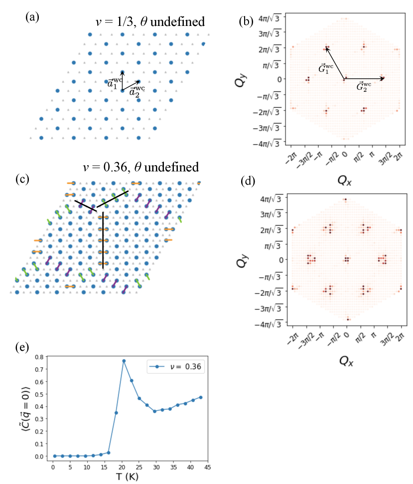
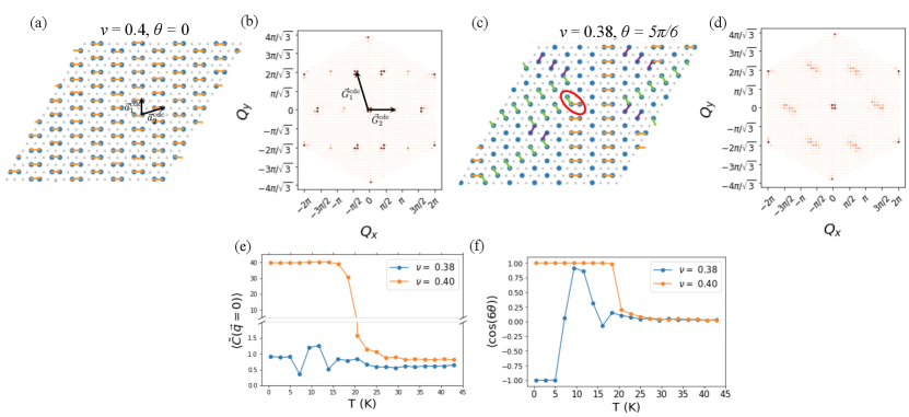
At , we find the isotropic generalized Wigner crystalline phase, shown in Fig. 2(a) for . This phase has lattice vectors and as indicated by the black arrows in Fig. 2(a). The structure factor shows well defined peaks at the reciprocal lattice vectors and associated with the crystalline state (Fig. 2(b)). Upon increasing the density, this crystalline state starts to melt, but it maintains an isotropic, compressible state to a certain filling. At small fillings away from the -state, as shown in Fig. 2(c), the extra particles form domain walls between the three different registries of the generalized WC state. Three domain walls are marked with black lines in Fig. 2(c). The domain walls meet at angles, reminiscent of what was found in ref. Coppersmith et al. (1982).
As in ref. Coppersmith et al. (1982), this domain wall structure is stable while the density of domain walls is dilute (and hence the domain walls are long) because energetics favor angles. Taking into account interactions up to fifth neighbor, the energy contributed to the Hamiltonian by the six particles in the three dimers composing the vertex is
| (5) |
while that of the particles composing three straight domain wall dimers is
| (6) |
where denotes the energy of two ’th neighbor particles. Using eq.( 2) it is easy to check that , and thus (at least to this order of interaction), it is energetically favorable to have -vertices, even at low temperatures. However, the densest possible hexagonal domain state consists of a close packing of -vertices, which has density . Thus, this state certainly cannot exist at densities . In Fig. 2(d), the structure factor of this compressible state is still dominated by the generalized WC, but with the domain size becoming finite, the superstructure peaks are broadened. Looking at the ensemble averaged nematic correlation function in Fig. 2(e) confirms that this state is isotropic as it drops to zero below the transition.
The state is dramatically different at . We have the charge stripe state shown in Fig. 3(a) with lattice vectors and . There are two degenerate charge stripe states whose lattice vectors are related by and rotations of . The structure factor in Fig. 3(b), averaged over configurations with the same orientation as the one shown in Fig. 3(a), contains peaks at the reciprocal lattice vectors and . As expected, . Diluting the -filled state, the stripes become shorter via the introduction of dislocations, as shown in Fig 3(c). The structure factor reflects the finite length of these stripe domains in the splitting of the stripe peak over the span of the stripe domain size scale. The peak at is split into two peaks separated by where is the average stripe domain size. The nematic correlation function reveals that, unlike the isotropic phases in Fig. 2(e), shows a sharp jump at to a finite value in Fig. 3(e). This indicates that these are nematic states. By examining in Fig. 3(f), we can see that both of these phases are type-I nematic.
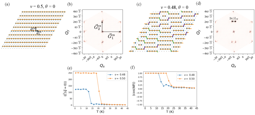
Upon further diluting, the system maintains the same type of anisotropy and forms the columnar dimer crystal state at , shown in Fig. 4(a) with director orientation . This is the limit of the shortest stripe length, evolving from . The state is a crystalline state with lattice vectors and . We mark the reciprocal lattice vectors and in the structure factor shown in Fig. 4(b). Note that the peak at is more intense than the one at . This is due to the form factor from the lattice basis. As we dilute further, the length of the columns get shorter as dimers get broken up. At lower densities, the columns do not extend over the entire system, so there are finite length segments of columns that can have different orientations as illustrated in Fig. 4(c). The broken pieces of dimers form short-range correlated domains of generalized WC. This is shown by the broad peaks in the structure factor in Fig. 4(d). This compressible state no longer has the mirror symmetries of the columnar state. It is still anisotropic as we can see from the nematic correlation function in Fig. 4(e). Interestingly, the columnar fragments intersect at angles, as well as angles, one of which is circled in red in fig. 4(c). While the intersections are isotropic, the intersections consist primarily of only two of the three possible nearest-neighbor bond orientations, and hence this state is a type-II nematic phase. We confirm this by observing that at low temperatures in Fig. 4(f). Thus we predict microscopic mechanism for the type-II nematic phase.
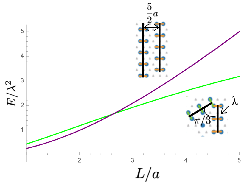
The nematic-II state in the region of is supported energetically. Upon increasing density beyond , columnar fragments have to either intersect also at or be parallel to each other. Since the distance between columnar fragments increases away from the intersection, we expect intersections to be favored. See appendix C for a schematic calculation demonstrating this. Such intersections involve two nearest-neighbor bond orientations, promoting a nematic-II state.
One could experimentally probe our predicted nematic states by performing optical measurements similar to those done at in ref. Jin et al. (2021). As one lowers the density from to we would anticipate a rotation of the nematic director and consequently a shift in the peaks of the measured optical anisotropy axis. In particular, as one decreases the density from between and , we predict that the measured anisotropy axis should have peaks along the nematic-I orientations . Below , when the director rotates into the nematic-II state, the peaks should be at . Finally, below when the system becomes isotropic, we expect that there should be no preferred anisotropy axis at all. For , one could also look for signatures of the hexagonal WC domain state using Umklapp spectroscopy experiments like those done in ref. Shimazaki et al. (2021). The short-range correlated nature of this state should show up as broadened Umklapp resonances around the generalized Wigner crystal lattice vectors.
In summary, we studied the electronic states of a system of strongly correlated electrons on a triangular lattice in the region particles per Moiré site. At , we find the charge stripe state. Upon dilution, the charge stripe state melts into a nematic-I short-ranged charge stripe state via the introduction of dislocations. Once the stripes become short enough, the columnar dimer crystal state emerges at . At even lower densities, the remaining columnar fragments space themselves out to lower their energy by intersecting at and angles, resulting in a nematic-II state. Below , the system can again lower its energy by using only columnar fragment intersections to form an isotropic, hexagonal network of domain walls between regions of the generalized Wigner crystal. Finally, at , the pure, isotropic generalized Wigner crystal state emerges. Our intermediate states were not only promoted by entropy, but we also found them to have lower energy compared to macroscopically phase separated states. Accordingly, we suspect that our proposed states are relevant for finite experimental temperatures where fluctuations due to entropy also play a role. We leave the determination of the classical ground state at as a subject of future work.
Studying the intermediate phases of melted density waves has been of interest since considerations of Krypton adsorbed on graphene Coppersmith et al. (1982). However, limitations in computational resources and experimental methods caused difficulties in probing the intermediate states. With advances in computing power and the advent of the TMD Moiré platform, however, detailed phase diagrams can now be predicted computationally and probed experimentally. Our work demonstrates this capacity to explore intermediate phases and the richness of the phase diagram one can obtain with a classical model, even without considering quantum effects. We found the striped phase predicted upon increasing density in ref. Coppersmith et al. (1982) refines into two distinct stripe crystal states neighboring two distinct types of nematics. In particular, we presented a microscopic mechanism for the formation of the nematic-II state via intersections between columnar fragments. As a subject of future work, it would be interesting to study the implications of our findings for the melting of WCs without a lattice potential, such as those recently observed in Zhou et al. (2021); Smoleński et al. (2021).
Acknowledgements: The authors acknowledge support by the NSF [Platform for the Accelerated Realization, Analysis, and Discovery of Interface Materials (PARADIM)] under cooperative agreement no. DMR-U638986. We would also like to thank Steven Kivelson, Kin-Fai Mak, Jie Shan, Sue Coppersmith, Ataç Imamoğlu, and Samuel Lederer for helpful discussions.
References
- Andrei et al. (2021) Eva Y. Andrei, Dmitri K. Efetov, Pablo Jarillo-Herrero, Allan H. MacDonald, Kin Fai Mak, T. Senthil, Emanuel Tutuc, Ali Yazdani, and Andrea F. Young, “The marvels of moiré materials,” Nature Reviews Materials 6, 201–206 (2021).
- Tang et al. (2020) Yanhao Tang, Lizhong Li, Tingxin Li, Yang Xu, Song Liu, Katayun Barmak, Kenji Watanabe, Takashi Taniguchi, Allan H. MacDonald, Jie Shan, and Kin Fai Mak, “Simulation of Hubbard model physics in WSe2/WS2 moirésuperlattices,” Nature 579, 353–358 (2020).
- Regan et al. (2020) Emma C. Regan, Danqing Wang, Chenhao Jin, M. Iqbal Bakti Utama, Beini Gao, Xin Wei, Sihan Zhao, Wenyu Zhao, Zuocheng Zhang, Kentaro Yumigeta, Mark Blei, Johan D. Carlström, Kenji Watanabe, Takashi Taniguchi, Sefaattin Tongay, Michael Crommie, Alex Zettl, and Feng Wang, “Mott and generalized Wigner crystal states in WSe2/WS2 moirésuperlattices,” Nature 579, 359–363 (2020).
- Xu et al. (2020) Yang Xu, Song Liu, Daniel A. Rhodes, Kenji Watanabe, Takashi Taniguchi, James Hone, Veit Elser, Kin Fai Mak, and Jie Shan, “Correlated insulating states at fractional fillings of moirésuperlattices,” Nature 587, 214–218 (2020).
- Li et al. (2021a) Hongyuan Li, Shaowei Li, Emma C. Regan, Danqing Wang, Wenyu Zhao, Salman Kahn, Kentaro Yumigeta, Mark Blei, Takashi Taniguchi, Kenji Watanabe, Sefaattin Tongay, Alex Zettl, Michael F. Crommie, and Feng Wang, “Imaging two-dimensional generalized Wigner crystals,” Nature 597, 650–654 (2021a).
- Spivak and Kivelson (2004) Boris Spivak and Steven A. Kivelson, “Phases intermediate between a two-dimensional electron liquid and Wigner crystal,” Phys. Rev. B 70, 155114 (2004).
- Spivak and Kivelson (2006) Boris Spivak and Steven A. Kivelson, “Transport in two dimensional electronic micro-emulsions,” Annals of Physics 321, 2071–2115 (2006).
- Jamei et al. (2005) Reza Jamei, Steven Kivelson, and Boris Spivak, “Universal Aspects of Coulomb-Frustrated Phase Separation,” Phys. Rev. Lett. 94, 056805 (2005).
- Jin et al. (2021) Chenhao Jin, Zui Tao, Tingxin Li, Yang Xu, Yanhao Tang, Jiacheng Zhu, Song Liu, Kenji Watanabe, Takashi Taniguchi, James C. Hone, Liang Fu, Jie Shan, and Kin Fai Mak, “Stripe phases in WSe2/WS2 moiré superlattices,” Nat. Mater. 20, 940–944 (2021).
- Li et al. (2021b) Tingxin Li, Shengwei Jiang, Lizhong Li, Yang Zhang, Kaifei Kang, Jiacheng Zhu, Kenji Watanabe, Takashi Taniguchi, Debanjan Chowdhury, Liang Fu, Jie Shan, and Kin Fai Mak, “Continuous Mott transition in semiconductor moiré superlattices,” Nature 597, 350–354 (2021b).
- Ghiotto et al. (2021) Augusto Ghiotto, En-Min Shih, Giancarlo S. S. G. Pereira, Daniel A. Rhodes, Bumho Kim, Jiawei Zang, Andrew J. Millis, Kenji Watanabe, Takashi Taniguchi, James C. Hone, Lei Wang, Cory R. Dean, and Abhay N. Pasupathy, “Quantum criticality in twisted transition metal dichalcogenides,” Nature 597, 345–349 (2021).
- Coppersmith et al. (1982) S. N. Coppersmith, Daniel S. Fisher, B. I. Halperin, P. A. Lee, and W. F. Brinkman, “Dislocations and the commensurate-incommensurate transition in two dimensions,” Phys. Rev. B 25, 349–363 (1982).
- Kivelson et al. (1998) S. A. Kivelson, E. Fradkin, and V. J. Emery, “Electronic liquid-crystal phases of a doped Mott insulator,” Nature 393, 550–553 (1998).
- Serre (2012) Jean-Pierre Serre, Linear Representations of Finite Groups (Springer Science & Business Media, 2012).
- Fernandes and Venderbos (2020) Rafael M. Fernandes and Jörn W. F. Venderbos, “Nematicity with a twist: Rotational symmetry breaking in a moiré superlattice,” Science Advances 6 (2020), 10.1126/sciadv.aba8834, https://advances.sciencemag.org/content/6/32/eaba8834.full.pdf .
- Kivelson et al. (2003) S. A. Kivelson, I. P. Bindloss, E. Fradkin, V. Oganesyan, J. M. Tranquada, A. Kapitulnik, and C. Howald, “How to detect fluctuating stripes in the high-temperature superconductors,” Rev. Mod. Phys. 75, 1201–1241 (2003).
- Venderbos and Fernandes (2018) Jörn W. F. Venderbos and Rafael M. Fernandes, “Correlations and electronic order in a two-orbital honeycomb lattice model for twisted bilayer graphene,” Phys. Rev. B 98, 245103 (2018).
- Hecker and Schmalian (2018) Matthias Hecker and Jörg Schmalian, “Vestigial nematic order and superconductivity in the doped topological insulator Cu x Bi2Se3,” npj Quant Mater 3, 26 (2018).
- Little et al. (2020) Arielle Little, Changmin Lee, Caolan John, Spencer Doyle, Eran Maniv, Nityan L. Nair, Wenqin Chen, Dylan Rees, Jörn W. F. Venderbos, Rafael M. Fernandes, James G. Analytis, and Joseph Orenstein, “Three-state nematicity in the triangular lattice antiferromagnet Fe1/3NbS2,” Nat. Mater. 19, 1062–1067 (2020).
- Li et al. (2021c) Hongyuan Li, Shaowei Li, Mit H. Naik, Jingxu Xie, Xinyu Li, Jiayin Wang, Emma Regan, Danqing Wang, Wenyu Zhao, Sihan Zhao, Salman Kahn, Kentaro Yumigeta, Mark Blei, Takashi Taniguchi, Kenji Watanabe, Sefaattin Tongay, Alex Zettl, Steven G. Louie, Feng Wang, and Michael F. Crommie, “Imaging moiréflat bands in three-dimensional reconstructed WSe2/WS2 superlattices,” Nature Materials (2021c), 10.1038/s41563-021-00923-6.
- Wolff (1989) Ulli Wolff, “Collective Monte Carlo Updating for Spin Systems,” Phys. Rev. Lett. 62, 361–364 (1989).
- Heringa and Blöte (1998) J. R. Heringa and H. W. J. Blöte, “Geometric cluster Monte Carlo simulation,” Phys. Rev. E 57, 4976–4978 (1998).
- Shimazaki et al. (2021) Yuya Shimazaki, Clemens Kuhlenkamp, Ido Schwartz, Tomasz Smoleński, Kenji Watanabe, Takashi Taniguchi, Martin Kroner, Richard Schmidt, Michael Knap, and Ataç Imamoğlu, “Optical Signatures of Periodic Charge Distribution in a Mott-like Correlated Insulator State,” Phys. Rev. X 11, 021027 (2021).
- Zhou et al. (2021) You Zhou, Jiho Sung, Elise Brutschea, Ilya Esterlis, Yao Wang, Giovanni Scuri, Ryan J. Gelly, Hoseok Heo, Takashi Taniguchi, Kenji Watanabe, Gergely Zaránd, Mikhail D. Lukin, Philip Kim, Eugene Demler, and Hongkun Park, “Bilayer Wigner crystals in a transition metal dichalcogenide heterostructure,” Nature 595, 48–52 (2021).
- Smoleński et al. (2021) Tomasz Smoleński, Pavel E. Dolgirev, Clemens Kuhlenkamp, Alexander Popert, Yuya Shimazaki, Patrick Back, Xiaobo Lu, Martin Kroner, Kenji Watanabe, Takashi Taniguchi, Ilya Esterlis, Eugene Demler, and Ataç Imamoğlu, “Signatures of Wigner crystal of electrons in a monolayer semiconductor,” Nature 595, 53–57 (2021).
Appendix A Appendix A: Cluster Algorithm for Monte Carlo Simulation
This appendix details the cluster algorithm we developed for our Monte Carlo simulations of the triangular Ising lattice gas with long range interactions. This algorithm is similar in spirit to the well-known Wolff algorithm Wolff (1989) and its later generalization: the so-called geometric cluster algorithm used to simulate the fixed magnetization ensemble of the nearest-neighbor Ising model Heringa and Blöte (1998). It is useful to consider the triangular lattice with sites as having its sites indexed by integer values . We define an injective map that takes an integer lattice site index and maps it to a real space coordinate. The precise action of this map depends on the details of the finite-size geometry. However, it will always return a linear combination of the triangular lattice vectors, i.e. with lattice unit vectors such that for some integer valued functions and where is the lattice constant.
One can view a particle configuration as a set specifying occupied sites of the lattice. The Lattice is occupied by Ising variables, and the occupancy function acts on a site index and configuration as
We are interested in the case of a fixed number of particles , i.e. the only valid particle configurations are those with cardinality .
We treat elements of the triangular lattice point group as maps which map lattice site indices to lattice site indices. Particle exchange is a map defined as
Note that preserves the cardinality of .
The Hamiltonian for the system is
where .
Algorithm:
-
1.
Fix a particle configuration , and initialize an empty set (the cluster)
-
2.
Choose an order-2 element, , of the lattice point group.
-
3.
Randomly choose a site , set and
-
4.
For each other site with and :
-
(a)
Calculate
The form of is chosen to ensure detailed balance (more detail in the next section).
-
(b)
With probability , set , , and record in a stack data structure
-
(a)
-
5.
Pop an element from the stack and repeat step with playing the role of
-
6.
Repeat step until the stack is empty and then return the updated particle configuration .
Proof of Detailed Balance:
To prove that this generates the correct equilibrium probability distribution (Boltzmann distribution), we need to show that the probability of a particle configuration moving to a configuration , , satisfies the detailed balance condition, i.e.
| (7) |
Observe that, for a move corresponding to a cluster , we can write where the first factor is the probability of forming the cluster containing the sites in and the second is the probability that no sites in are included in . Similarly, we write .
Because (1) is order-2 and a symmetry of and (2) only depends on lattice sites in , we have that .
By construction of the algorithm, we have (using standard probability rules) that
and
where in the last equation we have used the fact that for , . Thus we have that
| (8) |
where in the second equality we have used that is order-2 and a symmetry of the Hamiltonian. Note also the factor of , which is due to the fact that since and the sum double counts.
What remains is to show that the RHS of eq. 7 is the same as eq. 8. Using the fact that is order-2 and a symmetry of the Hamiltonian, we can write
It is then easy to see that the difference
This completes the proof and establishes that the algorithm defined above satisfies detailed balance.
A Note about Ergodicity:
Note that by choosing as an appropriate reflection, it is
possible to form a cluster consisting of a nearest neighbor particle exchange
with finite probability. Therefore, it is possible with finite probability
to get from any particle configuration to any other in the same way that
it is possible to realize any spin configuration in an Ising model via
a sequence of single spin flips. Thus we can see that this algorithm is
indeed ergodic.
Appendix B Appendix B: Calculation of nematic correlation function and orientation
To calculate the nematic order parameter expectation value in Monte Carlo, we write as
| (9) |
where the vectors point to the nearest neighbors of and is the occupation number of the site at . This is easy to calculate directly from a Monte Carlo configuration and average over the Markov chain. To calculate the orientation we use the fact that we can write the vector part of the nematic order parameter as . From this we can simply calculate and hence from the nematic order parameter and average it over the Markov chain.
Appendix C Appendix C: Energetics of intersection and parallel dimer column fragments
We can understand why the intersections are energetically preferred schematically by calculating the energy for two continuous, isolated wires of uniform line charge density interacting via eq. 2 as a function of wire length . We approximate the wires as being at the center of the dimer columns, and plot the results for parallel wires separated by in the purrple curve in Fig. S1. For a intersection with wires at the center of the dimers, the wires terminate with a separation of . We show the results for such wires in the green curve in Fig. S1. Indeed, the energy of the parallel wires exceeds that of the angled wires for sufficient .