Mechanical hysterons with tunable interactions of general sign
Abstract
Hysterons are elementary units of hysteresis that underlie many complex behaviors of non-equilibrium matter. Because models of interacting hysterons can describe disordered matter, this suggests that artificial systems could respond to mechanical inputs in precise and targeted ways. Specifying the properties of hysterons and their interactions could thus be a general method for realizing arbitrary non-equilibrium behaviors. Elastic structures including slender beams, creased sheets, and shells are clear candidates for artificial hysterons, but complete control of their interactions has seemed impractical or impossible. Here we report a mechanical hysteron composed of rigid bars and linear springs, which has controllable properties and tunable interactions of general sign that can be reciprocal or non-reciprocal. We derive a mapping from the system parameters to the hysteron properties, and we show how collective behaviors of multiple hysterons can be targeted by adjusting geometric parameters on the fly. By transforming an abstract hysteron model into a physical design platform, our work demonstrates a route toward designed materials that can sense, compute, and respond to their mechanical environment.
When an amorphous solid, a disordered magnet, or a crumpled sheet is subjected to an oscillating global drive, it navigates a complex pathway through a multitude of locally-stable states [1]. A powerful approach for understanding these systems has been to focus on the localized hysteretic rearrangements—hysterons—that arise within them [2, 3, 4, 5, 6, 7, 8, 9, 10, 11, 12]. In such models, each hysteron possesses a pair of thresholds and at which it switches between its two possible states, . More general models incorporate interactions between hysterons [13, 14, 15, 16], so that the switching thresholds depart from their “bare” values as follows:
| (1) |
where is a microstate that specifies the and the encode cooperative () or frustrated () interactions that may be non-reciprocal ().
In addition to offering a foothold for understanding disordered media, Eq. 1 suggests a design principle for a class of synthetic matter. If the thresholds and interactions can be designed, materials could be created with tailored responses to different mechanical environments. As the states are readily interpreted as bits, such materials are endowed with digital memory and the ability to perform computations [17]. Several mechanical metamaterials have been developed to this end, including origami bellows [18], corrugated sheets [19], buckled beams [20, 21], and biholar sheets [22, 23]. Yet, even in this realm where one has complete control over the material architecture, no system has been able to realize the full generality of Eq. 1.
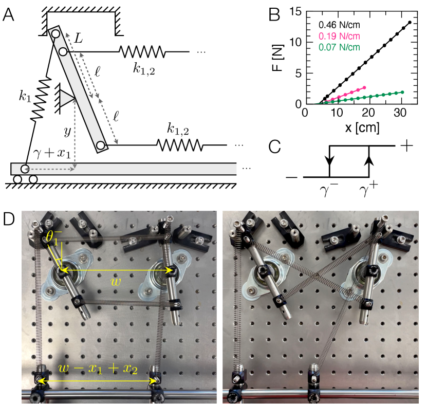
Here we show that it is possible to embody this abstract hysteron model in a physical system built from simple components: linear springs, rigid rods, and low-friction bearings (Fig. 1). We design interacting mechanical hysterons that allow: (i) tunable switching thresholds for each hysteron, (ii) tunable interactions between the hysterons that can be cooperative or frustrated, as well as reciprocal or non-reciprocal, and (iii) a tunable coupling to a global mechanical drive. We rationalize these results using an exact kinematic model, with a limiting behavior that maps the experimental parameters to the thresholds and interactions of Eq. 1. We then demonstrate the flexibility of the design by realizing a broad set of transition graphs for two interacting hysterons, as well as a “latching” behavior [24] that requires non-reciprocal interactions. Finally, we use larger collections of hysterons to accomplish more complex tasks: distinguishing between even and odd driving cycles [13] and counting the total number of driving cycles.
Our findings provide a general basis for mechanisms that navigate through precise sequences of states, e.g., in robotics [25]. More broadly, our results show that the size of the design space for hysteron-based materials, and the amount of control that can be wielded within it, is perhaps larger than previously thought. Our work thus identifies a vast potential for designed materials that inherently engage with memory [26], as their current state is a by-product of their driving history along with their overall design, which our platform now brings under the experimenter’s control.
Hysteron design.— Figure 1A illustrates the basic bistable unit in our system: a rigid bar that is free to rotate about a central pivot. The bar is corralled between two posts that restrict its angle to an interval, , with corresponding to vertical. We achieve precise, low-friction rotation using a radial steel ball bearing with the bearing grease removed. A spring of stiffness and rest length attaches to the bar a distance from the pivot; the other end of this spring attaches to a long steel shaft at a location along its length. The shaft translates freely along its axis via two linear bearings. The -position of this shaft, , will serve as the global mechanical drive. All springs used in the experiments behave linearly, which we verify by measuring their force-versus-displacement curves when pulling up on a known mass resting on an electronic balance (Fig. 1B).
Before investigating multiple coupled rotors, we consider the stability of a single rotor. Starting with the driving rod on the far left and gradually moving it to the right, the rotor begins in the () state where , but becomes unstable and jumps to the () state () when the line running through the spring passes the pivot point of the rod. This transition occurs when the horizontal displacement of the driving rod, , exceeds a threshold . Likewise, the rotor flips to when . The rotor is thus a hysteron: it is monostable outside the interval and it is bistable within (Fig. 1C).
To create interacting hysterons, we space two or more rotors a horizontal distance apart, and connect each rotor to the driving rod with its own spring of stiffness at an anchor point on the driving rod, measured from the horizontal position of hysteron when (Fig. 1D). We may then couple hysterons and together with additional springs of stiffness and rest length , mounted a distance from the pivot point (Fig. 1A). Uncrossed coupling springs create cooperative (ferromagnetic-like) interactions, which encourage two hysterons to occupy the same state, forming the composite states or more readily. Crossed springs create frustrated (antiferromagnetic-like) interactions, which encourage them to occupy the states or (Fig. 1D). More precisely, the switching thresholds for one hysteron become dependent on the state of the other, giving rise to an expanded set of thresholds. For example, will denote the threshold for hysteron 1 to switch to when hysteron 2 is in state . As we will show, these thresholds depend intimately on the geometric parameters in the setup and the properties of the springs.
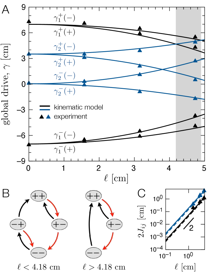
Tunable interactions.— The position where the coupling springs attach, , offers a convenient way to tune the interaction between the hysterons continuously. To demonstrate this control, we perform experiments on two hysterons with a cooperative interaction, where we fix all other system parameters and vary . We measure the switching thresholds by holding one rotor fixed in the or state, and quasistatically moving the driving rod until the other hysteron undergoes a transition. We measure the rod position with a precision of cm using a ruler affixed under the driving rod. Figure 2A shows the measured values of the eight transitions for this system, at four values of .
When , the spring has no lever arm to exert a torque on either rotor; in practice we remove the coupling springs for these measurements. Here there are only four distinct thresholds, due to the degeneracies . The particular order of the thresholds, , gives rise to a set of stable states and transitions that we may represent in a transition graph [5, 19] – a directed graph that shows the transitions out of each stable state under increasing or decreasing drive (Fig. 2B). For cm, the thresholds split into eight distinct values. Nevertheless, the same set of stable states and transitions manifest at this interaction strength, as well as for cm.
Increasing to cm, two pairs of thresholds switch their ordering: falls below , and falls below . The first switch does not change the transition graph for the system, but the second switch does. Starting in , the first transition upon increasing is to at . But this state is now unstable, as , meaning that hysteron 1 is above threshold to flip to as soon as hysteron 2 enters the state. This event is termed a “vertical avalanche” [15] and is denoted by the arrow from to in the second transition graph in Fig. 2B.
Kinematic model.— We can use torque balance to connect the system parameters to the switching thresholds observed in the experiment. First, we assume the system is in a stable state that specifies the . It is then straightforward to write down the Cartesian coordinates of each point where a coupling spring attaches to a rotor in terms of the variables , , and . Using the stiffness and rest lengths of the relevant coupling springs, one can then compute the torque of rotor on rotor . Similarly, one can compute the torque on rotor by its driving spring, denoted by . Hysteron will undergo a transition when the sum of the torques on it vanish 111To ensure this is an unstable equilibrium, it is necessary that , but also that the driving spring is sufficiently strong compared to any coupling springs that might disrupt this bistability.:
| (2) |
The that solve this equation are the switching thresholds, , wherein hysteron switches out of the state 222We do not presently have a precise condition on the parameters that would prohibit additional stable equilibria within the interval ..
Plugging in the experimental parameters for Fig. 2A, we compute these thresholds numerically and compare them with the data. The theory is in good agreement with the experiments. Moreover, the model allows us to anticipate precisely where the qualitative behaviors of the system will change, e.g., the change in the transition graph at (Fig. 2A,B). Another crossing of switching thresholds occurs at ; above this the avalanche from to occurs via the intermediate state , as now .
Mapping to general model at small rotor angles.— A closer study of Fig. 2A reveals some interesting facts about the system. First, the interactions may be non-reciprocal, meaning that the effect of hysteron 1 on hysteron 2 is not the same as the effect of hysteron 2 on hysteron 1. This can be seen by comparing the splitting of the blue curves for hysteron 2 as compared with the black curves for hysteron 1. Second, the mean of these pairs of thresholds, , may shift as a result of the interaction. In principle, one could understand these features of the system by examining the kinematic model, but in practice its nonlinear form conceals an intuitive understanding of these behaviors.
As we now show, we can build such an understanding by studying a limit where the rotor angles are small, . Moreover, this process will uncover a mapping from the metamaterial parameters to the model parameters of Eq. 1. To emphasize the core relationships in this mapping, we also specialize to the case where the two springs connecting a pair of rotors and have identical spring constants and rest lengths . We analyze the situation without these restrictions in the Appendix.
We begin by computing the torque of hysteron on , which under these conditions has a simple form: , where the geometric factor is defined by:
| (3) |
We further assume that the rest length of the driving spring is much less than . In this limit, the torque on rotor by its driving spring is: . We emphasize that this result is for small but general . To improve the accuracy of the expression at small , we replace the term with , which will recover the exact switching thresholds for the case of an uncoupled hysteron.
Taking these results together with Eq. 2 and defining and , we obtain an expression in the form of Eq. 1 with the following correspondences for the bare thresholds and the interactions, respectively:
| (4) | |||||
| (5) |
Note that the sum in Eq. 4 represents the shift of the bare threshold, , due to the presence of interactions, and although it closely resembles the interaction strength in Eq. 5, it is distinct from it. We also note that in this limit, the interactions evidently perturb the and the by the same amount, i.e., as in Eq. 1.
The non-reciprocity of the interaction can now immediately be seen, as depends on the angular interval but not on . The larger splitting of hysteron 2 in Fig. 2A is thus due to the larger angular interval of hysteron 1. To test this result quantitatively, Fig. 2C compares Eq. 5 with the value of from the full kinematic model and the experiments. The comparison shows that Eq. 5 captures the observed non-reciprocity, and that its dependence on is also in good agreement.
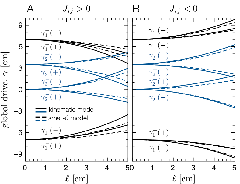
To test the small- model further, Fig. 3 compares the kinematic model with the small- model for a pair of hysterons with parallel springs (Fig. 3A) and crossed springs (Fig. 3B). The parameters are otherwise the same as in Fig. 2. The small- model captures the gross trends of all 8 switching thresholds in both configurations. In particular, the shift in is captured by the small- model, and is due to the last term in Eq. 4, which measures the difference between the mean rotor angle and the current rotor angle [recall that the () transition is out of the () state and vice versa]. This shift is the most apparent in the thresholds for hysteron 1 in Fig. 3, as that rotor is bounded by larger angles. In general, the pair and the pair shift in opposite directions, with the sign of the shift set by .
Finally, we note that the thresholds and interactions in Eqs. 4 and 5 are independent of . This means that one can couple together hysterons that are not adjacent, while maintaining the same design space for interactions. We also note that Eqs. 4 and 5 are readily adapted to heterogeneous or , which can be used to tune the coupling to the global drive or the relative pairwise interactions in larger systems. We make use of these features later on.
Targeting specific transition graphs.— The above results suggest that our mechanical hysterons should be able to produce many of the behaviors of the general hysteron model of Eq. 1. To develop a better sense of this presumed generality, and to see whether there are experimental limitations that hamper it, we begin by targeting different transition graphs for two coupled hysterons. As we do so, we also investigate a parallel question: To what extent can different functionalities be accessed while changing only a small number of system parameters?
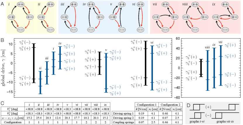
To this end, we start by demonstrating four distinct transition graphs in a sequence where we alter only the mounting position of driving spring 2, thereby changing only . Supplementary Movie 1 shows this sequence of behaviors, which correspond to transition graphs - in Fig. 4A. The experimental parameters are tabulated in Fig. 4C.
To understand how the system moves between these four transition graphs, we plug these parameters into the kinematic model, calculate the switching thresholds, and plot them in Fig. 4B. The switching thresholds of hysteron 1 are constant throughout this sequence, as they depend on the state of hysteron 2 but not its driving. The thresholds for hysteron 2 move in concert without changing their spacing, as changing shifts each threshold by . Careful inspection of the switching thresholds in Fig. 4B shows that they indeed produce graphs - in Fig. 4A, faithful to the experiment.
Next, we access transition graph by decreasing , increasing , and changing (Supplementary Movie 2). We access transition graph by setting = and changing once again (Supplementary Movie 3). This exhausts all possible transition graphs for two hysterons with cooperative interactions [15].
Three additional transition graphs can be obtained by using frustrated interactions [15]; they are graphs - in Fig. 4A. Supplementary Movie 4 shows how we can realize these graphs in the experiment while varying only to navigate between them. All three graphs feature at least one “horizontal avalanches”. To understand how they occur, start in the state in graph . The corresponding thresholds in Fig. 4B show that upon increasing , hysteron 2 switches first, as . Now in the state, the next event is at into . But this state is not stable, as this is below , which brings the system immediately to . An analogous process underlies each of the avalanches in graphs -.
Among these graphs, perhaps the most exotic is , which navigates the sequence: , , , under unidirectional driving. This behavior constitutes a 2-bit analog-to-digital converter [15]. We now describe the process used to target this transition graph, to illustrate how behaviors may be rationally designed in our system. First, we need a strong coupling between the global drive and hysteron 1, so that it is at small and at large . We also need a strong frustrated interaction between hysterons 1 and 2 to navigate the avalanches. In particular, the interaction of hysteron 1 on hysteron 2 must open up a central interval, where the state of hysteron 2 depends only on the current state of hysteron 1. Figure 4D illustrates this condition, and an examination of graphs - in Fig. 4 shows that they satisfy it. We target this condition by selecting a large and a sufficiently large ; we find that the same used in the other designs works here too. Finally, a weak coupling of hysteron 2 to the global drive enables a transition into the state at large and into at small . These considerations lead to a tentative design for the spring constants: . Here we use N/cm and N/cm, which we found to suffice.
Two additional transition graphs are possible for “mixed” interactions, where the signs of and differ [15]. We do not see a way to realize such interactions in our system.
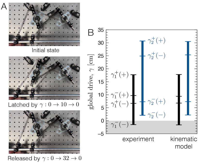
Latching.— The ability to manifest non-reciprocal frustrated interactions in this system allows one to access a behavior termed “latching”. This behavior was proposed by Lindeman et al. [24] to explain how amorphous solids form multiple memories of asymmetric driving. Here we demonstrate it with our mechanical hysterons in Fig. 5A and Supplementary Movie 5. Starting in the state at , we drive the system to cm, which puts the hysterons in the state. This state remains stable as we return back to ; hysteron 1 is now “latched” in the state. A larger driving amplitude to cm and back to releases hysteron 1 back to via a sequence of intermediate states: . This behavior necessarily violates return-point memory [29, 30, 26], which would stipulate that the same state would recur each time the driving returns to its common endpoint, .
Lindeman et al. [24] showed how latching is tied to the ordering of the switching thresholds. They found that latching requires:
| (6a) | ||||
| (6b) | ||||
We now show how we translate this ordering into a concrete design in our mechanical system. We start by noting that Eq. 6a implies: , which we rewrite as: . We obtain this non-reciprocal frustrated interaction by confining hysteron 1 to a smaller angular interval than hysteron 2 and coupling them together with crossed springs following Eq. 5. Next, we note that adjusting moves all thresholds for hysteron 2 in concert without altering their spacing. We thus move until and . Then, we fulfill by moving and together by equal amounts until those thresholds straddle . Finally, turns out to be satisfied already through the larger angular interval of hysteron 2.
Figure 5B shows the switching thresholds as measured in our experimental realization of latching, using the parameters in the caption. The ordering of thresholds indeed follow Eq. 6. Plugging the experimental parameters into the kinematic model, we obtain the second set of bars, which are in good agreement with the experiment and follow the same ordering.
Our mechanical system allows one to latch and release the hysterons in another way, shown in Supplementary Movie 6. Holding the driving rod fixed at , the left rotor can be flipped between the by hand, and it is stable in either state when the right rotor is . From the state , flipping the right rotor to immediately releases the left rotor to , returning the system to upon letting go.
Counting modulo 2.— More sophisticated functions can be realized with more hysterons. Here we target a multiperiodic response that was obtained for simulated hysterons [13, 14, 16]. We start with a design from one of those studies [13], where four hysterons are coupled as in Fig. 6A. When cyclic driving of unit amplitude is applied [31], these parameters produce the steady state drawn with black and red arrows in Fig. 6B, which we determine using the open-source hysteron software package [31]. The sequence of states takes two driving cycles to traverse. These interacting hysterons thus perform a basic computation: discriminating between even and odd numbers of driving cycles, i.e., counting modulo 2.
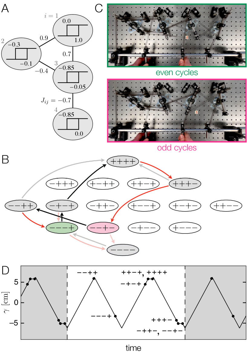
Investigating this pathway in Fig. 6B further, we can see that it features two avalanches ( and ), as well as a pair of “scrambled” transitions: and , meaning that they are not consistent with a state-independent ordering of the switching fields [19, 15]. To see this, note that these transitions imply that when , and that when . The presence of either scrambling or avalanches is known to be necessary, but not sufficient, for a multiperiodic response [15].
To reproduce this complex response in the lab, we start by translating the sign and approximate strength of the interactions into a choice of springs and their mounting points on the rotors, which controls the magnitude of the interaction via the product . One pair of springs spans a longer distance from rotor 1 to rotor 3; we attach a length of steel wire to extend the reach of these springs while staying within their linear response. We then set the for each hysteron to reflect its relative amount of hysteresis in the design. To ensure a repeatable minimum and maximum for the driving, we mount the two linear bearings that hold the driving rod at locations where they will collide with the outermost clamps that support springs 1 and 4, and we use these contacts as the turning points.
The mounting positions , the angular intervals , the coupling positions , and the two endpoints of the driving offer a total of 14 continuous degrees of freedom. On top of this, we also allow ourselves to mount some of the springs within a pair at unequal . To target the sequence of states in Fig. 6B, we drive the system to observe its behavior and then adjust one or more of these degrees of freedom to try to obtain more of the desired sequence. This iterative process eventually produced the configuration shown in Fig. 6C; its behavior under cyclic driving is shown in Supplementary Movie 7. To show the resulting steady state, we measure the value of where each transition occurs, and we plot the sequence of states as a function of time in Fig. 6D. The sequence matches that of Fig. 6B, it takes two periods to traverse, and it repeats indefinitely, as desired.
There is one subtle difference in the pathways: The experiment navigates the downward avalanche via the unstable intermediate state , whereas the design in Fig. 6A passes through instead. We found that we could match the experiment by changing the bare threshold for the top hysteron in Fig. 6A from to .
Counting to .— As a final demonstration of computing with mechanical hysterons, Fig. 7 and Supplementary Movie 8 show an accumulator, which counts the number of driving cycles applied to it. A mechanical metamaterial was recently designed with this function [32], using a train of carefully designed elastic beams that make and break contact under cyclic compression. Our design is based on an antiferromagnetic chain, here a series of hysterons with uniform frustrated interactions. We stagger the points where the springs attach to the driving rod, which alternatingly raises and lowers the values of and for each hysteron. In particular, we set , , and , where , although other values can also work. This design breaks the degeneracy of the two ground states so that has a higher energy than .
Starting in the higher-energy ground state, cycling the system at constant amplitude drives a domain wall down the chain, irreversibly flipping one hysteron each half cycle. These transitions occur because a hysteron at the domain wall experiences two interactions that cancel, allowing it to change state upon the influence of the global drive. The location of the domain wall thus encodes the number of driving cycles; hysterons can record this number up to . Once the domain wall reaches the end of the chain, the configuration is stable to further driving.
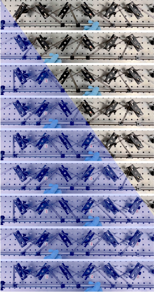
The basic idea of this design can be verified on a computer [31] by applying cyclic driving of any fixed amplitude , setting thresholds for the odd hysterons and for the even hysterons (where ), and setting nearest-neighbor interactions of strength . The thresholds for hysteron 1 should be raised by to allow a domain wall to nucleate there.
More precisely, our accumulator design detects cycles of intermediate amplitude. A small-amplitude cycle that stays within the interval will not change the state, and a large-amplitude cycle that overpowers the frustrated interactions can send the system to its final absorbing state. In our idealized example, the system counts cycles of any amplitude between and .
Discussion.— Here we have demonstrated a design for mechanical hysterons with continuously tunable thresholds and interactions, whose states can be controlled manually or by coupling to an external mechanical drive. Recent work has demonstrated other mechanical designs that can count modulo two [33], count driving cycles up to [32], or encode an analog mechanical input into a binary string [34]. Although those systems use bistable mechanical elements, each one uses a different strategy to navigate the pathways between its states. In contrast, we have presented a general platform that can be reconfigured to perform all of the above functions, plus a latching behavior that was recently identified in hysteron simulations [24]. Crucial to this versatility was the realization of cooperative and frustrated interactions that can be reciprocal or non-reciprocal.
One principle of our approach was to use nonlinearities sparingly, so that the behaviors of the system could be rationalized as simply as possible. We used linear springs and nearly-frictionless bearings in the experiment, and our analysis using small rotor angles and an affine relationship between torque and the global drive was able to capture the essential behaviors of two interacting hysterons (Fig. 3). Other designs for interacting mechanical hysterons are also being proposed; Shohat and van Hecke [35] used theory and simulations to explore two-dimensional networks of bilinear hysterons as a route to exotic pathways, including mixed interactions and multiperiodic cycles. Understanding what are the general constraints on and for any realizable metamaterial is an open question.
Designing the response of larger collections of mechanical hysterons presents another set of challenges. Although we report an exact kinematic model and a mapping to switching thresholds and interactions for small rotor angles, in practice we worked at relatively large rotor angles and proceeded through a combination of physical reasoning and trial-and-error. This approach might not work for larger hysteron machines. As an alternative, our kinematic model can provide the basis for computational inverse design methods, which could generate sets of parameters for a particular desired behavior. Another possibility for targeting behaviors in large systems is through supervised learning [36], which was recently implemented in experiments on spring networks [37]. Our system offers a wealth of possible learning degrees of freedom, as there are numerous geometric parameters that can be tuned continuously to affect the switching thresholds, including , , , and . Understanding whether this approach can be used achieve a specific transition graph or a desired response under cyclic drive could be a fertile direction for future work.
The focus of this work has been developing a mechanical hysteron with general interactions (Figs. 1-3), understanding these interactions (Eqs. 3-5), and probing their versatility through a series of targeted behaviors (Figs. 4-7). Some of these behaviors are readily interpreted as basic computations on mechanical inputs, like the accumulator that counts cycles of intermediate amplitude (Fig. 7). Yet, such computation is not limited to a small set of particular designs – rather, it is a general feature of collections of interacting hysterons. This can be realized by interpreting the transition graphs as finite-state machines (FSMs), through the selection of an initial state and an accept state and the choice of an alphabet of driving protocols, as described recently by Liu et al. [21]. For instance, the latching mechanism has a natural two-character alphabet of as S (set) and as R (reset). If the initial and accepting states are both , this FSM accepts the empty string and any string ending in R. The computational power of FSMs, paired with the existence of general mechanical hysterons that we have established here, suggests that there is a large, untapped potential for designed materials that can sense, compute, and respond to their mechanical environment.
Acknowledgements.
I thank Nathan Keim for suggesting how to apply a global drive, for providing the parameters used in Fig. 6A, and for many fruitful discussions. I thank Vidyesh Anisetti, Eadin Block, Christian Santangelo, and Jennifer Schwarz for contributing to early hysteron designs, and I thank Martin van Hecke, Nathan Keim, Chloe Lindeman, and Dor Shohat for comments on the manuscript. This work was initiated at the Aspen Center for Physics, which is supported by National Science Foundation grant PHY-2210452.Appendix A Appendix
Rotor hysteron construction.— We construct each rotor hysterons from two ”-diameter optical posts attached in a T configuration, which we mount in a radial steel ball bearing affixed to an optical table. We remove the bearing grease to further lower their friction to rotation. We use steel extension springs to couple the rotors to one another and to a 1/2”-diameter steel shaft that is mounted in two linear bearings. This 72”-long rod translates freely along the horizontal direction and provides the global mechanical drive, . We define as the horizontal displacement of this rod in centimeters, which we measure with a precision of cm via a ruler affixed under the rod.
Spring stiffnesses.— We measure the spring stiffnesses from force-versus-displacement data that we obtain by anchoring the springs to a known mass on an electronic balance, and recording the force on the balance as the top of the spring is extended and then retracted (Fig. 1B). These measurements show that the springs behave linearly over the range of extensions used in the experiments.
Torques for general coupling.— Here we derive expressions for the torques in the small- model, in the general case where the two springs connecting hysterons and are not necessarily paired with equal spring constants or rest lengths, and where they may not have symmetrical mounting positions. We begin by considering a single coupling spring of stiffness and rest length that mounts to rotors and at positions and from the fulcrums of the rotors, respectively, where the signs of , indicate the side of the fulcrum where they attach. In the limit of small , this coupling spring exerts a torque on hysteron 1 equal to:
| (7) |
where is the length of the spring when . With this result, it is straightforward to write down the net torque on rotor 1 for the general case where a second spring of stiffness and rest length is mounted at distinct positions and . The expression will in general depend on the properties and mounting positions of both springs, and will contain terms proportional to , , and , for both unprimed and primed .
Pairing the springs as in Fig. 1D with and greatly simplifies the interaction. Mounting the springs in a “parallel” configuration, , we obtain:
| (8) |
where the dependence on has vanished, and the dependence is on alone.
Mounting instead in a “crossed” configuration, , we obtain:
| (9) |
Specializing to simplifies this expression to:
| (10) |
which is equal and opposite to Eq. 8.
References
- Paulsen and Keim [2024] J. D. Paulsen and N. C. Keim, Mechanical memories in solids, from disorder to design, Annual Review of Condensed Matter Physics 16 (2024).
- Preisach [1935] F. Preisach, Über die magnetische nachwirkung, Zeitschrift für physik 94, 277 (1935).
- Falk and Langer [2011] M. L. Falk and J. Langer, Deformation and failure of amorphous, solidlike materials, Annual Review of Condensed Matter Physics 2, 353 (2011).
- Keim and Arratia [2014] N. C. Keim and P. E. Arratia, Mechanical and microscopic properties of the reversible plastic regime in a 2d jammed material, Phys. Rev. Lett. 112, 028302 (2014).
- Mungan et al. [2019] M. Mungan, S. Sastry, K. Dahmen, and I. Regev, Networks and hierarchies: How amorphous materials learn to remember, Phys. Rev. Lett. 123, 178002 (2019).
- Mungan and Terzi [2019] M. Mungan and M. M. Terzi, The structure of state transition graphs in systems with return point memory: I. general theory, Annales Henri Poincaré 20, 2819 (2019).
- Terzi and Mungan [2020] M. M. Terzi and M. Mungan, State transition graph of the preisach model and the role of return-point memory, Phys. Rev. E 102, 012122 (2020).
- Keim et al. [2020] N. C. Keim, J. Hass, B. Kroger, and D. Wieker, Global memory from local hysteresis in an amorphous solid, Phys. Rev. Res. 2, 012004 (2020).
- Keim and Medina [2022] N. C. Keim and D. Medina, Mechanical annealing and memories in a disordered solid, Science Advances 8, eabo1614 (2022).
- Shohat et al. [2023] D. Shohat, Y. Friedman, and Y. Lahini, Logarithmic aging via instability cascades in disordered systems, Nature Physics 19, 1890 (2023).
- Muhaxheri and Santangelo [2024] G. Muhaxheri and C. D. Santangelo, Bifurcations of inflating balloons and interacting hysterons, Phys. Rev. E 110, 024209 (2024).
- Martínez-Calvo et al. [2024] A. Martínez-Calvo, M. D. Biviano, A. H. Christensen, E. Katifori, K. H. Jensen, and M. Ruiz-García, The fluidic memristor as a collective phenomenon in elastohydrodynamic networks, Nature Communications 15, 3121 (2024).
- Keim and Paulsen [2021] N. C. Keim and J. D. Paulsen, Multiperiodic orbits from interacting soft spots in cyclically sheared amorphous solids, Science Advances 7, eabg7685 (2021).
- Lindeman and Nagel [2021] C. W. Lindeman and S. R. Nagel, Multiple memory formation in glassy landscapes, Science Advances 7, eabg7133 (2021).
- van Hecke [2021] M. van Hecke, Profusion of transition pathways for interacting hysterons, Phys. Rev. E 104, 054608 (2021).
- Szulc et al. [2022] A. Szulc, M. Mungan, and I. Regev, Cooperative effects driving the multi-periodic dynamics of cyclically sheared amorphous solids, The Journal of Chemical Physics 156, 164506 (2022).
- Yasuda et al. [2021] H. Yasuda, P. R. Buskohl, A. Gillman, T. D. Murphey, S. Stepney, R. A. Vaia, and J. R. Raney, Mechanical computing, Nature 598, 39 (2021).
- Jules et al. [2022] T. Jules, A. Reid, K. E. Daniels, M. Mungan, and F. Lechenault, Delicate memory structure of origami switches, Phys. Rev. Res. 4, 013128 (2022).
- Bense and van Hecke [2021] H. Bense and M. van Hecke, Complex pathways and memory in compressed corrugated sheets, Proceedings of the National Academy of Sciences 118, e2111436118 (2021).
- Sirote-Katz et al. [2024] C. Sirote-Katz, D. Shohat, C. Merrigan, Y. Lahini, C. Nisoli, and Y. Shokef, Emergent disorder and mechanical memory in periodic metamaterials, Nature Communications 15, 4008 (2024).
- Liu et al. [2024] J. Liu, M. Teunisse, G. Korovin, I. R. Vermaire, L. Jin, H. Bense, and M. van Hecke, Controlled pathways and sequential information processing in serially coupled mechanical hysterons, Proceedings of the National Academy of Sciences 121, e2308414121 (2024).
- Ding and van Hecke [2022] J. Ding and M. van Hecke, Sequential snapping and pathways in a mechanical metamaterial, The Journal of Chemical Physics 156, 204902 (2022).
- El Elmi and Pasini [2024] A. El Elmi and D. Pasini, Tunable sequential pathways through spatial partitioning and frustration tuning in soft metamaterials, Soft Matter 20, 1186 (2024).
- Lindeman et al. [2023] C. W. Lindeman, T. R. Jalowiec, and N. C. Keim, Isolating the enhanced memory of a glassy system (2023), arXiv:2306.07177 [cond-mat.soft] .
- Kamp et al. [2024] L. M. Kamp, M. Zanaty, A. Zareei, B. Gorissen, R. J. Wood, and K. Bertoldi, Reprogrammable sequencing for physically intelligent under-actuated robots (2024), arXiv:2409.03737 [cs.RO] .
- Keim et al. [2019] N. C. Keim, J. D. Paulsen, Z. Zeravcic, S. Sastry, and S. R. Nagel, Memory formation in matter, Rev. Mod. Phys. 91, 035002 (2019).
- Note [1] To ensure this is an unstable equilibrium, it is necessary that , but also that the driving spring is sufficiently strong compared to any coupling springs that might disrupt this bistability.
- Note [2] We do not presently have a precise condition on the parameters that would prohibit additional stable equilibria within the interval .
- Barker et al. [1983] J. A. Barker, D. E. Schreiber, B. G. Huth, and D. H. Everett, Magnetic hysteresis and minor loops: models and experiments, Proceedings of the Royal Society of London. A. Mathematical and Physical Sciences 386, 251 (1983).
- Sethna et al. [1993] J. P. Sethna, K. Dahmen, S. Kartha, J. A. Krumhansl, B. W. Roberts, and J. D. Shore, Hysteresis and hierarchies: Dynamics of disorder-driven first-order phase transformations, Phys. Rev. Lett. 70, 3347 (1993).
- Keim and Paulsen [2020] N. C. Keim and J. D. Paulsen, hysteron 0.1, https://github.com/nkeim/hysteron (2020).
- Kwakernaak and van Hecke [2023] L. J. Kwakernaak and M. van Hecke, Counting and sequential information processing in mechanical metamaterials, Phys. Rev. Lett. 130, 268204 (2023).
- ten Wolde and Farhadi [2024] M. A. ten Wolde and D. Farhadi, A single-input state-switching building block harnessing internal instabilities, Mechanism and Machine Theory 196, 105626 (2024).
- Hyatt and Harne [2023] L. P. Hyatt and R. L. Harne, Programming metastable transition sequences in digital mechanical materials, Extreme Mechanics Letters 59, 101975 (2023).
- Shohat and van Hecke [2024] D. Shohat and M. van Hecke, Geometric control and memory in networks of bistable elements (2024), arXiv:2409.07804 [cond-mat.soft] .
- Stern and Murugan [2023] M. Stern and A. Murugan, Learning without neurons in physical systems, Annual Review of Condensed Matter Physics 14, 417 (2023).
- Altman et al. [2024] L. E. Altman, M. Stern, A. J. Liu, and D. J. Durian, Experimental demonstration of coupled learning in elastic networks, Phys. Rev. Appl. 22, 024053 (2024).