Measuring quantum geometric tensor of non-Abelian system in superconducting circuits

Introduction.— Topology played a very important role in physics research in the last few decades nakahara2018geometry , including the areas of high energy physics and condensed matter physics PhysRevD.12.3845 ; WU1976365 ; RevModPhys.82.3045 ; RevModPhys.83.1057 ; goldman_light_2014 ; RevModPhys.90.015001 ; zhang_topological_2018 ; RevModPhys.91.015006 ; buluta_quantum_2009 ; bliokh_quantum_2015 . One of the most important quantities of topology is the quantum geometric tensor (QGT) provost_riemannian_1980 ; PhysRevLett.99.095701 ; PhysRevB.81.245129 , of which an imaginary part is the Berry curvature, which is closely related to many physical phenomena such as the Aharonov-Bohm phase PhysRev.115.485 and topological orders in condensed matter PhysRevB.44.2664 ; RevModPhys.89.041004 . The QGT can be used to classify various topological materials. Furthermore, the geometric phase is applied in the study of quantum computation and information ZANARDI199994 ; PhysRevA.61.010305 ; Bohm_gometric_phase_2003 , and it holds the promise to improve the performance of quantum gates due to its immunity to local fluctuations PhysRevLett.91.187902 ; PhysRevA.72.020301 ; PhysRevLett.102.030404 ; PhysRevA.96.052316 . The real part of the QGT, called the quantum metric tensor, characterizes the distance between states in a Hilbert space, which is closely related to quantum fluctuations PhysRevD.23.357 ; PhysRevLett.72.3439 . In the recent period of time, it has attracted interest of researchers in quantum phase transitions PhysRevE.74.031123 ; PhysRevLett.99.100603 ; sachdev_2011 ; carollo_geometry_2020 and quantum information theory PhysRevE.86.031137 . Both theoretical and experimental research has been conducted. For instance, similar to the well-known Chern number that characterizes the topological properties of the Dirac monopole noauthor_quantised_nodate ; RevModPhys.82.1959 ; ray_observation_2014 , the topological invariants of the tensor monopole are related to the geometric metric tensor PhysRevLett.121.170401 . The four-dimensional matter predicted by theory has been simulated in superconducting circuits PhysRevLett.126.017702 and NV-center chen2021synthetic , while its quantum phase transition is well characterized by the metric tensor PhysRevLett.121.170401 .

Compared to that of the Abelian quantum system, the quantum geometric tensor in the non-Abelian system has more complex mathematical structures and embodies more physics phenomena, including the four-dimensional Hall effect zhang2001four . The topological order of the non-Abelian quantum systems can be extracted from the tensor, revealing the relationship between the physics phenomena and topological properties. For instance, the second Chern number, as the topological invariant of the Yang monopole, is theoretically and experimentally studied yang_generalization_1978 ; sugawa_second_2018 ; PhysRevLett.117.015301 ; weisbrich_second_2021 . Furthermore, the Wilczek-Zee connection, which leads to the Holonomic properties in the generated system, allows the geometric gate to be widely used in quantum circuits PhysRevLett.52.2111 ; Duan_Geometric_2001 ; sugawa_wilson_2021 ; RevModPhys.80.1083 . This subject is extensively and thoroughly studied for the optimization of quantum gates sjoqvist_non_adiabatic_2012 ; PhysRevLett.109.170501 ; PhysRevLett.102.070502 ; PhysRevLett.95.130501 .

Therefore, measuring the generalized non-Abelian quantum geometric tensor has both theoretical and practical significance. However, detecting the geometric tensor of a complex system is tricky in practice. For an Abelian system, some approaches have been proposed, including modulation of Hamiltonian with sudden quench and periodic drivings PhysRevB.97.201117 ; PhysRevLett.122.210401 ; 10.1093/nsr/nwz193 . These routines have been realized in various systems such as superconducting circuits PhysRevLett.122.210401 and NV-center 10.1093/nsr/nwz193 . For a non-Abelian system, several theoretical detection schemes have been proposed PhysRevResearch.3.033122 , but there is still a lack of experimental demonstration.

In this work, we construct a non-Abelian system in four-qubit superconducting circuits. Using longitudinal parametric modulation PhysRevApplied.6.064007 ; Matthew_2018 ; PhysRevApplied.13.064012 , we demonstrate that the quantum geometric tensor, which depends on the geometry defined by a set of parameters, can be extracted by using geometric Rabi oscillations that are realized by periodically driving the system under a single parameter or under two parameters PhysRevB.97.201117 ; PhysRevResearch.3.033122 . We implement this protocol to simulate the Bernevig-Hughes-Zhang model and reveal its physics feature such as Z2 symmetry from the extracted topological invariant. The good agreement between experimental data and theoretical prediction confirms the validity of our approach.

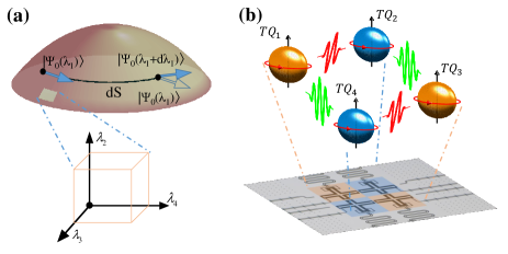
QGT in Non-Abelian systems.— We consider an $N$-band Hamiltonian with $n$-degeneracy dimensions, which can be written as $H_{0}(\lambda)=\sum_{\sigma=0}^{N}E_{\sigma}\sum_{i=1}^{n}|\psi_{i}^{\sigma}(\lambda)\rangle\langle\psi_{i}^{\sigma}(\lambda)|$ with a set of dimensionless parameters $\lambda=(\lambda_{1},\lambda_{2},\dots)$, while $|\psi_{i}^{0}(\lambda)\rangle$ is the ground state. Without loss of generality, we choose $N=1$ and $n=2$, so the dimension of the simulated Hamiltonian is four. Similar to that of the Abelian system, the geometric tensor can be derived from the distance between two nearby states in a Hilbert space, which is defined as $dS:=\left\||\Psi_{0}(\lambda_{1}+d\lambda_{1})\rangle-|\Psi_{0}(\lambda_{1})\rangle\right\|$, as illustrated in Fig. 1. Here $|\Psi_{0}(\lambda)\rangle=\sum_{i=1}^{n}|\psi_{i}^{0}(\lambda)\rangle$. The matrix element of the QGT PhysRevB.81.245129 can be found as

where $\partial_{\lambda_{\mu,\nu}}\equiv\partial/\partial\lambda_{\mu,\nu}$ and $\mathcal{P}(\lambda)$ stands for the projection operator, defined as $\mathcal{P}(\lambda)=\sum_{i=1}^{n}|\psi_{i}^{0}(\lambda)\rangle\langle\psi_{i}^{0}(\lambda)|$. Notice that the QGT is a complex matrix, of which the real and imaginary parts are the Riemannian metric and Berry curvature respectively: $g^{\mu\nu}=(Q^{\mu\nu}+[Q^{\mu\nu}]^{\dagger})/2$, and $F^{\mu\nu}=i(Q^{\mu\nu}-[Q^{\mu\nu}]^{\dagger})$.

To measure the QGT of the degenerate system, we construct the Hamiltonian $H_{0}$ and detect the interference oscillation with periodic weak parametric modulation PhysRevResearch.3.033122 . The values of the metric tensor and Berry curvature can be extracted from the measured Rabi frequencies. In this routine, the QGT elements are obtained with one- and two-parameter modulation, respectively. With the modulating amplitude $A$ and the frequency $\omega$ satisfy $A\ll\omega$ PhysRevB.97.201117 ; PhysRevResearch.3.033122 , the corresponding Hamiltonians expanded to first order are $H_{0}(\lambda)+h_{1}(\lambda_{\mu})$ or $H_{0}(\lambda)+h_{2}(\lambda_{\mu},\lambda_{\nu})$. Here $h_{1}(\lambda_{\mu})=\frac{2A}{\omega}\cos{(\omega t+\phi_{\mu})}\partial_{\lambda_{\mu}}H_{0}(\lambda)$ and $h_{2}(\lambda_{\mu},\lambda_{\nu})=\frac{2A}{\omega}[\cos{(\omega t+\phi_{\mu})}\partial_{\lambda_{\mu}}H_{0}(\lambda)+\cos{(\omega t+\phi_{\nu})}\partial_{\lambda_{\nu}}H_{0}(\lambda)]$.

To simplify the experimental scheme and improve measurement fidelity, we rotate the Hamiltonian with a unitary transformation, so the coupling terms become zero supplementary3 . In the modified Hamiltonian, the values of $Q^{\mu\nu}_{ij}$ can be extracted from the oscillation frequencies of the new eigenstates PhysRevResearch.3.033122 . The relation between the value $Q_{QGT}$ and the Rabi oscillation is

for one- and two-parameter modulation $Q_{QGT}$ equals $Q_{jj}^{\nu\nu}$ and $Q_{jj}^{\mu\mu}+Q_{jj}^{\nu\nu}+e^{-i\delta\phi}Q_{jj}^{\mu\nu}+e^{i\delta\phi}Q_{jj}^{\nu\mu}$ respectively. Here, $\delta\phi=\phi_{\nu}-\phi_{\mu}$ is the phase difference between the two periodic modulation pulses, $\Delta$ is the detuning between the gap of eigenenergy levels and the driving frequency $\omega$.

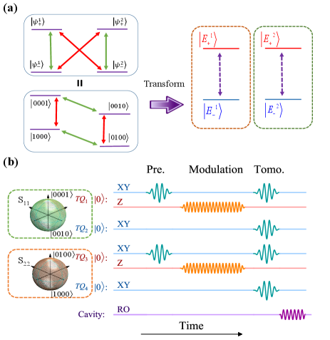
Build non-Abelian system.— The Hamiltonian constructed by four qubits can be written as $H_{s}=\sum_{k}\omega_{k}a^{\dagger}_{k}a_{k}+\frac{\alpha_{k}}{2}a^{\dagger}_{k}a^{\dagger}_{k}a_{k}a_{k}+\sum_{kl}J_{kl}(a_{k}+a_{k}^{\dagger})(a_{l}+a_{l}^{\dagger})$ with indices $k\in\{1,\,2,\,3,\,4\}$ and $kl\in\{12,\,23,\,34,\,41\}$ to mark qubits. Here, $a_{k}$ ($a^{\dagger}_{k}$) is the annihilation (creation) operator and $J_{kl}$ is the nearest-neighbor coupling strength, while $\alpha_{k}$ denotes the anharmonicity of the $k$-th transmon, of which the frequency in the lowest two levels is labeled as $\omega_{k}$ supplementary1 . To realize the desired degenerate Hamiltonian $H_{0}(\lambda)$, whose level structure can be equivalent to a diamond shape as shown in the right panel of Fig. 2(a), we simultaneously introduce the longitudinal parametric modulation pulses $\omega_{m}(t)=\bar{\omega}_{m}+\omega^{T}_{m1}\cos{(2\pi f_{m1}t+\beta_{m1})}+\omega^{T}_{m2}\cos{(2\pi f_{m2}t+{\beta}_{m2})}$ by applying flux pulses to the tunable qubit $QT_{m}$ supplementary2 . $\bar{\omega}_{m}$ is the mean frequency of $TQ_{m}$ during the longitudinal parametric modulation, $\omega^{T}_{mi}$, $f_{mi}$ and $\beta_{mi}$ is the amplitude, frequency and phase of the applied longitudinal pulse. The two-tune pulses of parametric modulation realize the diamond-shape couplings as illustrated in Fig. 1(b). In this approach the parameters of each coupling term can be freely adjusted, making that the general Non-Abelian Hamiltonian as shown in Fig. 2(a) can be directly realized in the Hilbert space spanned by $\{|0001\rangle,\,|0010\rangle,\,|0100\rangle,\,|1000\rangle\}$ supplementary2 .

Experimental results.— In practice, we detect the specific metrics to study the topological properties of physical models, here we constructed the Bernevig-Hughes-Zhang (BHZ) model as an example to demonstrate this scheme bernevig_quantum_2006 ; PhysRevLett.127.136802 ; supplementary3 . The BHZ model is closely related to the spin-Hall effect, which can be characterized by the spin Chern numbers. The Hamiltonian is

where $B_{x}=H_{xy}\sin{k_{x}},B_{y}=H_{xy}\sin{k_{y}},B_{z}=M-2H_{z}(2-\cos{k_{x}}-\cos{k_{y}})$. The momentum $k_{x},\,k_{y}$ belong to $[-\pi,\pi]$, while the parameters $H_{xy}$, $H_{z}$, and $B_{g}$ depend on the quantum well geometry, $M$ is related to the phase transition. In our superconducting circuit we can realize this BHZ Hamiltonian, which is a non-Abelian form in a four-dimensional parameter space. Its entire components of the QGT can be obtained by our approach supplementary4 , while it is not necessary in practice. The BHZ model is equivalent to two copies of the Haldane Model PhysRevLett.61.2015 ; PhysRevLett.127.136802 , which can be mapped to the Hilbert space of two degenerate systems. Therefore, the original Hamiltonian can be deformed to the individual degenerate subspace by a unitary transformation as shown in Fig. 2(a). The parametric modulation in experiment can be simplified as $\omega_{1}(t)=\bar{\omega}_{1}+\omega^{T}_{1}\cos{(2\pi f_{1}t+\varphi)}$ and $\omega_{3}(t)=\bar{\omega}_{3}+\omega^{T}_{3}\cos{(2\pi f_{3}t-\varphi)}$, leading that the system Hamiltonian in spherical coordinate can be written as supplementary2

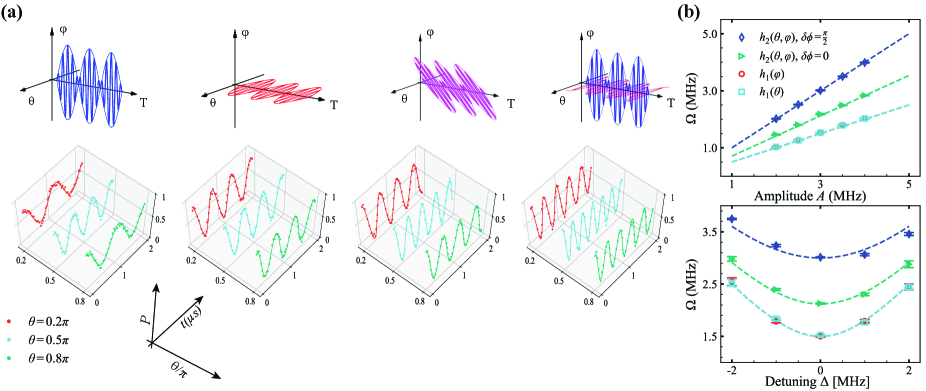
where $\Omega_{0}=\sqrt{\Omega^{2}+\Delta^{2}}$. Here $\Omega$ is the Rabi oscillation frequency in Eq. (2), with $\Omega=|J_{12}\mathcal{J}_{1}(\frac{\omega_{1}^{T}}{2\pi f_{1}})|=|J_{34}\mathcal{J}_{1}(\frac{\omega_{3}^{T}}{2\pi f_{3}})|$. $\mathcal{J}_{1}$ denotes the first kind 1st-order Bessel function. The spherical coordinate $\theta=\arctan({\Omega}/{\Delta})$. The QGT measurement, which contains initial state preparation, parametric modulation, and quantum state tomography, is demonstrated on four qubits by modulating the controlling parameters $\theta$ and $\varphi$.

To obtain the complete quantum metric of the manifold, we need to execute the procedure by preparing different initial states throughout the entire Hilbert space. To improve measurement fidelity, we use a unitary transformation to rotate the frame axis. The eigenstates of the initial Hamiltonian remain at $|0001\rangle$ and $|0100\rangle$ PhysRevLett.122.210401 , making the modulation pulse significantly simplified. With this routine, the weak periodic driving term $h_{1}(\lambda_{\mu})$ and $h_{2}(\lambda_{\mu},\lambda_{\nu})$ can be realized by accurately designing the frequency and amplitude of the flux pulses supplementary2 . For instance, in the measurement of $g^{\varphi\varphi}_{11}$, The parameter ${\varphi}$ in the modulated pulse simplified as $2A/\omega\cos(\omega t)$ with $A/2\pi=3$ MHz and $\omega/2\pi=13$ MHz. Fig. 3 shows the pulse schemes and measured Rabi patterns, with ${\theta}=0.2\pi$, $0.5\pi$ and $0.8\pi$, respectively. Similarly, the Rabi patterns of the other QGT terms ($g^{\theta\theta}_{11}$, $g^{\varphi\theta}_{11}$, and $F^{\varphi\theta}_{11}$) can also be obtained. Furthermore, we can verify the relationship between the QGT and the parameters of the periodic weak field in Eq. (2). As shown in Fig. 3(b), we vary the amplitude $A$ and detuning $\Delta$ as a double-check. The data demonstrated in the figure are measured at ${\theta}=0.5\pi$. Based on Eq. (2), in the top panel of Fig. 3(b), there is a linear relationship between $A$ and $\Omega$ if $\Delta/2\pi=0\,\rm{MHz}$, so the values of the QGT can be extracted from the experimental results, in the bottom panel of Fig. 3(b), by setting $A/2\pi=3\,\rm{MHz}$, the relationship between $\Delta$ and $\Omega$ also agrees well with the predictions (dashed lines). Note that $h_{1}(\theta)$ is almost identical to $h_{1}(\varphi)$. With this modulating protocol, we can extract the QGT of the simulating Hamiltonian, revealing the corresponding geometric properties. As shown in Fig. 4(a), The experimental $Q_{\mu\nu}$ are in good agreement with theoretical predictions, which are

It is worth noting that the Morris-Shore (MS) transformation used in our scheme reduces the parameter dimension, hence the complete components of the original geometric tensor are obtained by repeating this approach with different unitary transformation supplementary4 .

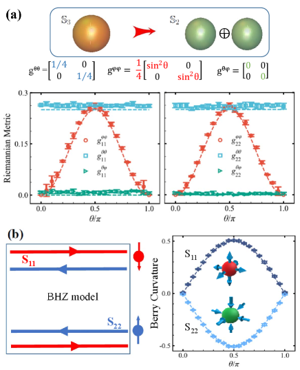
Furthermore, we study the topological invariant in the BHZ model, which is the spin Chern number. The spin up and down charge carriers correspond to the individual subspace $\mathcal{S}_{11}$ and $\mathcal{S}_{22}$ we constructed, of which the corresponding topological invariant is the first Chern number $\mathcal{C_{\pm}}$. Since the manifold is covered by three dimensional sphere surface $\mathbb{S}_{2}$, in spherical coordinates the Chern number of individual subspace can be written as

The relation $\sqrt{\rm{det}\,g}=\frac{1}{2}|F_{\theta\phi}|$ PhysRevLett.121.170401 ; zhang2021revealing ; PhysRevB.104.195133 ; mera_relating_2022 ensures that we can obtain the Chern number from the metric tensor $g^{\varphi\varphi}_{11(22)}$, $g^{\theta\theta}_{11(22)}$, $g^{\theta\varphi}_{11(22)}$ and Berry curvature $F^{\theta\varphi}_{11(22)}$ we measured, respectively. The accumulated values of the subspace $\mathcal{S}_{11}$ and $\mathcal{S}_{22}$ extracted from the Berry curvature are $\mathcal{C_{+}}=1.019\pm 0.005$ and $\mathcal{C_{-}}=-1.003\pm 0.010$, which correspond to the positive and negative topological charges respectively, as illustrated in Fig. 4(b). The spin Chern number is obtained as $\mathcal{C}_{scn}=(\mathcal{C}_{+}-\mathcal{C}_{-})/2=1.011\pm 0.005$ while $\mathcal{C}_{+}+\mathcal{C}_{-}=0.016\pm 0.013$ due to the time-reversal symmetry, indicating the Z2 symmetry of the Bernevig-Hughes-Zhang model PhysRevLett.95.146802 ; PhysRevLett.95.226801 ; PhysRevLett.95.136602 ; PhysRevLett.97.036808 ; sheng_spin_2013 . Therefore, the topological properties of BHZ model can be explored directly with our approach.

Conclusions.— In this article, we have demonstrated the simulation of a non-Abelian system in superconducting circuits. Using periodic driving, we measure the geometric tensor of this quantum system. In addition, we extract the topological invariant from the measured metric tensor and the Berry curvature, respectively, proving the feasibility and validity of our routine. Furthermore, our scheme is universal and can be extended to quantum simulations of other models.

Acknowledgement.— This work was supported by the Key R&D Program of Guangdong Province (Grant No. 2018B030326001), NSFC (Grants No. 11474152, No. 12074179, No. U21A20436, and No. 61521001), NSF of Jiangsu Province (Grant No. BE2021015-1).

References

- (1) M. Nakahara. Geometry, topology and physics. CRC press (2018).
- (2) T. T. Wu and C. N. Yang, Phys. Rev. D 12 3845, (1975).
- (3) T. T. Wu and C. N. Yang, Nucl. Phys. B 107 365, (1976).
- (4) M. Z. Hasan and C. L. Kane, Rev. Mod. Phys. 82 3045, (2010).
- (5) X.-L. Qi and S.-C. Zhang, Rev. Mod. Phys. 83 1057, (2011).
- (6) N. Goldman, G. Juzeliūnas, P. Öhberg, and I. B. Spielman, Rep. Prog. Phys. 77 126401, (2014).
- (7) N. P. Armitage, E. J. Mele, and A. Vishwanath, Rev. Mod. Phys. 90 015001, (2018).
- (8) D.-W. Zhang, Y.-Q. Zhu, Y. X. Zhao, H. Yan, and S.-L. Zhu, Adv. Phys. 67 253, (2018).
- (9) T. Ozawa, H. M. Price, A. Amo, N. Goldman, M. Hafezi, L. Lu, M. C. Rechtsman, D. Schuster, J. Simon, O. Zilberberg, and I. Carusotto, Rev. Mod. Phys. 91 015006, (2019).
- (10) I. Buluta and F. Nori, Science 326 108, (2009).
- (11) K. Y. Bliokh, D. Smirnova, and F. Nori, Science 348 1448, (2015).
- (12) J. P. Provost and G. Vallee, Commun. Math. Phys. 76 289, (1980).
- (13) L. Campos Venuti and P. Zanardi, Phys. Rev. Lett. 99 095701, (2007).
- (14) Y.-Q. Ma, S. Chen, H. Fan, and W.-M. Liu, Phys. Rev. B 81 245129, (2010).
- (15) Y. Aharonov and D. Bohm, Phys. Rev. 115 485, (1959).
- (16) X. G. Wen, Phys. Rev. B 44 2664, (1991).
- (17) X.-G. Wen, Rev. Mod. Phys. 89 041004, (2017).
- (18) P. Zanardi and M. Rasetti, Phys. Lett. A 264 94, (1999).
- (19) J. Pachos, P. Zanardi, and M. Rasetti, Phys. Rev. A 61 010305(R), (1999).
- (20) A. Bohm, A. Mostafazadeh, H. Koizumi, Q. Niu, and J. Zwanziger. The Geometric Phase in Quantum Systems: Foundations, Mathematical Concepts, and Applications in Molecular and Condensed Matter Physics (2003).
- (21) S.-L. Zhu and Z. D. Wang, Phys. Rev. Lett. 91 187902, (2003).
- (22) S.-L. Zhu and P. Zanardi, Phys. Rev. A 72 020301(R), (2005).
- (23) S. Filipp, J. Klepp, Y. Hasegawa, C. Plonka-Spehr, U. Schmidt, P. Geltenbort, and H. Rauch, Phys. Rev. Lett. 102 030404, (2009).
- (24) P. Z. Zhao, X.-D. Cui, G. F. Xu, E. Sjöqvist, and D. M. Tong, Phys. Rev. A 96 052316, (2017).
- (25) W. K. Wootters, Phys. Rev. D 23 357, (1981).
- (26) S. L. Braunstein and C. M. Caves, Phys. Rev. Lett. 72 3439, (1994).
- (27) P. Zanardi and N. Paunković, Phys. Rev. E 74 031123, (2006).
- (28) P. Zanardi, P. Giorda, and M. Cozzini, Phys. Rev. Lett. 99 100603, (2007).
- (29) S. Sachdev. Quantum Phase Transitions. Cambridge University Press, 2 edition (2011).
- (30) A. Carollo, D. Valenti, and B. Spagnolo, Phys. Rep. 838 1, (2020).
- (31) A. Dey, S. Mahapatra, P. Roy, and T. Sarkar, Phys. Rev. E 86 031137, (2012).
- (32) P. A. M. Dirac, Proc. R. Soc. Lond. A 133 60.
- (33) D. Xiao, M.-C. Chang, and Q. Niu, Rev. Mod. Phys. 82 1959, (2010).
- (34) M. W. Ray, E. Ruokokoski, S. Kandel, M. Möttönen, and D. S. Hall, Nature 505 657, (2014).
- (35) G. Palumbo and N. Goldman, Phys. Rev. Lett. 121 170401, (2018).
- (36) X. Tan, D.-W. Zhang, W. Zheng, X. Yang, S. Song, Z. Han, Y. Dong, Z. Wang, D. Lan, H. Yan, S.-L. Zhu, and Y. Yu, Phys. Rev. Lett. 126 017702, (2021).
- (37) M. Chen, C. Li, G. Palumbo, Y.-Q. Zhu, N. Goldman, and P. Cappellaro, Science 375 1017, (2022).
- (38) S.-C. Zhang and J. Hu, Science 294 823, (2001).
- (39) C. N. Yang, J. Math. Phys. 19 10, (1978).
- (40) S. Sugawa, F. Salces-Carcoba, A. R. Perry, Y. Yue, and I. B. Spielman, Science 360 1429, (2018).
- (41) M. Kolodrubetz, Phys. Rev. Lett. 117 015301, (2016).
- (42) H. Weisbrich, R. Klees, G. Rastelli, and W. Belzig, PRX Quantum 2 010310, (2021).
- (43) F. Wilczek and A. Zee, Phys. Rev. Lett. 52 2111, (1984).
- (44) L.-M. Duan, J. I. Cirac, and P. Zoller, Science 292 1695, (2001).
- (45) S. Sugawa, F. Salces-Carcoba, Y. Yue, A. Putra, and I. B. Spielman, npj Quantum Inform. 7 144, (2021).
- (46) C. Nayak, S. H. Simon, A. Stern, M. Freedman, and S. Das Sarma, Rev. Mod. Phys. 80 1083, (2008).
- (47) E. Sjöqvist, D. M. Tong, L. Mauritz Andersson, B. Hessmo, M. Johansson, and K. Singh, New J. Phys. 14 103035, (2012).
- (48) G. F. Xu, J. Zhang, D. M. Tong, E. Sjöqvist, and L. C. Kwek, Phys. Rev. Lett. 109 170501, (2012).
- (49) O. Oreshkov, T. A. Brun, and D. A. Lidar, Phys. Rev. Lett. 102 070502, (2009).
- (50) L.-A. Wu, P. Zanardi, and D. A. Lidar, Phys. Rev. Lett. 95 130501, (2005).
- (51) T. Ozawa and N. Goldman, Phys. Rev. B 97 201117(R), (2018).
- (52) X. Tan, D. W. Zhang, Z. Yang, J. Chu, Y. Q. Zhu, D. Li, X. Yang, S. Song, Z. Han, Z. Li, Y. Dong, H. F. Yu, H. Yan, S. L. Zhu, and Y. Yu, Phys. Rev. Lett. 122 210401, (2019).
- (53) M. Yu et al., Natl. Sci. Rev. 7 254, (2019).
- (54) H. Weisbrich, G. Rastelli, and W. Belzig, Phys. Rev. Research 3 033122, (2021).
- (55) D. C. McKay, S. Filipp, A. Mezzacapo, E. Magesan, J. M. Chow, and J. M. Gambetta, Phys. Rev. Applied 6 064007, (2016).
- (56) M. Reagor et al., Sci. Adv. 4 eaao3603, (2018).
- (57) J. Chu, D. Li, X. Yang, S. Song, Z. Han, Z. Yang, Y. Dong, W. Zheng, Z. Wang, X. Yu, D. Lan, X. Tan, and Y. Yu, Phys. Rev. Applied 13 064012, (2020).
- (58) Please see the Supplementary Material for the diagonalization and measurement of non-Abelian quantum geometric tensor.
- (59) Please see the Supplementary Material for the sample information and experimental setup.
- (60) Please see the Supplementary Material for the realization of the Non-Abelian system in superconducting circuits.
- (61) B. A. Bernevig, T. L. Hughes, and S.-C. Zhang, Science 314 1757, (2006).
- (62) Q.-X. Lv, Y.-X. Du, Z.-T. Liang, H.-Z. Liu, J.-H. Liang, L.-Q. Chen, L.-M. Zhou, S.-C. Zhang, D.-W. Zhang, B.-Q. Ai, H. Yan, and S.-L. Zhu, Phys. Rev. Lett. 127 136802, (2021).
- (63) Please see the Supplementary Material for the BHZ model.
- (64) F. D. M. Haldane, Phys. Rev. Lett. 61 2015, (1988).
- (65) A. Zhang, Chin. Phys. B 31 040201, (2022).
- (66) G. von Gersdorff and W. Chen, Phys. Rev. B 104 195133, (2021).
- (67) B. Mera, A. Zhang, and N. Goldman, SciPost Phys. 12 018, (2022).
- (68) C. L. Kane and E. J. Mele, Phys. Rev. Lett. 95 146802, (2005).
- (69) C. L. Kane and E. J. Mele, Phys. Rev. Lett. 95 226801, (2005).
- (70) L. Sheng, D. N. Sheng, C. S. Ting, and F. D. M. Haldane, Phys. Rev. Lett. 95 136602, (2005).
- (71) D. N. Sheng, Z. Y. Weng, L. Sheng, and F. D. M. Haldane, Phys. Rev. Lett. 97 036808, (2006).
- (72) L. Sheng, H.-C. Li, Y.-Y. Yang, D.-N. Sheng, and D.-Y. Xing, Chin. Phys. B 22 067201, (2013).