Measuring energy by measuring any other observable
Abstract
We present a method to estimate the probabilities of outcomes of a quantum observable, its mean value, and higher moments by measuring any other observable. This method is general and can be applied to any quantum system. In the case of estimating the mean energy of an isolated system, the estimate can be further improved by measuring the other observable at different times. Intuitively, this method uses interplay and correlations between the measured observable, the estimated observable, and the state of the system. We provide two bounds: one that is looser but analytically computable and one that is tighter but requires solving a non-convex optimization problem. The method can be used to estimate expectation values and related quantities such as temperature and work in setups where performing measurements in a highly entangled basis is difficult, finding use in state-of-the-art quantum simulators. As a demonstration, we show that in Heisenberg and Ising models of ten sites in the localized phase, performing two-qubit measurements excludes 97.5% and 96.7% of the possible range of energies, respectively, when estimating the ground state energy.
I Introduction
Expectation values are ubiquitous in quantum physics, characterizing different types of behaviors of quantum systems. They are used both as descriptive and predictive tools. To name several: mean values of generic local observables classify many-body systems according to how well they thermalize D’Alessio et al. (2016); Deutsch (2018). Vanishing total magnetization identifies a quantum phase transition Vojta (2003); Sun et al. (2014); Tian et al. (2020). The mean value of homodyne measurement Yuen and Chan (1983); Tyc and Sanders (2004); Shaked et al. (2018); Raffaelli et al. (2018) is evaluated in magnetic resonance imaging Noll et al. (1991) and quantum cryptography protocols Voss (2009), while its variance is used to prove squeezing Davidovich (1996); Takeno et al. (2007) — an essential resource for quantum sensors Lawrie et al. (2019). Variances also appear in Heisenberg’s uncertainty principle Heisenberg (1985); Robertson (1929); Busch et al. (2007). Expectation values are the object of interest in quantum field theory Wightman (1956); Srednicki (2007) and in nuclear physics Bunge et al. (1993); Ikot et al. (2019).
Moments of energy are somewhat special due to their wide range of applications. The mean energy determines the thermodynamic entropy of the system Deutsch (2010); Swendsen (2015); Santos et al. (2011); Šafránek et al. (2021) and its temperature Hovhannisyan and Correa (2018); Mukherjee et al. (2019); Cenni et al. (2021). Its change may represent heat and work Engel and Nolte (2007); Alipour et al. (2016); Modak and Rigol (2017); Goold et al. (2018); De Chiara et al. (2018); Varizi et al. (2020) and its difference defines a measure of extractable work called ergotropy Allahverdyan et al. (2004); Alicki and Fannes (2013); Šafránek et al. (2022). Variance in energy determines the precision in estimating both the time Paris (2008) and temperature Correa et al. (2015) parameters. Both moments, when combined, provide a tight bound on the characteristic time scale of a quantum system Mandelstam and Tamm (1991); Margolus and Levitin (1998); Deffner and Campbell (2017).
Given the breadth of applications, it is clear that measuring and estimating expectation values is of essential importance. This may be however challenging. For example, in quantum many-body systems, the mean energy is considerably difficult to measure, with only a few architecture-specific proposals Villa and De Chiara (2017) and experiments Jiménez et al. (2021) known. This is because energy eigenstates are typically highly entangled. In quantum simulators, measuring in an entangled basis is performed by combining several elementary gates. Each gate has a fixed fidelity, and when many of such gates are combined, the fidelity diminishes making such measurements unreliable Nielsen and Chuang (2002); Reich et al. (2013); Harper and Flammia (2017); Huang et al. (2019). Additionally, experimental setups may allow measurement only of a close but not the exact observable we are interested in. This is the case, for example, in the aforementioned homodyne detection with a finite, instead of infinite, oscillator field strength Tyc and Sanders (2004); Combes and Lund (2022).
In this paper, we show that performing any measurement bounds the probabilities of outcomes, the mean value, and higher moments of any other observable. This means that, quite unintuitively, measurements carry more information than previously known. Any observable yields some information on any other observable. The method uses correlations between the measured, the estimated observable, and the state of the system. It is precisely this interplay that allows us to bound the probability of outcomes of the estimated observable and, from those, its mean value and higher moments.
These results immediately ameliorate the issue mentioned above: even in experimental systems in which we have only a limited ability to measure, we can perform the best possible measurement, and this is enough to estimate the probability distribution of outcomes and the mean value of an observable that we are truly interested in measuring.
The derived bounds are further tightened by measuring in different bases and, in the case of estimating the mean energy, by measuring at different times. After some preliminaries, we show how measurement in any basis bounds the probabilities of the system to have a certain mean energy. From this, we derive two bounds on the mean value of energy: one analytic which is easy to compute, and one tighter which leads to an optimization problem. We discuss situations in which the analytic bound becomes relatively tight. Then we describe a few differences when bounding the mean values of observables other than energy. We illustrate this method on several experimentally relevant models. Finally, we discuss the advantages and drawbacks of this method, possible applications, and future directions.
II Results
Setup. Consider any quantum system and measurement given by the measurement basis Label is the outcome of the measurement, and the probability of obtaining the outcome at time is is the state of the system at time . If we create many realizations of the same experiment by repeating the sequence prepare-and-measure, we can build the statistics of outcomes and determine the probability distribution . Thus, these probabilities are experimentally accessible.
Next, we consider a Hamiltonian of the system, with spectral decomposition in terms of its eigenvalues and eigenvectors being The probability of finding the system having energy is given by We assume to know the Hamiltonian and its spectral decomposition. However, we presume that we are unable to measure it experimentally. In other words, we cannot perform the measurement in the energy eigenbasis. As we will show next, this does not stop us from estimating its probability of outcomes, and from those also the mean value of energy. Proofs for the following bounds can be found in Appendix A.
Bounds on energy probabilities. The key result of this paper is that one finds the probability of the state having energy between two bounds,
| (1) |
where we defined
| (2) |
and , see Fig. 1. The last element contains both the probability of an outcome, , and the correlation between the measured and the estimated observable, given by overlap . Thus, the above inequality connects the probability of the estimated observable to the probability of the measured observable, through the correlations between their eigenbases. We can easily derive that from the Cauchy-Schwarz inequality. Thus, the upper bound on the energy probability is always non-trivial.
If the system is isolated, it evolves unitarily with the time-independent Hamiltonian , and energy probabilities are also time-independent. In contrast, probabilities are time-dependent if the measurement basis does not commute with the Hamiltonian, and so are the bounds and . This leads to an interesting observation that measuring at different times can make the bound tighter. Quantitatively, we have
| (3) |
where and
Let us discuss situations in which the bound becomes tight. First, assume that one of the measurement basis vectors is an energy eigenvector, i.e., for some and . Then the bound gives for this specific , as intuitively expected. Second, consider a situation in which we always obtain a single outcome when measuring at a specific time, i.e., for some at some time . Doing this is akin to identifying the state of the system as being equal to . As a result, the bound gives an identity for all energies so the entire energy distribution is determined exactly.
The two extreme cases just discussed suggest two possible scenarios in which the bounds perform well. The bounds are relatively tight when either the measurement basis resembles the eigenbasis of the estimated observable (in this case, the Hamiltonian), or when the state of the system comes close to one of the measurement basis vectors during its time evolution.
In addition to optimization over time, the inequalities can be further tightened by performing measurements in different bases. Defining a set of performed measurements, , each measurement bounds the independently, so we can take
| (4) |
for the bound (3). and are defined by Eqs. (2) for each measurement . This may be helpful when there are limits on the types of measurements we can perform. For example, we can be experimentally limited to using only one- and two-qubit gates due to many-qubit gates having a low fidelity.
Bounds on collections of energy probabilities. Additionally, we derive the following collective bounds on the energy probabilities,
| (5) |
The left and the right-hand sides are time-independent quadratic forms, which are defined by their elements as
| (6) |
They are applied on the vector of the square root of energy probabilities , which are those that we would like to estimate.
For the Hamiltonian evolution, extremizing over times of measurement yields tighter bounds
| (7) |
where and .
These collective inequalities are generally non-linear in and neither convex nor concave. There are as many as the number of measurement outcomes. While they do not bound each energy probability separately, they provide relationships between their respective sizes. For example, one can derive quantitative statements of type: if is high, then must be low. They might require numerical methods to work with due to their non-linearity. However, they can provide a robust improvement in estimating energy in some cases. See Appendix B for such an example of coarse-grained energy measurements.
Similar to Eq. (4), one can employ measurements in different bases. These generate more conditions for probabilities of type (7), thus making quantitative relations between them stricter.
Bounds on the mean energy. Given the derived bounds on the probability distribution of energy, we can bound the mean energy of the system as follows,
| (8) |
The inner bound is tighter but may be challenging to compute. The outer bound is looser, but it is analytically computable.
The inner bound is computed by optimizing the mean value of energy, , as
| (9) |
over the set of probability distributions consistent with our observations, i.e., over the set that satisfies all the required inequalities
| (10) |
The mean energy itself is a linear function. While and Eq. (3) are linear constraints, Eq. (7) is in general non-linear. Computing and is, therefore, a non-linear constrained optimization problem. These problems are considered to be computationally demanding, although they are difficult to characterize within computational complexity theory Hochbaum (2007). They can be solved only approximately by various methods 111These are, for example, Nelder-Mead algorithm Luersen and Le Riche (2004), random search Price (1983), differential evolution Storn (1996), machine learning methods Sivanandam and Deepa (2008), simulated Bertsimas and Tsitsiklis (1993) or quantum Das and Chakrabarti (2005) annealing, and modified linear programming methods Powell (1998). The time to find an exact solution typically scales exponentially with the number of variables, in our case, the dimension of the system.
However, we can solve an easier problem by including only linear constraints in the optimization, i.e., by removing the requirement for satisfying Eqs. (7). This makes the bound looser but allows for solving this optimization problem analytically. The reasoning behind the following derivation is explained in Fig. 1 and performed in detail in Appendix A. We assume that energy eigenvalues are ordered in increasing order as with representing the ground state energy. We have
| (11) |
where probabilities are computed recursively starting from the ground state as
| (12) | ||||
(We simplified lower indices as , and the dimension of the system is .) Similarly, we obtain
| (13) |
where starting from the highest energy state, we have
| (14) | ||||
Bounds for the higher moments are computed by replacing eigenvalues with in Eq. (9).
Tightness of the analytic bound on the mean value of energy. Below Eq. (3), we discussed two cases where the bound on the energy probability distribution becomes tight. Now we show that the same arguments can also be extended to discuss the tightness of the bound on the mean energy, Eq. (8).
The first case is when the state of the system comes close to one of the measurement basis vectors during its time evolution. If the state becomes exactly one of the basis vectors, i.e., at some time , we can identify the state exactly as and so all of its properties, energy included. In this case, bounds (3) become tight and we obtain . The most informative times of measurement are those of a low value of observational entropy von Neumann (2010); Šafránek et al. (2019a, b); Strasberg and Winter (2021); Šafránek et al. (2021); Buscemi et al. (2022), due to the state wandering into a small subspace of the Hilbert space Šafránek et al. (2021); Šafránek and Thingna (2020) recognizable by the measurement. This can be advantageous for energy estimation in systems exhibiting recurrences and Loschmidt echo Usaj et al. (1998); Sánchez et al. (2016); Pastawski et al. (1995); Levstein et al. (2004); Rauer et al. (2018), which return close to their original state after some time.
The second is when the measurement is close to the energy measurement itself. This happens, for example, in the localized phase of many-body localized systems, in which the energy eigenvectors tend to localize in small portions of the Fock space Abanin et al. (2019). Thus, measuring local particle numbers is almost as good as measuring the energy itself. This is mathematically justified below Eq. (3).
Choosing the time interval and times of measurements. In experimental settings, the system can be evolved only over a finite time. Within this time interval, only a finite number of times a measurement can be performed. Thus, it is useful to specify the criteria until which time the system should be evolved together with the corresponding times of measurement, for the time optimization, Eq. (4), to work at its best.
We can address this heuristically given the points introduced in the previous section. Generally, the ideal number and times of measurement depend on the initial state: if the state does not evolve much, or at all, which is the case for any energy eigenstate (such as the ground state), then only a single measurement is required. Additional measurements will not yield any improvement.
On the other hand, if a nontrivial evolution occurs, then more times of measurement might be advantageous. The rule of thumb is to measure for as long as the observational entropy related to the measurement grows until it reaches its equilibrium value. This is because, bigger dips in observational entropy give more information, while small dips do not provide as much. The same criterium could be applied to identify the times of measurement within this interval. There should be as many as to reproduce the medium-sized dips in the observational entropy evolution.
Bounding the mean values of observables other than energy. The derivations and results above can be repeated as they are for any observable that commutes with the Hamiltonian. In that context, would denote an eigenvalue of an observable other than energy. For observables that do not commute with the Hamiltonian, the procedure can be repeated but it must be performed only at a fixed time (extremization over time, Eqs. (3) and (7), is not possible). Extremization over different measurements at a fixed time, Eqs. (4), can be employed. To summarize, the estimation of observables other than energy works exactly the same as estimating energy, with the only difference that optimization over time can be performed only when the observable commutes with the Hamiltonian. If the observable does not commute with the Hamiltonian, then also its expectation value changes in time, so only a specific time must be chosen but everything else proceeds identically.
Demonstration on experimentally relevant many-body systems. We numerically demonstrate this method on the paradigmatic example of the one-dimensional disordered Heisenberg model Porras and Cirac (2004); Pal and Huse (2010); Luitz et al. (2015). Numerical experiments for other experimentally achieved models, Ising Smith et al. (2016); Jurcevic et al. (2017); Zhang et al. (2017); Bingham et al. (2021), XY Lanyon et al. (2017); Friis et al. (2018); Brydges et al. (2019); Maier et al. (2019), and PXP models Bernien et al. (2017); Turner et al. (2018); Su et al. (2022) are presented in Appendix E. A simple analytical example is presented in Appendix D.
The Hamiltonian is given by
| (15) |
where , , are the Pauli operators acting at the site . The constants are randomly extracted within the interval with being the disorder strength. We show the case for the chaotic (delocalized) regime and for the localized regime Pal and Huse (2010); Luitz et al. (2015). See Appendix E for the Bethe integrable regime Bethe (1931).
We choose a complete measurement in the local number basis,
| (16) |
for small systems simulations. There, for all and is the length of the chain (such that the dimension of the Hilbert space is ). For example, for the chain of sites, the measurement basis is
| (17) |
This is an example of a one-local measurement, meaning that the measurement basis does not consist of states entangled between two or more sites. For large system simulations, we also add optimized -local measurements. -local measurements are those that project onto states that are allowed to be entangled between neighboring sites. An example of a two-local measurement on the chain of sites is the measurement in the local Bell basis,
| (18) |
where and .
We consider three types of initial states: First the ground state (G). The second is a “pure thermal” state (C),
| (19) |
where is the normalization factor, and the inverse temperature is chosen as . We take this choice of to imitate a cold state. Third, we randomly choose a pure state from the Hilbert space with the Haar measure (H), imitating an infinite temperature state.
To compute the bounds, we evolve them with the Hamiltonian for the total time of .
In Figure 2, we show estimates of energy in small systems, taking three particles on the chain of sites. The Heisenberg Hamiltonian is particle conserving, so the initial state explores only a subspace of the full Hilbert space. We analytically solve for the looser bound using Eqs. (11) and (13). This solution serves as a starting point for the COBYLA optimization algorithm Powell (1994, 1998) to compute the tighter bound, Eq. (9). In Figure 3, we plot estimates of energy in a large system, 5 particles on sites, in which computing the numeric bound is prohibitively difficult. Instead, we add more measurements and calculate the corresponding analytical bounds in the increasing degree of non-locality.
Generalization to mixed states and POVMs. Most general quantum measurements are represented by the positive operator-valued measure (POVM), , satisfying the completeness relation . is a positive semi-definite operator called a POVM element. For a density matrix representing the state of the system, the probability of obtaining measurement outcome is given by .
POVM elements admit a spectral decomposition . There, and are orthogonal to each other for different ’s. We define its “volume” as . We further define , , and . Note that these extrema are taken only over for which is positive, i.e., non-zero.
The results of this paper generalize to mixed states and general measurements by taking
| (20) |
in Eq. (1), and by taking
| (21) |
in Eq. (6). See Appendix A for the proofs. Results that come after do not depend on the specific form of the bounds. Thus these proceed identically. For a complete projective measurement, we have , which implies and , from which the initial bounds easily follow.
III Discussion and Conclusion
Quantum measurements provide more information than one would initially think. We developed a method that allows us to measure one observable and predict bounds on the distribution of outcomes and expectation values of every other observable. In this method, it is assumed that we have enough copies of the initial state so we can determine the entire probability distribution of outcomes of the measured observable. The method works well either when the measured and the estimated observables resemble each other or when the system state is close to one of the measurement basis states. In those cases, the bounds will be very tight. On the other hand, if the measurement cannot distinguish between two eigenstates with very different eigenvalues, and the system state has considerable overlap with one of them, the method naturally cannot give a good estimate. However, this can be overcome by combining measurements in different bases. Additionally, when estimating conserved quantities, better estimates are obtained by measuring at different times.
It is interesting to compare the presented method with the recent work of Huang et al. (2020). There, an algorithm is provided in which it is possible to approximate the mean value of an observable with high probability by applying random measurements, called classical shadows. This idea has been extended in subsequent literature both theoretically Zhao et al. (2021); Hadfield et al. (2022); Bu et al. (2022); Sack et al. (2022); Ippoliti (2023); Hu and You (2022); Hu et al. (2023); Gresch and Kliesch (2023); Akhtar et al. (2023); Seif et al. (2023), and experimentally Zhang et al. (2021); Struchalin et al. (2021).
In classical shadows literature, it is assumed that performing any type of measurement is possible. These measurements are sampled randomly from a tomographically complete set, meaning that with this set of measurements, quantum tomography is possible. The goal is to estimate the expectation value of an observable and achieve an error lower than , with as few measurements as possible. In other words, it is assumed that only a limited number of copies of the state are available to be measured.
In contrast, in the method presented here, it is assumed that only a single type of measurement can be performed. This measurement has been chosen from a limited set of measurements that are experimentally available. At the same time, it is assumed that infinitely many copies of the initial state are available. Thus, we can perform as many repetitions of the same measurement as necessary to fully specify its probability distribution.
In our method, since we do not sample from a tomographically complete set, we always have a finite error in estimating the expectation value. This error comes from the misalignment of the chosen measurement basis and the estimated observable and the eigenbasis of the density matrix.
Thus, while attempting to address a very similar goal, the two approaches are different in their assumptions and outcomes. Our method shines in exactly those situations in which not every measurement can be performed. This is motivated by the experimental capabilities of current state-of-the-art quantum simulators , which allow for the application of only one and possibly two-qubit gates. For this reason, we focused on local measurements. Of course, the method will work better with the improvement of the experimental capabilities. Its main strength, though, is to be able to give a prediction of the mean value of observables together with its error even in cases when the experimental capabilities are very low and other methods cannot be used.
We argued for using this method for estimating moments of energy, which have a wide range of applications while being difficult to measure directly in many-body systems. For instance, using this method, one can bound the characteristic timescale through the Mandelstam-Tamm and Margolus-Levitin bounds Mandelstam and Tamm (1991); Margolus and Levitin (1998); Deffner and Campbell (2017), to estimate the amount of extractable work from an unknown source of states Šafránek et al. (2022), or to estimate temperature. Moreover, the latest can be used to benchmark the cooling function of quantum annealers Benedetti et al. (2016); Pino and García-Ripoll (2020); Hauke et al. (2020); Imoto et al. (2021) and adiabatic quantum computers Mohseni et al. (2019). This could be particularly suitable for systems with area-law entanglement scaling Eisert et al. (2010); Abanin et al. (2019), in which local measurements should be more powerful given the absence of long-range correlations in the eigenstates of such systems. We confirmed this numerically in two gapped models, which are proven to have area-law ground states Hastings (2007). In these, estimating the ground state energy using only local measurements works especially well. The method can be used equally well and proceeds identically for estimating observables other than energy, with the only exception that if such an observable does not commute with the Hamiltonian, then also its mean value is time-dependent, therefore, one has to pick a specific time for the analysis. (In contrast, when measuring energy, we could improve the bounds by measuring at different times, using that its mean value is conserved.) The method can also be used to prove entanglement through an entanglement witness (operator ), without measuring the witness itself: to prove entanglement, it is enough to show that the expectation value of this operator is negative Terhal (2000); Barbieri et al. (2003); Lewenstein et al. (2000).
On a theoretical ground, this research instigates new possible paths of exploration. How to choose a measurement given some restriction, for example, on its locality or the number of elementary gates it consists of, that leads to the tightest possible bound? Is it possible to apply machine learning models to find this optimal strategy? Will the bound give an exact value when the set of measurements is tomographically complete? Can this method be modified to identify the properties of channels instead of states? Given that this method bounds the entire probability distribution of outcomes, is it possible to modify it to calculate estimates of functions of a state other than expectation values, such as entanglement entropy?
Acknowledgments. We thank Felix C. Binder for the collaboration on a related project during which some of the ideas for this paper started to surface. We thank Dung Xuan Nguyen, Sungjong Woo, and Siranuysh Badalyan for their comments and discussions. We acknowledge the support from the Institute for Basic Science in Korea (IBS-R024-D1).
Author Contributions. D.Š. Conceptualization, theory, bounds and their proofs in particular, writing, visualization of figures, development of the ground state optimized and the observable optimized (type 1) methods, and creating a single qubit example in the Appendix. D.R. Development of the software for generating numerical experiments of Heisenberg, XY, PXP, and Ising models and producing the data, editing, and development of the observable optimized (type 2) method. Both authors contributed to the style of the paper and cross-contributed to the main roles of the other through frequent discussions.
Data and code availability. Data and the code used to generate data for this paper are available from the corresponding authors upon reasonable request.
Appendix
This Appendix provides methods and proofs of the bounds, several examples, and additional numerical experiments on experimentally realized many-body systems. It contains App. A: Methods and proofs of the bounds. App. B: Example in which the bound on the collection of energy probabilities provides a much better estimate of the mean energy value. App. C: Introduction of quality factors — two measures of performance. App. D: Simple analytic example of the mean energy estimation of a qubit. App. E: Estimation of the mean energy in experimentally relevant models: Heisenberg, Ising, XY, and PXP models.
Appendix A Methods and proofs
Ground state optimized and observable optimized methods for finding appropriate -local measurements. We choose a chain of length and two-local () measurements to illustrate.
Ground state optimized method: This method is inspired by the Matrix Product State ansatz Orús (2014), and by the correspondence between observational and entanglement entropy Schindler et al. (2020). We choose a pure state (in our case, the ground state) for which we want to optimize. We divide the chain into local parts and generate the local basis as an eigenbasis of the reduced state. This corresponds to the local Schmidt basis. For example, for the first two sites denoted as subsystem , while denoting the full system as , we have
| (22) |
from which we compute eigenvectors . Eq. (22) is what we refer to as the -local reduced state of the ground state. The final, ground state-optimized two-local measurement basis is given as a product of such generated local basis,
| (23) |
This method ensures that for the full system (), the ground state is one of the measurement basis states.
Observable optimized method: This method is a -local optimization for a specific observable, in our case the Hamiltonian. The basis is generated by the eigenbasis of the Hamiltonian where interaction terms between the local parts have been taken out. For example, in the Heisenberg model, the two-local measurement basis is given as the eigenbasis of the Hamiltonian
| (24) |
This method ensures that the measurement basis for the full system () is the same as the eigenbasis of the observable we optimize for. See Appendix E, Methods for optimizing local measurements, for details.
Upper bound on energy probabilities. First, we prove an upper bound on the energy probability,
| (25) |
where the right-hand side defines . This is the second half of Eq. (20).
Proof.
We express the spectral decomposition of the density matrix as , where are its eigenvalues corresponding to eigenvectors . We find that translates to . A series of inequalities follows:
| (26) |
The first inequality is the triangle inequality, the second the Cauchy-Schwarz inequality, and the third Jensen’s theorem applied on ()-seminorm
| (27) |
is a vector of positive entries . In order to apply Jensen’s theorem, we need first to confirm that the ()-seminorm is a concave function. It is concave when restricted on vectors with positive entries, , which is indeed the case here. This follows from the reverse Minkowski inequality
| (28) |
(where it is assumed , ), which holds for all ()-seminorms. Taking , we have
| (29) |
so is indeed concave. ∎
Lower bound on energy probabilities. Next, we prove a lower bound on the energy probabilities,
| (30) |
where the right-hand side defines . This is the first half of Eq. (20), above which , , and are defined. We drop superscripts to keep the notation cleaner, i.e., we write and .
Proof.
It is clear that . To derive the first inequality, we start by expressing more conveniently as
| (31) |
The first inequality follows from the definition of absolute value and the second from definitions of and . We defined
| (32) |
where , , , and is the two-norm. The first inequality follows from the definition of . We used the Cauchy-Schwarz inequality of type in the second and the third inequality.
Combining the two bounds, we obtain Eq. (30). ∎
Proof of collective bounds. Finally, we prove
| (33) |
where and . Expanding this gives .
Proof.
| (34) |
where . For the last inequality, we have used the fact that is positive semi-definite, and therefore according to Sylvester’s criterion for positive semi-definite matrices Swamy (1973), which says that all submatrices must have a non-negative determinant (i.e., all the principal minors are non-negative). For by submatrices this means
| (35) |
and thus . The second inequality, , is proved analogously. ∎
Derivation of the analytic bound on the mean energy. Here we derive the recurrence formula for the computation of the lower bound upper values of the bound
| (36) |
We do this with the lower value, , and the formula for the upper value with follow analogously.
The lower bound is given by
| (37) |
(Eq. (11) in the main text), where follow a recurrence relation that we derive next. We simplified the lower indices as .
The idea behind the recurrence relation is described in Fig. 1 in the main text. Having bounds
| (38) |
(Eq. (3) in the main text) we find the lower bound on the mean energy by filling the minimal probability of each energy given by and topping it up to the maximum , from the lowest to the highest energy, until the probabilities sum up to one.
What does this mean mathematically? Let us think of a “bottle” of probabilities with the total volume equal to one, . We start with all initialized at zero. We pour the minimal required amount given by into each probability . After this, we have
| (39) |
and the remaining volume in the bottle is . We start topping each up to its maximum value, from the lowest to the highest energy eigenvalue, until we run out of the probability in the bottle. For , the two cases can occur: either there is enough probability in the bottle to fill up to its maximum allowed value , or not. Mathematically, this topping-up is expressed as
| (40) |
The can be subtracted, which gives
| (41) |
The remaining volume in the bottle is .
Next, we top up the second probability, which gives
| (42) |
The remaining volume is . We continue up to the maximal index , deriving the full recursive relation, Eq. (12) in the main text.
The recursive relation for is derived analogously.
Appendix B Powerful improvement from collective bounds
Here we show an example in which the collective bounds
| (43) |
(Eq. (7) in the main text) where
| (44) |
provide a considerable improvement in the estimation of energy probabilities in comparison with using just the linear bound
| (45) |
(Eq. (3) in the main text.)
Consider a coarse-grained energy measurement given by the coarse-grained energy projectors
| (46) |
denotes the resolution in measuring energy. Then are diagonal, and the inequalities Eq. (43) yield
| (47) |
This upper bounds the sum of energy probabilities, making the determination of the mean energy much more precise. This is a stark difference with Eq. (45), which yields much less restrictive for each .
To give an example, consider a Hamiltonian with the following spectrum
| (48) |
Consider a fixed resolution in measuring energy to be . This results in coarse-grained energy projectors, Eq. (46), representing the coarse energy measurement as
| (49) | ||||
This indicates that the measurement device cannot distinguish between energy states and , for example, because they are too close in energy.
Consider an initial state
| (50) |
Knowing this state, we can compute
| (51) |
However, the experimenter performing a coarse-grained measurement on many copies of this initial state does not know that. Instead, using Eqs. (45), they derive
| (52) |
The right-hand sides were obtained from the outcomes of the coarse-grained measurement. This is because half of the time, they obtain measurement outcome , and the other half they get . If they were to estimate the mean energy of the state only from these equations, they would obtain
| (53) |
However, from Eqs. (47), which follow from the collective bounds, they obtain an additional set of equations,
| (54) |
The left-hand sides were obtained from the experimental outcomes. Using this additional set of equations, the experimenter is able to derive a noticeably tighter bound on the mean energy,
| (55) |
This improvement will be dramatic in systems with many energy eigenstates, leading to much coarser projectors.
Appendix C Quality factors
We can employ two quality factors to assess the performance of method four bounding the mean energy: the first,
| (56) |
which measures the range of excluded energy, and the second,
| (57) |
which measures the percentage of “excluded” energy eigenstates. denotes the number of energy eigenstates with energy between and , and is the dimension of the Hilbert space.
Appendix D Simple example
Consider a Hamiltonian given by the Pauli-z Matrix,
| (58) |
which has energy eigenvalues and , corresponding to eigenstates and , respectively. The task is to estimate the energy of a general pure qubit state,
| (59) |
where and .
We consider two different two-outcome measurements to estimate energy. We will use the combined bound for the energy probabilities,
| (60) |
where , which is easily derived from Eq. (1) in the main text.
First, consider measuring in the z-basis, i.e., measuring in the eigenbasis of the operator . This defines the measurement . Because the measurement basis is the same as the eigenbasis of the Hamiltonian, we are measuring the energy directly, so we expect the exact result. From the bound above, we have
| (61) |
independent of the initial state . Clearly, , , and , as expected.
Second, consider measuring in the x-basis, i.e., measuring in the eigenbasis of the operator . This defines . We have
| (62) |
This means that if the state is aligned with the axis, for example, , then and we can determine the energy exactly as . On the contrary, if the state is aligned with the z-axis, implying , then and which we can rewrite as and . Thus we obtain a trivial bound,
| (63) |
Generally, we have
| (64) |
which gives
| (65) |
This yields
| (66) |
We visualize the corresponding quality factor (the percentage of excluded energies, see Eq. (56))
| (67) |
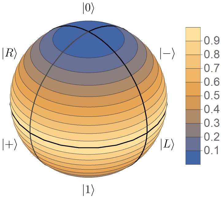
for this general case on the Bloch sphere in Fig. 4.
Next, we consider time evolution. We have
| (68) |
Measuring at time bounds the energy probabilities as
| (69) |
If we measure at different times during , we manage to tighten these bounds and obtain
| (70) |
which leads to bounds on energy
| (71) |
The corresponding quality factor is again plotted in Fig. 4.
Appendix E Estimation of the mean energy in experimentally relevant models
Here we show the simulations for energy estimation using measurements in a local number basis and then using optimized -local measurements. This is a continuation of numerical simulations shown in the main text, which contained a part of the results obtained for the Heisenberg model.
We simulate a number of models, including the Heisenberg model Porras and Cirac (2004); Pal and Huse (2010); Luitz et al. (2015), which is a paradigmatic model to study for many-body localization, and then several other experimentally relevant models. These are the Ising model Smith et al. (2016); Jurcevic et al. (2017); Zhang et al. (2017); Bingham et al. (2021), known for its frequent use in quantum simulators and quantum annealers, the XY model Lanyon et al. (2017); Friis et al. (2018); Brydges et al. (2019); Maier et al. (2019), which is a type of non-integrable long-range model, and the PXP model Bernien et al. (2017); Turner et al. (2018); Su et al. (2022), an archetypal model for many-body quantum scars.
The Hamiltonians and the corresponding parameters are given in Table 1. The simulations of energy estimation using local particle number measurements and optimized -local measurements are shown in Tables 2 and 3.
The bulk of the explanation necessary to understand these numerical experiments are also shown in the main text. Below, we give details on the types of Hilbert space considered in our simulations, and we discuss methods that we designed for the optimization over the -local measurements to estimate energy.
Hilbert space considered. In our simulations, we choose to work in a different type of Hilbert space for each model, depending on the conservation laws, and to match the experimental setups, see Table 1: In the Heisenberg and the XY models, the full Hilbert space splits into subspaces, each of them characterized by a definite value of the total spin along the axes, i.e., . We work in the largest subspace, characterized by the value . This conservation is also why the actual value of in the XY model is irrelevant. For the Ising model, the total spin along the axes is not conserved, only the parity of the total spin is conserved. In this case, we work on the parity even subspace, which contains the Néel state. For the PXP model, the situation is more intricate: the presence of the projector operators in the Hamiltonian introduces a non-trivial local constraint Turner et al. (2018). Consequently, the full Hilbert space shatters in many different subspaces, dynamically disconnected and having various dimensions Khemani et al. (2020). Inside each subspace, the dynamics is generically chaotic with the presence of many-body scars Turner et al. (2018); Serbyn et al. (2021); Chandran et al. (2022). However, our goal in using this model was to study the effect of the Hilbert space shattering on the quality of the energy estimation. Therefore, we work in the full Hilbert space.
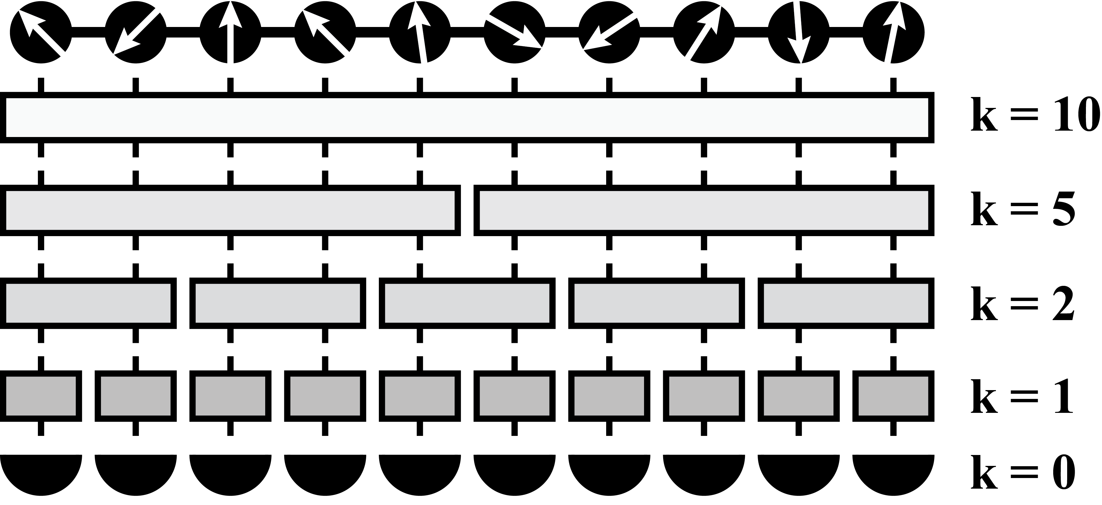
Methods for optimizing local measurements. We introduce three methods of analytical optimization for the -local measurements. The sketch of -local measurements is shown in Fig. 5, which corresponds to Fig 3 (a) in the main text. -local measurement consists of applying a -local unitary operator and then measuring in the computational basis.
| name | characteristics | conservation | Hamiltonian | parameters | |||||||||||||
|
|
|
|
||||||||||||||
|
|
|
|
||||||||||||||
| XY |
|
|
, , | ||||||||||||||
| PXP |
|
|
|||||||||||||||
| Sizes and Hilbert spaces considered in the numerical experiments | |||||||||||||||||
| Small systems | Large systems | ||||||||||||||||
| Heisenberg | 6 sites, 3 particles | 10 sites, 5 particles | |||||||||||||||
| Ising | 6 sites, even parity subspace | 10 sites, even parity subspace | |||||||||||||||
| XY | 6 sites, 3 particles | 10 sites, 5 particles | |||||||||||||||
| PXP | 5 sites, full Hilbert space | 10 sites, full Hilbert space | |||||||||||||||
| initial states: G C H | |||||
| Ham. | small system | large system | |||
| ground state-optimized | observable-optimized | ||||
|
![[Uncaptioned image]](https://cdn.awesomepapers.org/papers/c8e7e6f7-b54d-4868-807a-0734a8b7bfe1/x2.png) |
![[Uncaptioned image]](https://cdn.awesomepapers.org/papers/c8e7e6f7-b54d-4868-807a-0734a8b7bfe1/x3.png) |
|||
|
![[Uncaptioned image]](https://cdn.awesomepapers.org/papers/c8e7e6f7-b54d-4868-807a-0734a8b7bfe1/x5.png) |
![[Uncaptioned image]](https://cdn.awesomepapers.org/papers/c8e7e6f7-b54d-4868-807a-0734a8b7bfe1/x6.png) |
|||
|
![[Uncaptioned image]](https://cdn.awesomepapers.org/papers/c8e7e6f7-b54d-4868-807a-0734a8b7bfe1/x8.png) |
![[Uncaptioned image]](https://cdn.awesomepapers.org/papers/c8e7e6f7-b54d-4868-807a-0734a8b7bfe1/x9.png) |
|||
|
![[Uncaptioned image]](https://cdn.awesomepapers.org/papers/c8e7e6f7-b54d-4868-807a-0734a8b7bfe1/x11.png) |
![[Uncaptioned image]](https://cdn.awesomepapers.org/papers/c8e7e6f7-b54d-4868-807a-0734a8b7bfe1/x12.png) |
|||
|
![[Uncaptioned image]](https://cdn.awesomepapers.org/papers/c8e7e6f7-b54d-4868-807a-0734a8b7bfe1/x14.png) |
![[Uncaptioned image]](https://cdn.awesomepapers.org/papers/c8e7e6f7-b54d-4868-807a-0734a8b7bfe1/x15.png) |
|||
|
![[Uncaptioned image]](https://cdn.awesomepapers.org/papers/c8e7e6f7-b54d-4868-807a-0734a8b7bfe1/x17.png) |
![[Uncaptioned image]](https://cdn.awesomepapers.org/papers/c8e7e6f7-b54d-4868-807a-0734a8b7bfe1/x18.png) |
||
|
![[Uncaptioned image]](https://cdn.awesomepapers.org/papers/c8e7e6f7-b54d-4868-807a-0734a8b7bfe1/x20.png) |
![[Uncaptioned image]](https://cdn.awesomepapers.org/papers/c8e7e6f7-b54d-4868-807a-0734a8b7bfe1/x21.png) |
a. Ground state-optimized measurements. First, we introduce a method that is -local optimization for a specific state, in our case, the ground state. This method is inspired by the Matrix Product State ansatz Orús (2014), and by the correspondence between observational and entanglement entropy Schindler et al. (2020).
The logic of the motivation goes as follows: low observational entropy means that the system state wandered into one of the small subspaces-macrostates given by the measurement Šafránek et al. (2019b); Šafránek and Thingna (2020). This means that we can estimate the maximal and the minimal value of the estimated observable in that subspace, which, in turn, translates into estimating these bounds for the system state itself. In other words, lower observational entropy means better estimates. According to Ref. Schindler et al. (2020), observational entropy minimized over local coarse-grainings leads to entanglement entropy, and the minimum is achieved when the local coarse-grainings are given by the Schmidt basis. This means that the measuring in the Schmidt basis will yield small observational entropy and, in turn, a better estimate of the mean value of observable. Thus, we need to find -local measurements that reflect the Schmidt basis, which are expected to perform well in the estimation.
We do this as follows: Assuming we have a chain of length (for example, ) and some divisor (for example ), we first divide the chain into two parts: one — system — of length (i.e., sites ) and the other — system — of length (i.e., sites ). We define as the ground state (or any other state we want to optimize for). We compute the reduced density matrix
| (72) |
and diagonalize it. The eigenbasis of the reduced density matrix is, by definition, the system -local part of the Schmidt basis. We denote this basis as .
Then we move on to the next sites. We divide the system into (sites ) and (sites ). Again, we compute the reduced density matrix
| (73) |
and find its eigenvectors, which we denote .
We continue dividing the system until the end (in our example, we go up to ). The final, ground state-optimized -local measurement basis is then given by
| (74) |
b. Observable-optimized measurements, type 1. Second, we introduce a method of -local optimization for a specific observable, in our case, the Hamiltonian.
The motivation behind this optimization is that the estimation of the mean value of the observable works better the more the measurement resembles the eigenbasis of the observable. Thus, we create a procedure that generates a measurement that somewhat resembles the estimated observable.
We illustrate this method on the Heisenberg model, assuming , which is given by the Hamiltonian (assuming hard-wall boundary conditions)
| (75) |
For -local measurement, we remove all the terms spanning more than a single site. This leads to a modified Hamiltonian
| (76) |
We call the eigenbasis of this Hamiltonian the -local observable optimized measurement for the Hamiltonian. Incidentally, in this case, this basis is precisely the same as the computational basis.
For -local measurement, we divide the lattice into blocks of two sites and remove all the terms that cross those blocks. This leads to
| (77) |
The eigenbasis of this Hamiltonian is the -local observable optimized measurement for the Hamiltonian.
For -local measurement, we divide the lattice into two blocks of five sites and remove all the terms that cross those blocks. This leads to
| (78) |
The eigenbasis of this Hamiltonian is the -local observable optimized measurement for the Hamiltonian.
In the case of -local measurement, the corresponding Hamiltonian is the original Hamiltonian itself,
| (79) |
Measuring in the basis of this Hamiltonian is the same as measuring the Hamiltonian itself, which yields perfect precision in estimating its mean value.
| initial states: G C H | |
| Ham. | large system |
| observable-optimized (type 2) | |
|
PXP |
 |
c. Observable-optimized measurements, type 2. Alternatively, one can consider a different way of finding observable-optimized measurements, somewhat similar to the ground-state optimization method. For and , divide the system into system (the first two sites ) and system (the last sites ). Then compute the “reduced Hamiltonian”
| (80) |
and diagonalize it, obtaining its eigenbasis . Continue analogously as in the ground-state optimization method to generate the global observable-optimized basis for ,
| (81) |
In our numerical experiments, due to the specific forms of the Hamiltonian, type 1 and type 2 observable-optimized measurements differ only in the PXP model. See Fig. 6.
d. Generating the unitary. Finally, we want to transform the optimized measurement and express it as a combination of a unitary operator applied to the system’s state and, after that measuring in the computational basis. This is illustrated in Fig. 5. Assuming our example and again, we start deriving the formula for with requiring that the probability of an outcome is the same in both situations:
| (82) |
where is the computational basis vector, an optimized basis vector on the first two sites, and we want to match each couple to one . A sufficient condition is
| (83) |
Assuming that is a column vector written in the computational basis and that each site is a qubit (which leads to ), we have
| (84) |
This means that
| (85) |
The global optimized measurement then consists of applying the unitary operation
| (86) |
on the system and then measuring in the computational basis.
References
- D’Alessio et al. (2016) L. D’Alessio, Y. Kafri, A. Polkovnikov, and M. Rigol, Advances in Physics 65, 239 (2016), arXiv:1509.06411 [cond-mat.stat-mech] .
- Deutsch (2018) J. M. Deutsch, Reports on Progress in Physics 81, 082001 (2018), arXiv:1805.01616 [quant-ph] .
- Vojta (2003) M. Vojta, Reports on Progress in Physics 66, 2069 (2003).
- Sun et al. (2014) Z.-Y. Sun, Y.-Y. Wu, J. Xu, H.-L. Huang, B.-F. Zhan, B. Wang, and C.-B. Duan, Phys. Rev. A 89, 022101 (2014).
- Tian et al. (2020) T. Tian, H.-X. Yang, L.-Y. Qiu, H.-Y. Liang, Y.-B. Yang, Y. Xu, and L.-M. Duan, Phys. Rev. Lett. 124, 043001 (2020).
- Yuen and Chan (1983) H. P. Yuen and V. W. S. Chan, Opt. Lett. 8, 177 (1983).
- Tyc and Sanders (2004) T. Tyc and B. C. Sanders, Journal of Physics A: Mathematical and General 37, 7341 (2004).
- Shaked et al. (2018) Y. Shaked, Y. Michael, R. Z. Vered, L. Bello, M. Rosenbluh, and A. Pe’er, Nature Communications 9, 609 (2018).
- Raffaelli et al. (2018) F. Raffaelli, G. Ferranti, D. H. Mahler, P. Sibson, J. E. Kennard, A. Santamato, G. Sinclair, D. Bonneau, M. G. Thompson, and J. C. F. Matthews, Quantum Science and Technology 3, 025003 (2018).
- Noll et al. (1991) D. Noll, D. Nishimura, and A. Macovski, IEEE Transactions on Medical Imaging 10, 154 (1991).
- Voss (2009) P. Voss, Optical homodyne detection and applications in quantum cryptography, Ph.D. thesis, TELECOM ParisTech (2009).
- Davidovich (1996) L. Davidovich, Rev. Mod. Phys. 68, 127 (1996).
- Takeno et al. (2007) Y. Takeno, M. Yukawa, H. Yonezawa, and A. Furusawa, Opt. Express 15, 4321 (2007).
- Lawrie et al. (2019) B. J. Lawrie, P. D. Lett, A. M. Marino, and R. C. Pooser, ACS Photonics 6, 1307 (2019), https://doi.org/10.1021/acsphotonics.9b00250 .
- Heisenberg (1985) W. Heisenberg, in Original Scientific Papers Wissenschaftliche Originalarbeiten (Springer, 1985) pp. 478–504.
- Robertson (1929) H. P. Robertson, Phys. Rev. 34, 163 (1929).
- Busch et al. (2007) P. Busch, T. Heinonen, and P. Lahti, Physics Reports 452, 155 (2007).
- Wightman (1956) A. S. Wightman, Phys. Rev. 101, 860 (1956).
- Srednicki (2007) M. Srednicki, Quantum field theory (Cambridge University Press, 2007).
- Bunge et al. (1993) C. Bunge, J. Barrientos, and A. Bunge, Atomic Data and Nuclear Data Tables 53, 113 (1993).
- Ikot et al. (2019) A. N. Ikot, U. S. Okorie, R. Sever, and G. J. Rampho, European Physical Journal Plus 134, 386 (2019).
- Deutsch (2010) J. M. Deutsch, New Journal of Physics 12, 075021 (2010).
- Swendsen (2015) R. H. Swendsen, arXiv e-prints , arXiv:1508.01323 (2015), arXiv:1508.01323 [cond-mat.stat-mech] .
- Santos et al. (2011) L. F. Santos, A. Polkovnikov, and M. Rigol, Phys. Rev. Lett. 107, 040601 (2011).
- Šafránek et al. (2021) D. Šafránek, A. Aguirre, J. Schindler, and J. M. Deutsch, Foundations of Physics 51, 101 (2021), arXiv:2008.04409 [quant-ph] .
- Hovhannisyan and Correa (2018) K. V. Hovhannisyan and L. A. Correa, Phys. Rev. B 98, 045101 (2018).
- Mukherjee et al. (2019) V. Mukherjee, A. Zwick, A. Ghosh, X. Chen, and G. Kurizki, Communications Physics 2, 1 (2019).
- Cenni et al. (2021) M. F. B. Cenni, L. Lami, A. Acin, and M. Mehboudi, arXiv e-prints , arXiv:2110.02098 (2021), arXiv:2110.02098 [quant-ph] .
- Engel and Nolte (2007) A. Engel and R. Nolte, Europhysics Letters 79, 10003 (2007).
- Alipour et al. (2016) S. Alipour, F. Benatti, F. Bakhshinezhad, M. Afsary, S. Marcantoni, and A. T. Rezakhani, Scientific Reports 6, 35568 (2016), arXiv:1606.08869 [quant-ph] .
- Modak and Rigol (2017) R. Modak and M. Rigol, Phys. Rev. E 95, 062145 (2017).
- Goold et al. (2018) J. Goold, F. Plastina, A. Gambassi, and A. Silva, “The role of quantum work statistics in many-body physics,” in Thermodynamics in the Quantum Regime: Fundamental Aspects and New Directions, edited by F. Binder, L. A. Correa, C. Gogolin, J. Anders, and G. Adesso (Springer International Publishing, Cham, 2018) pp. 317–336.
- De Chiara et al. (2018) G. De Chiara, P. Solinas, F. Cerisola, and A. J. Roncaglia, “Ancilla-assisted measurement of quantum work,” in Thermodynamics in the Quantum Regime: Fundamental Aspects and New Directions, edited by F. Binder, L. A. Correa, C. Gogolin, J. Anders, and G. Adesso (Springer International Publishing, Cham, 2018) pp. 337–362.
- Varizi et al. (2020) A. D. Varizi, A. P. Vieira, C. Cormick, R. C. Drumond, and G. T. Landi, Phys. Rev. Research 2, 033279 (2020).
- Allahverdyan et al. (2004) A. E. Allahverdyan, R. Balian, and T. M. Nieuwenhuizen, Europhysics Letters (EPL) 67, 565 (2004).
- Alicki and Fannes (2013) R. Alicki and M. Fannes, Phys. Rev. E 87, 042123 (2013).
- Šafránek et al. (2022) D. Šafránek, D. Rosa, and F. Binder, arXiv e-prints , arXiv:2209.11076 (2022), arXiv:2209.11076 [quant-ph] .
- Paris (2008) M. G. A. Paris, arXiv e-prints , arXiv:0804.2981 (2008), arXiv:0804.2981 [quant-ph] .
- Correa et al. (2015) L. A. Correa, M. Mehboudi, G. Adesso, and A. Sanpera, Phys. Rev. Lett. 114, 220405 (2015), arXiv:1411.2437 [quant-ph] .
- Mandelstam and Tamm (1991) L. Mandelstam and I. Tamm, “The uncertainty relation between energy and time in non-relativistic quantum mechanics,” in Selected Papers, edited by B. M. Bolotovskii, V. Y. Frenkel, and R. Peierls (Springer Berlin Heidelberg, Berlin, Heidelberg, 1991) pp. 115–123.
- Margolus and Levitin (1998) N. Margolus and L. B. Levitin, Physica D: Nonlinear Phenomena 120, 188 (1998), proceedings of the Fourth Workshop on Physics and Consumption.
- Deffner and Campbell (2017) S. Deffner and S. Campbell, Journal of Physics A Mathematical General 50, 453001 (2017), arXiv:1705.08023 [quant-ph] .
- Villa and De Chiara (2017) L. Villa and G. De Chiara, arXiv e-prints , arXiv:1704.01583 (2017), arXiv:1704.01583 [quant-ph] .
- Jiménez et al. (2021) J. L. Jiménez, S. P. G. Crone, E. Fogh, M. E. Zayed, R. Lortz, E. Pomjakushina, K. Conder, A. M. Läuchli, L. Weber, S. Wessel, A. Honecker, B. Normand, C. Rüegg, P. Corboz, H. M. Rønnow, and F. Mila, Nature (London) 592, 370 (2021).
- Nielsen and Chuang (2002) M. A. Nielsen and I. Chuang, “Quantum computation and quantum information,” (American Association of Physics Teachers, 2002) Chap. 9.3.
- Reich et al. (2013) D. M. Reich, G. Gualdi, and C. P. Koch, Phys. Rev. Lett. 111, 200401 (2013).
- Harper and Flammia (2017) R. Harper and S. T. Flammia, Quantum Science and Technology 2, 015008 (2017), arXiv:1608.02943 [quant-ph] .
- Huang et al. (2019) W. Huang, C. H. Yang, K. W. Chan, T. Tanttu, B. Hensen, R. C. C. Leon, M. A. Fogarty, J. C. C. Hwang, F. E. Hudson, K. M. Itoh, A. Morello, A. Laucht, and A. S. Dzurak, Nature (London) 569, 532 (2019), arXiv:1805.05027 [cond-mat.mes-hall] .
- Combes and Lund (2022) J. Combes and A. P. Lund, arXiv e-prints , arXiv:2207.10210 (2022), arXiv:2207.10210 [quant-ph] .
- Hochbaum (2007) D. S. Hochbaum, Annals of Operations Research 153, 257 (2007).
- Note (1) These are, for example, Nelder-Mead algorithm Luersen and Le Riche (2004), random search Price (1983), differential evolution Storn (1996), machine learning methods Sivanandam and Deepa (2008), simulated Bertsimas and Tsitsiklis (1993) or quantum Das and Chakrabarti (2005) annealing, and modified linear programming methods Powell (1998).
- von Neumann (2010) J. von Neumann, European Physical Journal H 35, 201 (2010).
- Šafránek et al. (2019a) D. Šafránek, J. M. Deutsch, and A. Aguirre, Phys. Rev. A 99, 010101 (2019a), arXiv:1707.09722 [quant-ph] .
- Šafránek et al. (2019b) D. Šafránek, J. M. Deutsch, and A. Aguirre, Phys. Rev. A 99, 012103 (2019b), arXiv:1803.00665 [quant-ph] .
- Strasberg and Winter (2021) P. Strasberg and A. Winter, PRX Quantum 2, 030202 (2021), arXiv:2002.08817 [quant-ph] .
- Buscemi et al. (2022) F. Buscemi, J. Schindler, and D. Šafránek, arXiv:2209.03803 (2022), 10.48550/arXiv.2209.03803.
- Šafránek and Thingna (2020) D. Šafránek and J. Thingna, arXiv e-prints , arXiv:2007.07246 (2020), arXiv:2007.07246 [quant-ph] .
- Usaj et al. (1998) G. Usaj, H. M. Pastawski, and P. R. Levstein, Molecular Physics 95, 1229 (1998), https://doi.org/10.1080/00268979809483253 .
- Sánchez et al. (2016) C. Sánchez, P. Levstein, L. Buljubasich, H. Pastawski, and A. Chattah, Philosophical Transactions of the Royal Society A: Mathematical, Physical and Engineering Sciences 374, 20150155 (2016).
- Pastawski et al. (1995) H. M. Pastawski, P. R. Levstein, and G. Usaj, Phys. Rev. Lett. 75, 4310 (1995).
- Levstein et al. (2004) P. R. Levstein, A. K. Chattah, H. M. Pastawski, J. Raya, and J. Hirschinger, The Journal of Chemical Physics 121, 7313 (2004), https://doi.org/10.1063/1.1792575 .
- Rauer et al. (2018) B. Rauer, S. Erne, T. Schweigler, F. Cataldini, M. Tajik, and J. Schmiedmayer, Science 360, 307 (2018), https://www.science.org/doi/pdf/10.1126/science.aan7938 .
- Abanin et al. (2019) D. A. Abanin, E. Altman, I. Bloch, and M. Serbyn, Rev. Mod. Phys. 91, 021001 (2019).
- Porras and Cirac (2004) D. Porras and J. I. Cirac, Phys. Rev. Lett. 92, 207901 (2004).
- Pal and Huse (2010) A. Pal and D. A. Huse, Phys. Rev. B 82, 174411 (2010).
- Luitz et al. (2015) D. J. Luitz, N. Laflorencie, and F. Alet, Phys. Rev. B 91, 081103 (2015).
- Smith et al. (2016) J. Smith, A. Lee, P. Richerme, B. Neyenhuis, P. W. Hess, P. Hauke, M. Heyl, D. A. Huse, and C. Monroe, Nature Physics 12, 907 (2016), arXiv:1508.07026 [quant-ph] .
- Jurcevic et al. (2017) P. Jurcevic, H. Shen, P. Hauke, C. Maier, T. Brydges, C. Hempel, B. P. Lanyon, M. Heyl, R. Blatt, and C. F. Roos, Phys. Rev. Lett. 119, 080501 (2017).
- Zhang et al. (2017) J. Zhang, G. Pagano, P. W. Hess, A. Kyprianidis, P. Becker, H. Kaplan, A. V. Gorshkov, Z. X. Gong, and C. Monroe, Nature (London) 551, 601 (2017), arXiv:1708.01044 [quant-ph] .
- Bingham et al. (2021) N. S. Bingham, S. Rooke, J. Park, A. Simon, W. Zhu, X. Zhang, J. Batley, J. D. Watts, C. Leighton, K. A. Dahmen, and P. Schiffer, Phys. Rev. Lett. 127, 207203 (2021).
- Lanyon et al. (2017) B. Lanyon, C. Maier, M. Holzäpfel, T. Baumgratz, C. Hempel, P. Jurcevic, I. Dhand, A. Buyskikh, A. Daley, M. Cramer, et al., Nature Physics 13, 1158 (2017).
- Friis et al. (2018) N. Friis, O. Marty, C. Maier, C. Hempel, M. Holzäpfel, P. Jurcevic, M. B. Plenio, M. Huber, C. Roos, R. Blatt, and B. Lanyon, Phys. Rev. X 8, 021012 (2018).
- Brydges et al. (2019) T. Brydges, A. Elben, P. Jurcevic, B. Vermersch, C. Maier, B. P. Lanyon, P. Zoller, R. Blatt, and C. F. Roos, Science 364, 260 (2019).
- Maier et al. (2019) C. Maier, T. Brydges, P. Jurcevic, N. Trautmann, C. Hempel, B. P. Lanyon, P. Hauke, R. Blatt, and C. F. Roos, Phys. Rev. Lett. 122, 050501 (2019).
- Bernien et al. (2017) H. Bernien, S. Schwartz, A. Keesling, H. Levine, A. Omran, H. Pichler, S. Choi, A. S. Zibrov, M. Endres, M. Greiner, V. Vuletić, and M. D. Lukin, Nature (London) 551, 579 (2017), arXiv:1707.04344 [quant-ph] .
- Turner et al. (2018) C. J. Turner, A. A. Michailidis, D. A. Abanin, M. Serbyn, and Z. Papić, Nature Physics 14, 745 (2018).
- Su et al. (2022) G.-X. Su, H. Sun, A. Hudomal, J.-Y. Desaules, Z.-Y. Zhou, B. Yang, J. C. Halimeh, Z.-S. Yuan, Z. Papić, and J.-W. Pan, arXiv e-prints , arXiv:2201.00821 (2022), arXiv:2201.00821 [cond-mat.quant-gas] .
- Bethe (1931) H. Bethe, Zeitschrift für Physik 71, 205 (1931).
- Powell (1994) M. J. Powell, in Advances in optimization and numerical analysis (Springer, 1994) pp. 51–67.
- Powell (1998) M. J. Powell, Acta numerica 7, 287 (1998).
- Huang et al. (2020) H.-Y. Huang, R. Kueng, and J. Preskill, Nature Physics 16, 1050 (2020), arXiv:2002.08953 [quant-ph] .
- Zhao et al. (2021) A. Zhao, N. C. Rubin, and A. Miyake, Phys. Rev. Lett. 127, 110504 (2021).
- Hadfield et al. (2022) C. Hadfield, S. Bravyi, R. Raymond, and A. Mezzacapo, Communications in Mathematical Physics 391, 951 (2022).
- Bu et al. (2022) K. Bu, D. Enshan Koh, R. J. Garcia, and A. Jaffe, arXiv e-prints , arXiv:2202.03272 (2022), arXiv:2202.03272 [quant-ph] .
- Sack et al. (2022) S. H. Sack, R. A. Medina, A. A. Michailidis, R. Kueng, and M. Serbyn, PRX Quantum 3, 020365 (2022).
- Ippoliti (2023) M. Ippoliti, arXiv e-prints , arXiv:2305.10723 (2023), arXiv:2305.10723 [quant-ph] .
- Hu and You (2022) H.-Y. Hu and Y.-Z. You, Phys. Rev. Res. 4, 013054 (2022).
- Hu et al. (2023) H.-Y. Hu, S. Choi, and Y.-Z. You, Phys. Rev. Res. 5, 023027 (2023).
- Gresch and Kliesch (2023) A. Gresch and M. Kliesch, arXiv e-prints , arXiv:2301.03385 (2023), arXiv:2301.03385 [quant-ph] .
- Akhtar et al. (2023) A. A. Akhtar, H.-Y. Hu, and Y.-Z. You, Quantum 7, 1026 (2023).
- Seif et al. (2023) A. Seif, Z.-P. Cian, S. Zhou, S. Chen, and L. Jiang, PRX Quantum 4, 010303 (2023).
- Zhang et al. (2021) T. Zhang, J. Sun, X.-X. Fang, X.-M. Zhang, X. Yuan, and H. Lu, Phys. Rev. Lett. 127, 200501 (2021).
- Struchalin et al. (2021) G. Struchalin, Y. A. Zagorovskii, E. Kovlakov, S. Straupe, and S. Kulik, PRX Quantum 2, 010307 (2021).
- Benedetti et al. (2016) M. Benedetti, J. Realpe-Gómez, R. Biswas, and A. Perdomo-Ortiz, Phys. Rev. A 94, 022308 (2016).
- Pino and García-Ripoll (2020) M. Pino and J. J. García-Ripoll, Phys. Rev. A 101, 032324 (2020).
- Hauke et al. (2020) P. Hauke, H. G. Katzgraber, W. Lechner, H. Nishimori, and W. D. Oliver, Reports on Progress in Physics 83, 054401 (2020), arXiv:1903.06559 [quant-ph] .
- Imoto et al. (2021) T. Imoto, Y. Seki, Y. Matsuzaki, and S. Kawabata, arXiv e-prints , arXiv:2102.05323 (2021), arXiv:2102.05323 [quant-ph] .
- Mohseni et al. (2019) N. Mohseni, M. Narozniak, A. N. Pyrkov, V. Ivannikov, J. P. Dowling, and T. Byrnes, arXiv e-prints , arXiv:1909.09947 (2019), arXiv:1909.09947 [quant-ph] .
- Eisert et al. (2010) J. Eisert, M. Cramer, and M. B. Plenio, Rev. Mod. Phys. 82, 277 (2010).
- Hastings (2007) M. B. Hastings, Journal of Statistical Mechanics: Theory and Experiment 2007, P08024 (2007).
- Terhal (2000) B. M. Terhal, Physics Letters A 271, 319 (2000), arXiv:quant-ph/9911057 [quant-ph] .
- Barbieri et al. (2003) M. Barbieri, F. De Martini, G. Di Nepi, P. Mataloni, G. M. D’Ariano, and C. Macchiavello, Phys. Rev. Lett. 91, 227901 (2003).
- Lewenstein et al. (2000) M. Lewenstein, B. Kraus, J. I. Cirac, and P. Horodecki, Phys. Rev. A 62, 052310 (2000).
- Orús (2014) R. Orús, Annals of Physics 349, 117 (2014).
- Schindler et al. (2020) J. Schindler, D. Šafránek, and A. Aguirre, Phys. Rev. A 102, 052407 (2020).
- Swamy (1973) K. Swamy, IEEE Transactions on Automatic Control 18, 306 (1973).
- Khemani et al. (2020) V. Khemani, M. Hermele, and R. Nandkishore, Phys. Rev. B 101, 174204 (2020).
- Serbyn et al. (2021) M. Serbyn, D. A. Abanin, and Z. Papić, Nature Physics 17, 675 (2021).
- Chandran et al. (2022) A. Chandran, T. Iadecola, V. Khemani, and R. Moessner, “Quantum many-body scars: A quasiparticle perspective,” (2022).
- Luersen and Le Riche (2004) M. A. Luersen and R. Le Riche, Computers & Structures 82, 2251 (2004), computational Structures Technology.
- Price (1983) W. Price, Journal of optimization theory and applications 40, 333 (1983).
- Storn (1996) R. Storn, in Proceedings of north american fuzzy information processing (Ieee, 1996) pp. 519–523.
- Sivanandam and Deepa (2008) S. Sivanandam and S. Deepa, in Introduction to genetic algorithms (Springer, 2008) pp. 165–209.
- Bertsimas and Tsitsiklis (1993) D. Bertsimas and J. Tsitsiklis, Statistical science 8, 10 (1993).
- Das and Chakrabarti (2005) A. Das and B. K. Chakrabarti, Quantum annealing and related optimization methods, Vol. 679 (Springer Science & Business Media, 2005).