Measuring Adversarial Robustness using a Voronoi-Epsilon Adversary

Hyeongji Kim Department of Informatics, University of Bergen, Norway Institute of Marine Research, Bergen, Norway Pekka Parviainen Department of Informatics, University of Bergen, Norway Ketil Malde Department of Informatics, University of Bergen, Norway Institute of Marine Research, Bergen, Norway

Abstract

Previous studies on robustness have argued that there is a tradeoff between accuracy and adversarial accuracy. The tradeoff can be inevitable even when we neglect generalization. We argue that the tradeoff is inherent to the commonly used definition of adversarial accuracy, which uses an adversary that can construct adversarial points constrained by $\epsilon$ -balls around data points. As $\epsilon$ gets large, the adversary may use real data points from other classes as adversarial examples. We propose a Voronoi-epsilon adversary which is constrained both by Voronoi cells and by $\epsilon$ -balls. This adversary balances between two notions of perturbation. As a result, adversarial accuracy based on this adversary avoids a tradeoff between accuracy and adversarial accuracy on training data even when $\epsilon$ is large. Finally, we show that a nearest neighbor classifier is the maximally robust classifier against the proposed adversary on the training data.

1 Introduction

By applying a carefully crafted, but imperceptible perturbation to input images, so-called adversarial examples can be constructed that cause classifiers to misclassify the perturbed inputs (Szegedy et al., 2013). Defense methods like adversarial training (Madry et al., 2017) and certified defenses (Wong & Kolter, 2018) against adversarial examples have often resulted in decreased accuracies on clean samples (Tsipras et al., 2018). Previous studies have argued that the tradeoff between accuracy and adversarial accuracy may be inevitable in classifiers (Tsipras et al., 2018; Dohmatob, 2018; Zhang et al., 2019).

1.1 Problem Settings

Problem setting.

Let $\mathcal{X}\subset\mathbb{R}^{\dim}$ be a nonempty input space and $\mathcal{Y}$ be a set of possible classes. Data points $x\in\mathcal{X}$ and corresponding classes $c_{x}\in\mathcal{Y}$ are sampled from a joint distribution $\mathcal{D}$ . The distribution $\mathcal{D}$ should satisfy the condition that $c_{x}$ is unique for all $x$ . The set of the data points is denoted as $X$ . $X$ is a nonempty finite set. A classifier $f$ assigns a class label from $\mathcal{Y}$ for each point $x\in\mathcal{X}$ . $L(x,y)$ is a classification loss of the classifier $f$ provided an input $x\in\mathcal{X}$ and a label $y\in\mathcal{Y}$ .

More notations are summarized in A.1. Abbreviations are summarized in A.2. We focus on situations that we neglect generalization to simplify the analysis.

1.2 Adversarial Accuracy (AA)

Adversarial accuracy is a commonly used measure of adversarial robustness of classifiers (Madry et al., 2017; Tsipras et al., 2018). It is defined by an adversary region $R(x)\subset\mathcal{X}$ , which is an allowed region of the perturbations for a data point $x$ .

Definition 1 (Adversarial accuracy).

Given an adversary that is constrained to an adversary region $R({x})$ , adversarial accuracy $a$ is defined as follows.

a=\mathbb{E}_{(x,c_{x})\sim\mathcal{D}}\left[{\mathds{1}\left(f(x^{*})=c_{x}\right)}\right]\text{ where }x^{*}=\operatorname*{arg\,max}\limits_{x^{\prime}\in R({x})}{L(x^{\prime},c_{x})}

The choice of $R({x})$ will determine the adversarial accuracy that we are measuring. Commonly considered adversary region is $\mathbb{B}(x,\epsilon)$ , which is a $\epsilon$ -ball around a data point $x$ based on a distance metric $d$ (Biggio et al., 2013; Madry et al., 2017; Tsipras et al., 2018; Zhang et al., 2019).

Definition 2 (Standard adversarial accuracy).

When the adversary region is $\mathbb{B}(x,\epsilon)$ , we refer to the adversarial accuracy $a$ as standard adversarial accuracy (SAA) $a_{std}(\epsilon)$ . For SAA, we denote $R({x})$ as $R_{std}({\epsilon;x})$ .

a_{std}(\epsilon)=\mathbb{E}_{(x,c_{x})\sim\mathcal{D}}\left[{\mathds{1}\left(f(x^{*})=c_{x}\right)}\right]\text{ where }x^{*}=\operatorname*{arg\,max}\limits_{x^{\prime}\in R_{std}({\epsilon;x})}{L(x^{\prime},c_{x})}

This adversary region $\mathbb{B}(x,\epsilon)$ is based on an implicit assumption that there might be an adequate single epsilon $\epsilon$ that perturbed samples do not change their classes. However, this assumption has some limitations. We explain that in the next section.

1.3 The Tradeoff Between Accuracy and Standard Adversarial Accuracy

The usage of $\epsilon$ -ball-based adversary can cause the tradeoff between accuracy and adversarial accuracy. When the two clean samples $x_{1}$ and $x_{2}$ with $d(x_{1},x_{2})\leq\epsilon$ have different classes, the increase of standard adversarial accuracy requires misclassification. We illustrate this with a toy example.

1.3.1 Toy Example

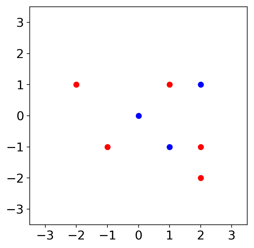
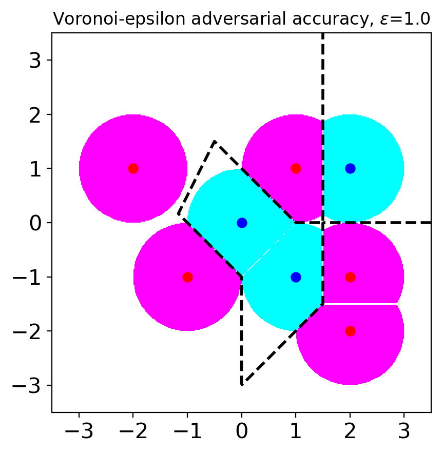
Let us consider an example visualized in Figure 1(a). The input space is $\mathbb{R}^{2}$ . There are only two classes $A$ and $B$ , i.e., $\mathcal{Y}=\left\{A,B\right\}$ . We use the $l_{2}$ norm as a distance metric in this example.

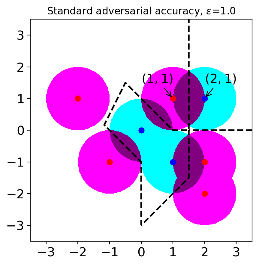
Let us consider a situation when $\epsilon=1.0$ (see Figure 1(c)). In this case, clean samples can also be considered as adversarial examples. For example, the point $(2,1)$ can be considered as an adversarial example originating from the point $(1,1)$ . If we choose a robust model based on SAA, we might choose a model with excessive invariance. For example, we might choose a model that predicts points belong to $\mathbb{B}((1,1),1)$ (including the point $(2,1)$ ) have class A. Or, we can choose a model that predicts points belong to $\mathbb{B}((2,1),1)$ (including the point $(1,1)$ ) have class B. In either case, the accuracy of the chosen model is smaller than $1$ . This situation explains the tradeoff between accuracy and standard adversarial accuracy when large $\epsilon$ is used. It originates from the overlapping adversary regions from the samples with different classes.

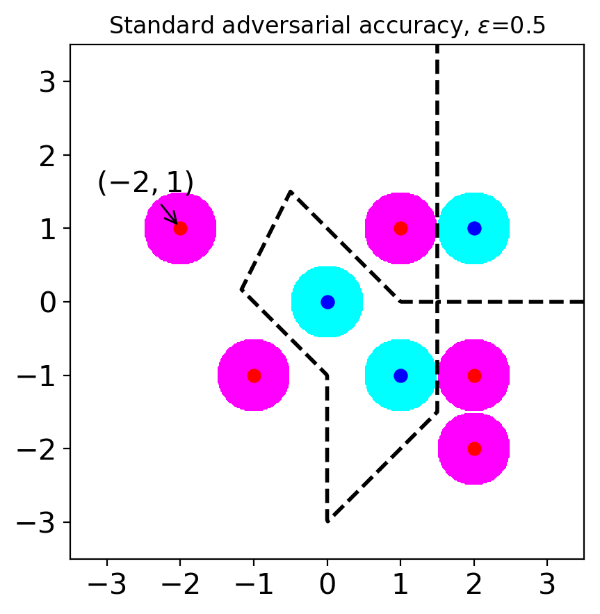
To avoid the tradeoff between accuracy and adversarial accuracy, one can use small $\epsilon$ values. Actually, a previous study has argued that commonly used $\epsilon$ values are small enough to avoid the tradeoff (Yang et al., 2020b). However, when small $\epsilon$ values are used, we can only analyze local robustness, and we need to ignore robustness beyond the chosen $\epsilon$ . For instance, let us consider our example when $\epsilon=0.5$ (see Figure 1(b)). In this case, we ignore robustness on $\mathbb{B}((-2,1),1.0)-\mathbb{B}((-2,1),0.5)$ . Models with local but without global robustness enable attackers to use large $\epsilon$ values to fool the models. Ghiasi et al. (2019) have experimentally shown that even models with certified local robustness can be attacked by attacks with large $\epsilon$ values. Note that their attack applies little semantic perturbations even though the perturbation norms measured by $l_{p}$ norms are large.

These limitations motivate us to find an alternative way to measure robustness. The contributions of this paper are as follows.

•

We propose Voronoi-epsilon adversarial accuracy (VAA) that avoids the tradeoff between accuracy and adversarial accuracy. This allows the adversary regions to scale to cover most of the input space without incurring a tradeoff. To our best knowledge, this is the first work to achieve this without an external classifier. (In Section A.3, we introduce formulas for adversary regions that can be used to estimate VAA.)
•

We explain the connection between SAA and VAA. We define global Voronoi-epsilon robustness as a limit of the Voronoi-epsilon adversarial accuracy. We show that a nearest neighbor (1-NN) classifier maximizes global Voronoi-epsilon robustness.

2 Voronoi-Epsilon Adversarial Accuracy (VAA)

Our approach restricts the allowed region of the perturbations to avoid the tradeoff originating from the definition of standard adversarial accuracy. This is achieved without limiting the magnitude of $\epsilon$ and without using an external model. We want to have the following property to avoid the tradeoff.

\displaystyle\forall x_{i},x_{j}\in X,\,\,x_{i}\neq x_{j}\Longrightarrow R(x_{i})\cap R(x_{j})=\varnothing

(1)

When Property (1) holds for the adversary region, we no longer have the tradeoff as $x_{i}\notin R(x_{j})$ for $x_{i}\neq x_{j}$ . In other words, a clean sample cannot be an adversarial example originating from another clean sample. We propose a new adversary called a Voronoi-epsilon adversary that combines the Voronoi-adversary introduced by Khoury & Hadfield-Menell (2019) with an $\epsilon$ -ball-based adversary. This adversary is constrained to an adversary region $Vor(x)\cap\mathbb{B}(x,\epsilon)$ where $Vor(x)$ is the (open) Voronoi cell around a data point $x\in X$ . $Vor(x)$ consists of every point in $\mathcal{X}$ that is closer than any $x_{clean}\in X-\left\{x\right\}$ . Then, Property (1) holds as $Vor(x_{i})\cap Vor(x_{j})=\varnothing$ for $x_{i}\neq x_{j}$ .

Based on a Voronoi-epsilon adversary, we define Voronoi-epsilon adversarial accuracy (VAA).

Definition 3 (Voronoi-epsilon adversarial accuracy).

When a Voronoi-epsilon adversary is used for the adversary, we refer to the adversarial accuracy as Voronoi-epsilon adversarial accuracy (VAA) $a_{Vor}(\epsilon)$ . For VAA, we denote $R({x})$ as $R_{Vor}({\epsilon;x})$ .

a_{Vor}(\epsilon)=\mathbb{E}_{x\in X}\left[{\mathds{1}\left(f(x^{*})=c_{x}\right)}\right]\text{ where }x^{*}=\operatorname*{arg\,max}\limits_{x^{\prime}\in R_{Vor}({\epsilon;x})}{L(x^{\prime},c_{x})}

Note that VAA is only defined on a fixed set of data points $X$ . As we do not know the distribution $\mathcal{D}$ , in practice, the fact that VAA is not defined on the whole input space does not matter.

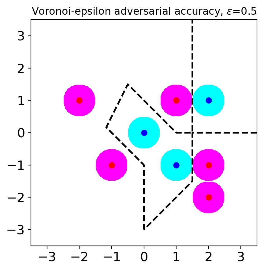
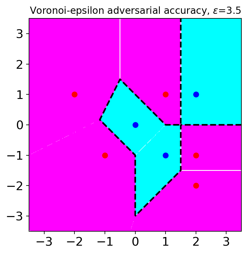
Figure 2 shows the adversary regions for VAA with varying $\epsilon$ values. When $\epsilon=0.5$ , the regions are same with SAA except for the points $(1.5,1),(1.5,-1)$ and $(2,-1.5)$ . Even when $\epsilon$ is large ( $\epsilon>0.5$ ), there is no overlapping adversary region, which was a source of the tradeoff in SAA. Therefore, when we choose a robust model based on VAA, we can get a model that is both accurate and robust. Figure 2(c) shows the single nearest neighbor (1-NN) classifier would maximize VAA. The adversary regions cover most of the points in $\mathbb{R}^{2}$ for large $\epsilon$ .

Observation 1.

Let $d_{min}$ be the nearest distance of the data point pairs, i.e., $d_{min}=\min\limits_{x_{i},x_{j}\in X,x_{i}\neq x_{j}}d(x_{i},x_{j})$ . Then, the following equivalence holds.

\displaystyle a_{Vor}(\epsilon)=a_{std}(\epsilon)\text{ when }\epsilon<\frac{1}{2}d_{min}

(2)

Observation 1 shows that VAA is equivalent to SAA for sufficiently small $\epsilon$ values. This indicates that VAA is an extension of SAA that avoids the tradeoff when $\epsilon$ is large. The proof of the observation is in Section A.5. We point out that equivalent findings were also mentioned in Yang et al. (2020a; b); Khoury & Hadfield-Menell (2019).

As explained in Section 1.3.1, studying the local robustness of classifiers has a limitation. Attackers can attack models with only local robustness by using large $\epsilon$ values. The absence of a tradeoff between accuracy and VAA enables us to increase $\epsilon$ values and to study global robustness. We define a measure for global robustness using VAA.

Definition 4 (Global Voronoi-epsilon robustness).

Global Voronoi-epsilon robustness $a_{global}$ is defined as

a_{global}=\lim\limits_{\epsilon\rightarrow\infty}{a_{Vor}(\epsilon)}.

Global Voronoi-epsilon robustness considers the robustness of classifiers for most points in $\mathcal{X}$ (all points except for Voronoi boundary $VB(X)$ , which is the complement set of the unions of Voronoi cells.). We derive the following theorem from global Voronoi-epsilon robustness.

Theorem 1.

A single nearest neighbor (1-NN) classifier maximizes global Voronoi-epsilon robustness $a_{global}$ on training data. 1-NN classifier is a unique classifier that satisfies this except for Voronoi boundary $VB(X)$ .

Note that Theorem 1 only holds for exactly the same data under the exclusive class condition as mentioned in the problem settings Problem setting. It does not take into account generalization. The proof of the theorem is in A.6.

3 Discussion

In this work, we address the tradeoff between accuracy and adversarial robustness by introducing the Voronoi-epsilon adversary. Another way to address this tradeoff is to use a Bayes optimal classifier (Suggala et al., 2019; Kim & Wang, 2020). Since this is not available in practice, a reference model must be used as an approximation. In that case, the meaning of adversarial robustness is dependent on the choice of the reference model. VAA removes the need for a reference model by using the data point set $X$ and the distance metric $d$ to construct adversary. This is in contrast to Khoury & Hadfield-Menell (2019) who used Voronoi cell-based constraints (without $\epsilon$ -balls) for an adversarial training purpose, but not for measuring adversarial robustness.

By avoiding the tradeoff with VAA, we can extend the study of local robustness to global robustness. Also, Theorem 1 implies that VAA is a measure of agreement with the 1-NN classifier. For sufficiently small $\epsilon$ values, SAA is also a measure of agreement with the 1-NN classifier because SAA is equivalent to VAA as in Observation 1. This implies that many defenses (Goodfellow et al., 2014; Madry et al., 2017; Zhang et al., 2019; Wong & Kolter, 2018; Cohen et al., 2019) with small $\epsilon$ values unknowingly try to make locally the same predictions with a 1-NN classifier.

In our analysis, we do not consider generalization, and robust models are known to often generalize poorly (Raghunathan et al., 2020). The close relationship between adversarially robust models and the 1-NN classifier revealed by Theorem 1 highlights a possible avenue to explore this phenomenon.

Acknowledgments

We thank Dr. Nils Olav Handegard, Dr. Yi Liu, and Jungeum Kim for the helpful feedback. We also thank Dr. Wieland Brendel for the helpful discussions.

References

Biggio et al. (2013) Battista Biggio, Igino Corona, Davide Maiorca, Blaine Nelson, Nedim Šrndić, Pavel Laskov, Giorgio Giacinto, and Fabio Roli. Evasion attacks against machine learning at test time. In Joint European conference on machine learning and knowledge discovery in databases, pp. 387–402. Springer, 2013.
Cohen et al. (2019) Jeremy Cohen, Elan Rosenfeld, and Zico Kolter. Certified adversarial robustness via randomized smoothing. In International Conference on Machine Learning, pp. 1310–1320. PMLR, 2019.
Dohmatob (2018) Elvis Dohmatob. Limitations of adversarial robustness: strong No Free Lunch Theorem. arXiv:1810.04065 [cs, stat], October 2018. URL http://arxiv.org/abs/1810.04065. arXiv: 1810.04065.
Ghiasi et al. (2019) Amin Ghiasi, Ali Shafahi, and Tom Goldstein. Breaking certified defenses: Semantic adversarial examples with spoofed robustness certificates. In International Conference on Learning Representations, 2019.
Goodfellow et al. (2014) Ian J Goodfellow, Jonathon Shlens, and Christian Szegedy. Explaining and harnessing adversarial examples. arXiv preprint arXiv:1412.6572, 2014.
Khoury & Hadfield-Menell (2019) Marc Khoury and Dylan Hadfield-Menell. Adversarial training with Voronoi constraints. arXiv preprint arXiv:1905.01019, 2019.
Kim & Wang (2020) Jungeum Kim and Xiao Wang. Sensible adversarial learning, 2020. URL https://openreview.net/forum?id=rJlf_RVKwr.
Madry et al. (2017) Aleksander Madry, Aleksandar Makelov, Ludwig Schmidt, Dimitris Tsipras, and Adrian Vladu. Towards deep learning models resistant to adversarial attacks. arXiv preprint arXiv:1706.06083, 2017.
Raghunathan et al. (2020) Aditi Raghunathan, Sang Michael Xie, Fanny Yang, John Duchi, and Percy Liang. Understanding and mitigating the tradeoff between robustness and accuracy. arXiv preprint arXiv:2002.10716, 2020.
Suggala et al. (2019) Arun Sai Suggala, Adarsh Prasad, Vaishnavh Nagarajan, and Pradeep Ravikumar. Revisiting adversarial risk. In The 22nd International Conference on Artificial Intelligence and Statistics, pp. 2331–2339. PMLR, 2019.
Szegedy et al. (2013) Christian Szegedy, Wojciech Zaremba, Ilya Sutskever, Joan Bruna, Dumitru Erhan, Ian Goodfellow, and Rob Fergus. Intriguing properties of neural networks. arXiv preprint arXiv:1312.6199, 2013.
Tsipras et al. (2018) Dimitris Tsipras, Shibani Santurkar, Logan Engstrom, Alexander Turner, and Aleksander Madry. Robustness may be at odds with accuracy. arXiv preprint arXiv:1805.12152, 2018.
Wong & Kolter (2018) Eric Wong and Zico Kolter. Provable defenses against adversarial examples via the convex outer adversarial polytope. In International Conference on Machine Learning, pp. 5286–5295. PMLR, 2018.
Yang et al. (2020a) Yao-Yuan Yang, Cyrus Rashtchian, Yizhen Wang, and Kamalika Chaudhuri. Robustness for non-parametric classification: A generic attack and defense. In International Conference on Artificial Intelligence and Statistics, pp. 941–951. PMLR, 2020a.
Yang et al. (2020b) Yao-Yuan Yang, Cyrus Rashtchian, Hongyang Zhang, Russ R Salakhutdinov, and Kamalika Chaudhuri. A closer look at accuracy vs. robustness. Advances in Neural Information Processing Systems, 33, 2020b.
Zhang et al. (2019) Hongyang Zhang, Yaodong Yu, Jiantao Jiao, Eric P Xing, Laurent El Ghaoui, and Michael I Jordan. Theoretically principled trade-off between robustness and accuracy. arXiv preprint arXiv:1901.08573, 2019.

Appendix A Appendix

A.1 List of Notation

$\displaystyle\epsilon$	A perturbation budget.
$\displaystyle\dim$	The dimension of the input space.
$\displaystyle\mathcal{X}$	The nonempty input space. $\mathcal{X}\subset\mathbb{R}^{\dim}$ .
$\displaystyle\mathcal{Y}$	The set of possible classes.
$\displaystyle c_{x}$	A corresponding class of a clean data point $x\in\mathcal{X}$ .
$\displaystyle\mathcal{D}$	The joint distribution. $\mathcal{D}\subset\mathcal{X}\times\mathcal{Y}$ .
$\displaystyle X$	The set of data points. We assume it is a nonempty finite set.
$\displaystyle f$	The classifier that we want to analyze. $f:\mathcal{X}\rightarrow\mathcal{Y}$ .
$\displaystyle L(x,y)$	A classification loss of the classifier $f$ provided an input $x\in\mathcal{X}$ and a label $y\in\mathcal{Y}$ .
$\displaystyle R({x})$	An adversary region which is an allowed region of the perturbations for a data point $x$ . It can be depend on a perturbation budget $\epsilon$ .
$\displaystyle\mathds{1}\left({}\right)$	The indicator function. $\mathds{1}\left(True\right)=1$ and $\mathds{1}\left(False\right)=0$ .
$\displaystyle a$	Adversarial accuracy.
$\displaystyle d$	The distance metric that is used for measuring adversarial robustness. It is not limited to $l_{p}$ norms. It can be a learned metric or more complex distance.
$\displaystyle\mathbb{B}(x,\epsilon)$	An $\epsilon$ -ball around a sample $x$ . Mathematically, $\mathbb{B}(x,\epsilon)=\left\{{x^{\prime}\in\mathcal{X}}\|{d(x,x^{\prime})\leq\epsilon}\right\}$ .
$\displaystyle R_{std}({\epsilon;x})$	The allowed regions of the perturbations for standard adversarial accuracy around a data point $x$ . $R_{std}({\epsilon;x})=\mathbb{B}(x,\epsilon)$ .
$\displaystyle a_{std}(\epsilon)$	Standard adversarial accuracy using a perturbation budget $\epsilon$ . In other words, the adversarial accuracy when the adversary region is $R_{std}({\epsilon;x})=\mathbb{B}(x,\epsilon)$ .
$\displaystyle HS(x,x_{clean})$	The (open) half-space closer to $x\in X$ than $x_{clean}\in X-\left\{x\right\}$ . Mathematically, $HS(x,x_{clean})=\left\{x^{\prime}\in\mathcal{X}\|d(x,x^{\prime})<d(x_{clean},x^{\prime})\right\}$ .
$\displaystyle Vor(x)$	The (open) Voronoi cell of a sample $x\in X$ . Mathematically, $Vor(x)=\left\{x^{\prime}\in\mathcal{X}\|d(x,x^{\prime})<d(x_{clean},x^{\prime}),\forall x_{clean}\in X-\left\{x\right\}\right\}=\bigcap\limits_{x_{clean}\in X-\left\{x\right\}}{HS(x,x_{clean})}$ .
$\displaystyle R_{Vor}({\epsilon;x})$	The allowed regions of the perturbations for Voronoi-epsilon adversarial accuracy around a data point $x$ . $R_{Vor}({\epsilon;x})=Vor(x)\cap\mathbb{B}(x,\epsilon)$ .
$\displaystyle a_{Vor}(\epsilon)$	The Voronoi-epsilon adversarial accuracy using perturbation budget $\epsilon$ . In other words, the adversarial accuracy when the adversary region is $R_{Vor}({\epsilon;x})=Vor(x)\cap\mathbb{B}(x,\epsilon)$ .
$\displaystyle S^{\mathsf{c}}$	The complement set of a set $S$ . For $S\subset\mathcal{X}$ , $S^{\mathsf{c}}=\mathcal{X}-S$ .
$\displaystyle VB(X)$	Voronoi boundary based on $X$ . It is the complement set of the unions of Voronoi cells. $VB(X)=\left(\bigcup\limits_{x\in X}{Vor(x)}\right)^{\mathsf{c}}=\bigcap\limits_{x\in X}{Vor(x)^{\mathsf{c}}}$ .
$\displaystyle a_{global}$	Global Voronoi-epsilon robustness.
$\displaystyle N$	The number of data points.
$\displaystyle R_{Vor;LB}({\epsilon;x})$	The allowed regions of the perturbations for the lower bound of Voronoi-epsilon adversarial accuracy around a data point $x$ . When $\epsilon<\frac{1}{2}d(x,x_{m+2})$ , $R_{Vor;LB}({\epsilon;x})=R_{Vor}({\epsilon;x})$ . When $\epsilon\geq\frac{1}{2}d(x,x_{m+2})$ , $R_{Vor;LB}({\epsilon;x})=\mathbb{B}(x,\epsilon)\cap\left(\bigcap\limits_{i=2}^{m+1}{HS(x,x_{i})}\right)$ .

$\displaystyle R_{Vor;UB}({\epsilon;x})$	The allowed regions of the perturbations for the upper bound of Voronoi-epsilon adversarial accuracy around a sample $x$ . When $\epsilon<\frac{1}{2}d(x,x_{m+2})$ , $R_{Vor;UB}({\epsilon;x})=R_{Vor}({\epsilon;x})$ . When $\epsilon\geq\frac{1}{2}d(x,x_{m+2})$ , $R_{Vor;UB}({\epsilon;x})=\mathbb{B}(x,\frac{1}{2}d(x,x_{m+2})-\tau)\cap\left(\bigcap\limits_{i=2}^{m+1}{HS(x,x_{i})}\right)$ .
$\displaystyle a_{Vor;\,LB}(\epsilon)$	The lower bound of Voronoi-epsilon adversarial accuracy using perturbation budget $\epsilon$ . It is defined as the adversarial accuracy when the adversary region for a data point $x$ is $R_{Vor;LB}({\epsilon;x})$ .
$\displaystyle a_{Vor;\,UB}(\epsilon)$	The upper bound of Voronoi-epsilon adversarial accuracy using perturbation budget $\epsilon$ . It is defined as the adversarial accuracy when the adversary region for a data point $x$ is $R_{Vor;UB}({\epsilon;x})$ .

A.2 List of Abbreviation

AA	Adversarial accuracy.
SAA	Standard adversarial accuracy.
VAA	Voronoi-epsilon adversarial accuracy.
1-NN	Single nearest neighbor.
LB	Lower bound.
UB	Upper bound.

A.3 Adversary Region $R_{Vor}({\epsilon;x})$

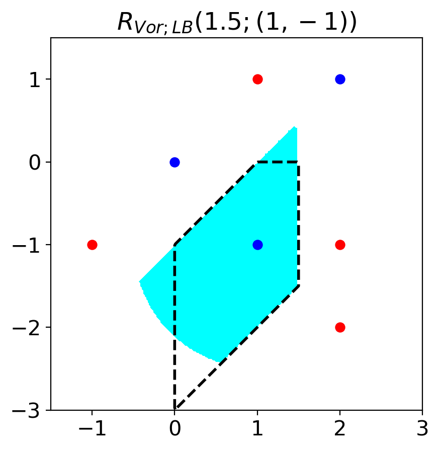
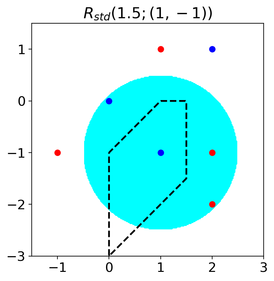
Voronoi-epsilon adversarial accuracy (VAA) uses $R_{Vor}({\epsilon;x})=Vor(x)\cap\mathbb{B}(x,\epsilon)$ . We introduce upper and lower bounds of $R_{Vor}({\epsilon;x})$ using $m+1$ nearest neighbors of a data point $x$ . These bounds enable to calculate approximate upper and lower bounds of VAA.

Lemma 1.

When $N$ is the number of data points, let $x_{2},\cdots,x_{N}\in X-\left\{x\right\}$ be the sorted neighbors of a data point $x\in X$ . Mathematically, $d(x,x_{2})\leq d(x,x_{3})\leq\cdots\leq d(x,x_{N})$ . Then, the following relations hold for a fixed number $m\leq N-2$ . {fleqn}

R_{Vor}({\epsilon;x})=\mathbb{B}(x,\epsilon)\text{ when }\epsilon<\frac{1}{2}d(x,x_{2})

(3)

\begin{split}R_{Vor}({\epsilon;x})=\mathbb{B}(x,\epsilon)\cap\left(\bigcap\limits_{i=2}^{j}{HS(x,x_{i})}\right)\text{ when }\frac{1}{2}d(x,x_{j})\leq\epsilon<\frac{1}{2}d(x,x_{j+1})\\ (j=2,\cdots,m+1)\end{split}

(4)

\begin{split}\mathbb{B}(x,\frac{1}{2}d(x,x_{m+2})-\tau)\cap\left(\bigcap\limits_{i=2}^{m+1}{HS(x,x_{i})}\right)\subset R_{Vor}({\epsilon;x})\subset\mathbb{B}(x,\epsilon)\cap\left(\bigcap\limits_{i=2}^{m+1}{HS(x,x_{i})}\right)\\ \text{ when }\epsilon\geq\frac{1}{2}d(x,x_{m+2})\text{ and }\tau>0\end{split}

(5)

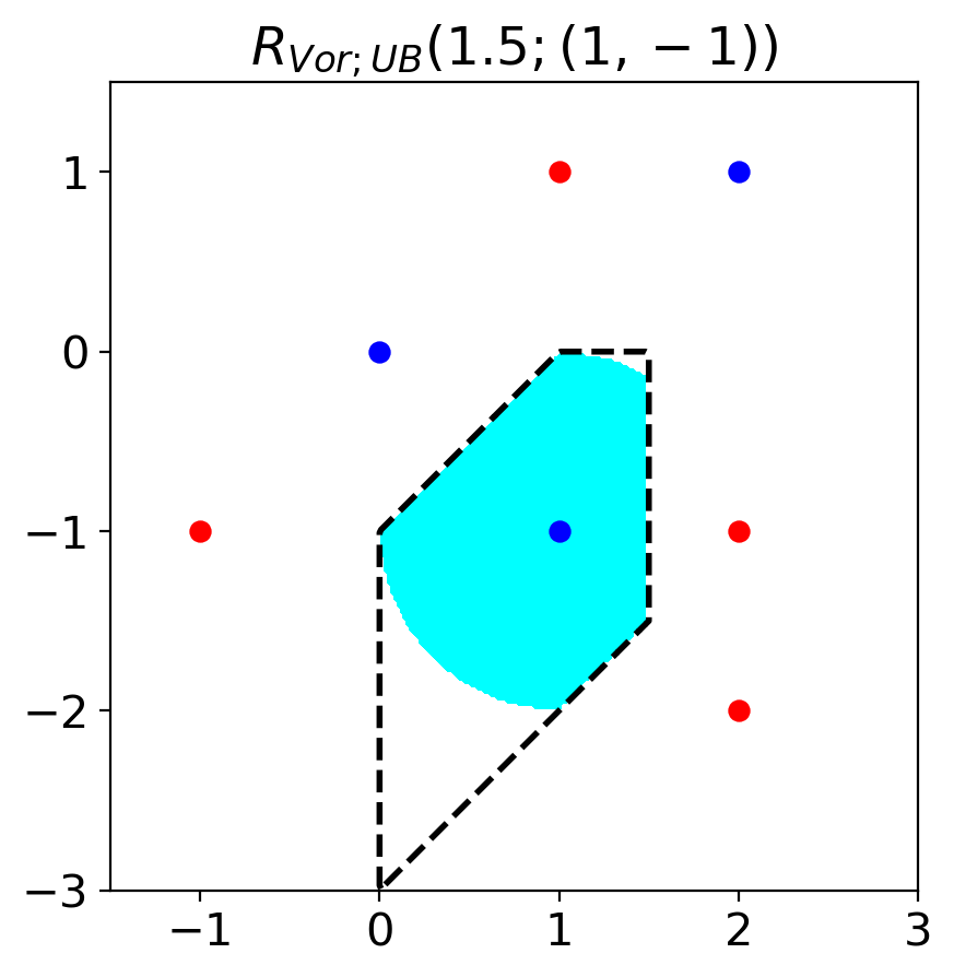
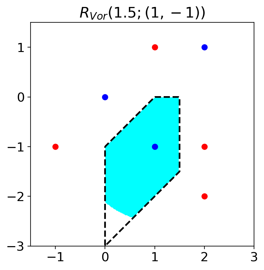
When $\epsilon<\frac{1}{2}d(x,x_{m+2})$ , we can calculate VAA using relations (3) and (4). The relation (5) of Lemma 1 enables to calculate the lower and upper bound of VAA when $\epsilon\geq\frac{1}{2}d(x,x_{m+2})$ . When $\epsilon\geq\frac{1}{2}d(x,x_{m+2})$ , we denote the leftmost set in the relation (5) as $R_{Vor;UB}({\epsilon;x})$ and the rightmost set as $R_{Vor;LB}({\epsilon;x})$ . (When $\epsilon<\frac{1}{2}d(x,x_{m+2})$ , we set $R_{Vor;LB}({\epsilon;x})=R_{Vor;UB}({\epsilon;x})=R_{Vor}({\epsilon;x})$ .) Figure 3 visualizes the relationship $R_{Vor;UB}({\epsilon;x})\subset R_{Vor}({\epsilon;x})\subset R_{Vor;LB}({\epsilon;x})\subset R_{std}({\epsilon;x})$ . The proof of the lemma is in Section A.4.

Proposition 1.

$a_{Vor;\,LB}(\epsilon)$ is defined as the adversarial accuracy when the allowed regions of perturbation is $R_{Vor;LB}({\epsilon;x})$ . $a_{Vor;\,UB}(\epsilon)$ is defined as the adversarial accuracy when the allowed regions of perturbation is $R_{Vor;UB}({\epsilon;x})$ . Then, the following relation holds.

\displaystyle a_{std}(\epsilon)\leq a_{Vor;\,LB}(\epsilon)\leq a_{Vor}(\epsilon)\leq a_{Vor;\,UB}(\epsilon)

(6)

The proof of Proposition 1 is in Section A.5.

A.4 Proof of Lemma 1

Proof.

Relation (3)
First, we consider when $\epsilon<\frac{1}{2}d(x,x_{2})$ .
Let $x^{\prime}\in\mathbb{B}(x,\epsilon)$ . Then, $d(x,x^{\prime})\leq\epsilon$ .
$\frac{1}{2}d(x,x_{2})\leq\frac{1}{2}d(x,x_{clean}),\forall x_{clean}\in X-\left\{x\right\}$ .
Due to the triangle inequality, $\frac{1}{2}d(x,x_{clean})\leq\frac{1}{2}d(x,x^{\prime})+\frac{1}{2}d(x^{\prime},x_{clean})$ .
When we combine the above inequalities, $d(x,x^{\prime})\leq\epsilon<\frac{1}{2}d(x,x_{2})\leq\frac{1}{2}d(x,x_{clean})\leq\frac{1}{2}d(x,x^{\prime})+\frac{1}{2}d(x^{\prime},x_{clean}),\forall x_{clean}\in X-\left\{x\right\}$ .
Then, $\frac{1}{2}d(x,x^{\prime})<\frac{1}{2}d(x^{\prime},x_{clean})=\frac{1}{2}d(x_{clean},x^{\prime}),\forall x_{clean}\in X-\left\{x\right\}$ . Thus, $x^{\prime}\in Vor(x)$ .
Hence, $\mathbb{B}(x,\epsilon)\subset Vor(x)$ and $R_{Vor}({\epsilon;x})=\mathbb{B}(x,\epsilon)\cap Vor(x)=\mathbb{B}(x,\epsilon)$ .
Relation (4)
Now, we consider when $\frac{1}{2}d(x,x_{j})\leq\epsilon<\frac{1}{2}d(x,x_{j+1})\,(j=2,\cdots,m+1)$ .
$R_{Vor}({\epsilon;x})=\mathbb{B}(x,\epsilon)\cap\left(\bigcap\limits_{i=2}^{N-1}{HS(x,x_{i})}\right)\subset\mathbb{B}(x,\epsilon)\cap\left(\bigcap\limits_{i=2}^{j}{HS(x,x_{i})}\right)$ is obvious as $j\leq N-1$ .
We only need to proof $\mathbb{B}(x,\epsilon)\cap\left(\bigcap\limits_{i=2}^{j}{HS(x,x_{i})}\right)\subset R_{Vor}({\epsilon;x})$ .
Let $x^{\prime}\in\mathbb{B}(x,\epsilon)\cap\left(\bigcap\limits_{i=2}^{j}{HS(x,x_{i})}\right)$ . Then, $d(x,x^{\prime})\leq\epsilon,d(x,x^{\prime})<d(x_{2},x^{\prime}),\cdots,d(x,x^{\prime})<d(x_{j},x^{\prime})$ .
$\frac{1}{2}d(x,x_{j+1})\leq\frac{1}{2}d(x,x_{k})$ for $k=j+1,\cdots,N-1$ .
Due to the triangle inequality, $\frac{1}{2}d(x,x_{k})\leq\frac{1}{2}d(x,x^{\prime})+\frac{1}{2}d(x^{\prime},x_{k})$ .
When we combine the above inequalities, $d(x,x^{\prime})\leq\epsilon<\frac{1}{2}d(x,x_{j+1})\leq\frac{1}{2}d(x,x_{k})\leq\frac{1}{2}d(x,x^{\prime})+\frac{1}{2}d(x^{\prime},x_{k})$ for $k=j+1,\cdots,N-1$ .
Then, $\frac{1}{2}d(x,x^{\prime})<\frac{1}{2}d(x^{\prime},x_{k})=\frac{1}{2}d(x_{k},x^{\prime})$ for $k=j+1,\cdots,N-1$ .
We got $d(x,x^{\prime})\leq\epsilon,d(x,x^{\prime})<d(x_{2},x^{\prime}),\cdots,d(x,x^{\prime})<d(x_{N-1},x^{\prime})$ and we proved $\mathbb{B}(x,\epsilon)\cap\left(\bigcap\limits_{i=2}^{j}{HS(x,x_{i})}\right)\subset R_{Vor}({\epsilon;x})$ .
Relation (5)
Finally, we consider when $\epsilon\geq\frac{1}{2}d(x,x_{m+2})$ .
(i) $\mathbb{B}(x,\frac{1}{2}d(x,x_{m+2})-\tau)\cap\left(\bigcap\limits_{i=2}^{m+1}{HS(x,x_{i})}\right)\subset R_{Vor}({\epsilon;x})\text{ for }\tau>0$ :
Let $x^{\prime}\in\mathbb{B}(x,\frac{1}{2}d(x,x_{m+2})-\tau)\cap\left(\bigcap\limits_{i=2}^{m+1}{HS(x,x_{i})}\right)$ . Then, $d(x,x^{\prime})\leq\frac{1}{2}d(x,x_{m+2})-\tau<\frac{1}{2}d(x,x_{m+2})\leq\epsilon,d(x,x^{\prime})<d(x_{2},x^{\prime}),\cdots,d(x,x^{\prime})<d(x_{m+1},x^{\prime})$ .
Through similar process used in the proof of Relation (3) and Relation (4), we have $d(x,x^{\prime})<\frac{1}{2}d(x,x_{m+2})\leq\frac{1}{2}d(x,x_{k})\leq\frac{1}{2}d(x,x^{\prime})+\frac{1}{2}d(x^{\prime},x_{k})$ for $k=m+2,\cdots,N-1$ .
Then, $\frac{1}{2}d(x,x^{\prime})<\frac{1}{2}d(x^{\prime},x_{k})=\frac{1}{2}d(x_{k},x^{\prime})$ for $k=m+2,\cdots,N-1$ .
We got $d(x,x^{\prime})<\epsilon,d(x,x^{\prime})<d(x_{2},x^{\prime}),\cdots,d(x,x^{\prime})<d(x_{N-1},x^{\prime})$ and we proved (i).
(ii) $R_{Vor}({\epsilon;x})\subset\mathbb{B}(x,\epsilon)\cap\left(\bigcap\limits_{i=2}^{m+1}{HS(x,x_{i})}\right)$ :
It is obvious as $R_{Vor}({\epsilon;x})=\mathbb{B}(x,\epsilon)\cap\left(\bigcap\limits_{i=2}^{N-1}{HS(x,x_{i})}\right)$ and $m+1\leq N-1$ . ∎

A.5 Proof of Observation 1 and Proposition 1

Proof.

Observation 1
$d_{min}\leq d(x,x_{i}),$ $\forall x,x_{i}\in X,x\neq x_{i}$ .
When $\epsilon<\frac{1}{2}d_{min}$ , $\epsilon<\frac{1}{2}d_{min}\leq\frac{1}{2}d(x,x_{i}),$ $\forall x,x_{i}\in X,x\neq x_{i}$ . Thus, $R_{Vor}({\epsilon;x})=\mathbb{B}(x,\epsilon),\,\forall x\in X$ due to the relation (3) in Lemma 1.
Then, $a_{Vor}(\epsilon)$ is same with $a_{std}(\epsilon)$ as $R_{Vor}({\epsilon;x})=\mathbb{B}(x,\epsilon)=R_{std}({\epsilon;x})$ $,\forall x\in X$ .
Proposition 1
First, we consider a data point $x\in X$ and let $x_{2},\cdots,x_{N}\in X-\left\{x\right\}$ be the sorted neighbors of $x$ .
Let $x^{*1}=\operatorname*{arg\,max}\limits_{x^{\prime}\in R_{std}({\epsilon;x})}{L(x^{\prime},c_{x})}$ , $x^{*2}=\operatorname*{arg\,max}\limits_{x^{\prime}\in R_{Vor;LB}({\epsilon;x})}{L(x^{\prime},c_{x})}$ , $x^{*3}=\operatorname*{arg\,max}\limits_{x^{\prime}\in R_{Vor}({\epsilon;x})}{L(x^{\prime},c_{x})}$ , and $x^{*4}=\operatorname*{arg\,max}\limits_{x^{\prime}\in R_{Vor;UB}({\epsilon;x})}{L(x^{\prime},c_{x})}$ .
(i) When $\epsilon<\frac{1}{2}d(x,x_{m+2})$ :
$R_{Vor;UB}({\epsilon;x})=R_{Vor}({\epsilon;x})=R_{Vor;LB}({\epsilon;x})$ from the definition.
$R_{Vor;LB}({\epsilon;x})=R_{Vor}({\epsilon;x})\subset\mathbb{B}(x,\epsilon)=R_{std}({\epsilon;x})$ from the relations (3) and (4).
Then, $\mathds{1}\left(f(x^{*1})=c_{x}\right)\leq\mathds{1}\left(f(x^{*2})=c_{x}\right)=\mathds{1}\left(f(x^{*3})=c_{x}\right)=\mathds{1}\left(f(x^{*4})=c_{x}\right)$ as $R_{Vor;UB}({\epsilon;x})=R_{Vor}({\epsilon;x})=R_{Vor;LB}({\epsilon;x})\subset R_{std}({\epsilon;x})$ .
(ii) When $\epsilon\geq\frac{1}{2}d(x,x_{m+2})$ :
$R_{Vor;UB}({\epsilon;x})\subset R_{Vor}({\epsilon;x})\subset R_{Vor;LB}({\epsilon;x})$ from the relation (5).
$R_{Vor;LB}({\epsilon;x})=\mathbb{B}(x,\epsilon)\cap\left(\bigcap\limits_{i=2}^{m+1}{HS(x,x_{i})}\right)\subset\mathbb{B}(x,\epsilon)=R_{std}({\epsilon;x})$ from the definition.
Then, $\mathds{1}\left(f(x^{*1})=c_{x}\right)\leq\mathds{1}\left(f(x^{*2})=c_{x}\right)\leq\mathds{1}\left(f(x^{*3})=c_{x}\right)\leq\mathds{1}\left(f(x^{*4})=c_{x}\right)$ as $R_{Vor;UB}({\epsilon;x})\subset R_{Vor}({\epsilon;x})\subset R_{Vor;LB}({\epsilon;x})\subset R_{std}({\epsilon;x})$ .
From (i) and (ii), $\mathbb{E}_{(x,c_{x})\sim\mathcal{D}}\left[{\mathds{1}\left(f(x^{*1})=c_{x}\right)}\right]\leq\mathbb{E}_{(x,c_{x})\sim\mathcal{D}}\left[{\mathds{1}\left(f(x^{*2})=c_{x}\right)}\right]\leq\mathbb{E}_{(x,c_{x})\sim\mathcal{D}}\left[{\mathds{1}\left(f(x^{*3})=c_{x}\right)}\right]\leq\mathbb{E}_{(x,c_{x})\sim\mathcal{D}}\left[{\mathds{1}\left(f(x^{*4})=c_{x}\right)}\right]$ .
We finished the proof of the relation (6) as $a_{std}(\epsilon)=\mathbb{E}_{(x,c_{x})\sim\mathcal{D}}\left[{\mathds{1}\left(f(x^{*1})=c_{x}\right)}\right]$ , $a_{Vor;\,LB}(\epsilon)=\mathbb{E}_{(x,c_{x})\sim\mathcal{D}}\left[{\mathds{1}\left(f(x^{*2})=c_{x}\right)}\right]$ , $a_{Vor}(\epsilon)=\mathbb{E}_{(x,c_{x})\sim\mathcal{D}}\left[{\mathds{1}\left(f(x^{*3})=c_{x}\right)}\right]$ , and $a_{Vor;\,UB}(\epsilon)=\mathbb{E}_{(x,c_{x})\sim\mathcal{D}}\left[{\mathds{1}\left(f(x^{*4})=c_{x}\right)}\right]$ . ∎

A.6 Proof of Theorem 1

To proof Theorem 1, we introduce the following lemma.

Lemma 2.

By changing $\epsilon$ and $x\in X$ , $x^{\prime}$ that satisfies $x^{\prime}\in R_{Vor}(\epsilon;x)$ can fill up $\mathcal{X}$ except for $VB(X)$ . In other words, $VB(X)^{\mathsf{c}}=\mathcal{X}-VB(X)\subset\bigcup\limits_{\epsilon\geq 0}{\left(\bigcup\limits_{x\in X}{R_{Vor}(\epsilon;x)}\right)}$ .

Proof.

Lemma 2
Let $x^{\prime}\in VB(X)^{\mathsf{c}}$ .
$VB(X)^{\mathsf{c}}=\mathcal{X}-VB(X)=\mathcal{X}-\left(\bigcup\limits_{x\in X}{Vor(x)}\right)^{\mathsf{c}}=\mathcal{X}\cap\left(\bigcup\limits_{x\in X}{Vor(x)}\right)=\bigcup\limits_{x\in X}{Vor(x)}$ .
$\exists x\in X\text{ such that }x^{\prime}\in Vor(x)$ .
Let $\epsilon^{*}=d(x,x^{\prime})$ . Then, $d(x,x^{\prime})\leq\epsilon^{*}$ and $x^{\prime}\in Vor(x)$ .
$x^{\prime}\in\mathbb{B}(x,\epsilon^{*})\cap Vor(x)=R_{Vor}(\epsilon^{*};x)\subset\bigcup\limits_{\epsilon\geq 0}{\left(\bigcup\limits_{x\in X}{R_{Vor}(\epsilon;x)}\right)}$ .
We proved $VB(X)^{\mathsf{c}}\subset\bigcup\limits_{\epsilon\geq 0}{\left(\bigcup\limits_{x\in X}{R_{Vor}(\epsilon;x)}\right)}$ . ∎

Now, we proof Theorem 1.

Proof.

Part 1
First, we prove that a 1-NN classifier maximizes global Voronoi-epsilon robustness. We denote the 1-NN classifier as $f_{1-NN}$ and calculate its global Voronoi-epsilon robustness.
For a data point $x\in X$ , let $x^{\prime}\in R_{Vor}(\epsilon;x)=\mathbb{B}(x,\epsilon)\cap Vor(x)$ .
$x^{\prime}\in Vor(x)\Longleftrightarrow d(x,x^{\prime})<d(x_{clean},x^{\prime}),\forall x\in X-\left\{x\right\}$ .
As $x^{\prime}\in R_{Vor}(\epsilon;x)\subset Vor(x)$ , $x$ is unique nearest data point in $X$ and thus $f_{1-NN}(x^{\prime})=c_{x}$ .
When $x^{*}=\operatorname*{arg\,max}\limits_{x^{\prime}\in R_{Vor}({\epsilon;x})}{L(x^{\prime},c_{x})}$ , $a_{Vor}(\epsilon)=\mathbb{E}_{(x,c_{x})\sim\mathcal{D}}\left[{\mathds{1}\left(f_{1-NN}(x^{*})=c_{x}\right)}\right]=\mathbb{E}_{(x,c_{x})\sim\mathcal{D}}\left[1\right]=1$ .
$a_{global}=\lim\limits_{\epsilon\rightarrow\infty}{a_{Vor}(\epsilon)}=\lim\limits_{\epsilon\rightarrow\infty}{1}=1$ . Thus, $f_{1-NN}$ takes the maximum global Voronoi-epsilon robustness $1$ .

Part 2
Now, we prove that if $f^{*}$ maximizes global Voronoi-epsilon robustness, then $f^{*}$ becomes the 1-NN classifier except for Voronoi boundary $VB(X)$ .
Let $f^{*1}$ be a function that maximizes global Voronoi-epsilon robustness.
From the last part of the part 1, when we calculate global Voronoi-epsilon robustness of $f^{*1}$ , it should satisfy the equation $a_{global}=1$ .
For a data point $x\in X$ and $\epsilon_{1}<\epsilon_{2}$ , $R_{Vor}(\epsilon_{1};x)=\mathbb{B}(x,\epsilon_{1})\cap Vor(x)\subset\mathbb{B}(x,\epsilon_{2})\cap Vor(x)=R_{Vor}(\epsilon_{2};x)$ .
Thus, for a data point $x\in X$ and $\epsilon_{1}<\epsilon_{2}$ , $\mathds{1}\left(f^{*1}(x^{*1})=c_{x}\right)\geq\mathds{1}\left(f^{*1}(x^{*2})=c_{x}\right)$ where $x^{*1}=\operatorname*{arg\,max}\limits_{x^{\prime}\in R_{Vor}({\epsilon_{1};x})}{L(x^{\prime},c_{x})}$ and $x^{*2}=\operatorname*{arg\,max}\limits_{x^{\prime}\in R_{Vor}({\epsilon_{2};x})}{L(x^{\prime},c_{x})}$ .
$a_{Vor}(\epsilon_{1})=\mathbb{E}_{(x,c_{x})\sim\mathcal{D}}\left[{\mathds{1}\left(f^{*1}(x^{*1})=c_{x}\right)}\right]\geq\mathbb{E}_{(x,c_{x})\sim\mathcal{D}}\left[{\mathds{1}\left(f^{*1}(x^{*2})=c_{x}\right)}\right]=a_{Vor}(\epsilon_{2})$ for $\epsilon_{1}<\epsilon_{2}$ . In other words, $a_{Vor}(\epsilon)$ is a decreasing function.
$a_{Vor}(\epsilon)=1,\,\forall\epsilon\geq 0$ ( $\because a_{Vor}(\epsilon^{*})<1$ for a $\epsilon^{*}>0$ , then it is a contradictory to $a_{global}=1$ as $a_{Vor}(\epsilon)$ is a decreasing function.).
$1=a_{Vor}(\epsilon)=\mathbb{E}_{(x,c_{x})\sim\mathcal{D}}\left[{\mathds{1}\left(f^{*1}(x^{*})=c_{x}\right)}\right]$ where $x^{*}=\operatorname*{arg\,max}\limits_{x^{\prime}\in R_{Vor}({\epsilon;x})}{L(x^{\prime},c_{x})}$ .
As the calculation is based on the finite set $X$ , $f^{*1}(x^{*})=c_{x}$ ( $\because{\mathds{1}\left(f^{*1}(x^{*})=c_{x}\right)}=1$ ) where $x^{*}=\operatorname*{arg\,max}\limits_{x^{\prime}\in R_{Vor}({\epsilon;x})}{L(x^{\prime},c_{x})}$ .
As $x^{*}$ are the worst case adversarially perturbed samples, i.e., samples that output mostly different from $c_{x}$ , $f^{*1}(x^{\prime})=c_{x}=f_{1-NN}(x^{\prime})$ where $x^{\prime}\in R_{Vor}({\epsilon;x})$ .
By changing $\epsilon$ and $x\in X$ , $x^{\prime}$ that satisfies $x^{\prime}\in R_{Vor}({\epsilon;x})$ can fill up $\mathcal{X}$ except for $VB(X)$ ( $\because$ Lemma 2). Hence, $f^{*1}$ is equivalent to $f_{1-NN}$ except for Voronoi boundary $VB(X)$ .

∎

Measuring Adversarial Robustness using a Voronoi-Epsilon Adversary

Abstract

1 Introduction

1.1 Problem Settings

Problem setting.

1.2 Adversarial Accuracy (AA)

Definition 1 (Adversarial accuracy).

Definition 2 (Standard adversarial accuracy).

1.3 The Tradeoff Between Accuracy and Standard Adversarial Accuracy

1.3.1 Toy Example

2 Voronoi-Epsilon Adversarial Accuracy (VAA)

Definition 3 (Voronoi-epsilon adversarial accuracy).

Observation 1.

Definition 4 (Global Voronoi-epsilon robustness).

Theorem 1.

3 Discussion

Acknowledgments

References

Appendix A Appendix

A.1 List of Notation

A.2 List of Abbreviation

A.3 Adversary Region RV​o​r​(ϵ;x)R_{Vor}({\epsilon;x})

Lemma 1.

Proposition 1.

A.4 Proof of Lemma 1

Proof.

A.5 Proof of Observation 1 and Proposition 1

Proof.

A.6 Proof of Theorem 1

Lemma 2.

Proof.

Proof.

A.3 Adversary Region $R_{Vor}({\epsilon;x})$