Measurements of $\Sigma$ electromagnetic form factors in the time-like region using the untagged initial-state radiation technique

The inner structure of baryons can be parameterized using electromagnetic form factors (EMFFs). For baryons with spin 1/2, assuming a vector-like current, there are two EMFFs, the magnetic $|G_{\rm M}|$ and the electric $|G_{\rm E}|$ form factors. Experimentally, these can be accessed in the space-like region by electron-baryon elastic scattering and in the time-like region by baryon pair production in electron-positron annihilation Geng:2008mf ; Brodsky:1974vy ; Green:2014xba . Despite the fact that much work has been done on the EM structures of protons in both the space-like and time-like regions Qattan:2004ht ; Puckett:2011xg ; CLEO:2005tiu ; BaBar:2013ves ; CMD-3:2015fvi ; BESIII:2019hdp , experimental information regarding the EMFFs of hyperons remains limited.

The cross section for the process $e^{+}e^{-}\to Y\bar{Y}$ via one-photon exchange, where $Y$ denotes a hyperon with spin 1/2, can be expressed in terms of $|G_{\rm E}|$ and $|G_{\rm M}|$ Cabibbo:1961sz :

where $s$ is the square of the center-of-mass (c.m.) energy, $\alpha=1/137.036$ is the fine-structure constant, $\beta=\sqrt{1-4M_{Y}^{2}/s}$ is the velocity of the final hyperon, $\tau=s/4M_{Y}^{2}$, and $M_{Y}$ is the mass of the hyperon. The Coulomb correction factor $C$ Arbuzov:2011ff00 ; Arbuzov:2011ff , accounting for the electromagnetic interaction of charged pointlike fermion pairs in the final state, is 1.0 for pairs of neutral hyperons and $y/(1-e^{-y})$ with $y=\pi\alpha(1+\beta^{2})/\beta$ for pairs of charged hyperons. The effective form factor (FF) BESIII:2015axk defined by

is proportional to the square root of the hyperon pair production cross section.

Experiments have reported cross section measurements for all members of the spin-parity $J^{P}=(1/2)^{+}$ baryon octet as well as the ground state charmed hyperon $\Lambda_{c}^{+}$ and the $\Omega$ baryon of the 3/2 decuplet Huang:2021xte . Especially close to threshold, intriguing differences are observed. The cross sections of $e^{+}e^{-}\to p\bar{p}$ BaBar:2013ves ; CMD-3:2015fvi ; BESIII:2019hdp , $e^{+}e^{-}\to n\bar{n}$ BESIII:2021np , $e^{+}e^{-}\to\Lambda\bar{\Lambda}$ BaBar:2007fsu ; BESIII:2013vfs ; BESIII:2023ioy , and $e^{+}e^{-}\to\Lambda_{c}^{+}\bar{\Lambda}_{c}^{-}$ BESIII:2017kqg ; BESIII:2023kqg are found to have an abnormal, non-vanishing cross section near threshold. However, a comparably significant effect is not observed for the reactions $e^{+}e^{-}\to\Sigma\bar{\Sigma}$ BESIII:2020uqk ; Belle:2022dvb ; BaBar:2007fsu ; BESIII:2022up , $e^{+}e^{-}\to\Xi\bar{\Xi}$ BESIII:2021yup ; BESIII:2021xup , and $e^{+}e^{-}\to\Omega^{-}\bar{\Omega}^{+}$ BESIII:2022kzc . The unexpected threshold behavior is discussed as final-state interactions Dai:2017fwx , bound states or near threshold meson resonances El-Bennich:2008ytt , or an attractive Coulomb interaction Baldini:2007qg ; BaldiniFerroli:2010ruh .

The cross section of the process $e^{+}e^{-}\to\Sigma^{+}\bar{\Sigma}^{-}$ near its production threshold has been measured by the BESIII experiment BESIII:2020uqk using the scan method. A non-zero threshold cross section was observed with a hint of an enhancement at $\sqrt{s}=$ 2.5 GeV. However, due to limited statistics, an unambiguous conclusion cannot be drawn.

In this paper, a new measurement of the pair production cross sections and the effective form factors of $\Sigma$ from the production threshold up to the invariant mass of $\Sigma^{+}\bar{\Sigma}^{-}$ at 3.04 GeV$/c^{2}$ with the BESIII detector located at the BEPCII collider is presented. The measurement uses the initial-state radiation (ISR) process $e^{+}e^{-}\to\gamma^{\rm ISR}\Sigma^{+}\bar{\Sigma}^{-}$, where $\gamma^{\rm ISR}$ is a hard photon emitted from the initial $e^{+}e^{-}$ pair and thus changes the effective c.m. energy of the collision. The differential cross section for the ISR process is largest when $\gamma^{\rm ISR}$ is emitted almost parallel to the beam axis, where it cannot be detected by BESIII. To benefit from the increased cross section, an untagged ISR measurement is performed. The differential cross section for the $e^{+}e^{-}\to\gamma^{\rm ISR}\Sigma^{+}\bar{\Sigma}^{-}$ process, integrated over the $\Sigma^{+}(\bar{\Sigma}^{-})$ momentum and the ISR photon polar angle, reads Kuraev:1985hb :

where $\sigma_{\Sigma^{+}\bar{\Sigma}^{-}}(q^{2})$ is the cross section for the $e^{+}e^{-}\to\Sigma^{+}\bar{\Sigma}^{-}$ process, $q$ is the momentum transfer of the virtual photon, its square equal to the invariant mass squared of $\Sigma^{+}\bar{\Sigma}^{-}$, $x=\frac{2E_{\gamma}^{*}}{\sqrt{s}}=1-\frac{q^{2}}{s}$, and $E_{\gamma}^{*}$ denotes the energy of the ISR photon in the $e^{+}e^{-}$ c.m. system. The function Druzhinin:2011qd

describes the probability for the emission of an ISR photon with energy fraction $x$, where $k=\frac{2\alpha}{\pi}[{\rm ln}\frac{s}{M_{e}^{2}}-1]$ and $M_{e}$ is the mass of the electron.

The BESIII detector BESIII:2009fln records symmetric $e^{+}e^{-}$ collisions provided by the BEPCII storage ring BEPCII , which operates in the c.m. energy range from 2.0 to 4.95 GeV, with a peak luminosity of $1.0\times 10^{33}\rm{cm^{-2}s^{-1}}$ achieved at $\sqrt{s}=$ 3.773 GeV. BESIII has collected large data samples in this energy region BESIII:2020nme . The cylindrical core of the BESIII detector covers 93% of the full solid angle and consists of a helium-based multilayer drift chamber (MDC), a plastic scintillator time-of-flight system (TOF), and a CsI(Tl) electromagnetic calorimeter (EMC), which are all enclosed in a superconducting solenoidal magnet providing a 1.0 T magnetic field Huang:2022wuo . The solenoid is supported by an octagonal flux-return yoke with resistive plate counter based muon identification modules interleaved with steel. The charged-particle momentum resolution at 1 GeV/$c$ is 0.5%, and resolution of the specific ionization energy loss ($dE/dx$) in the MDC is 6% for electrons from Bhabha scattering. The EMC measures photon energies with a resolution of 2.5% (5%) at 1 GeV in the barrel (end cap) region. The time resolution in the TOF barrel region is 68 ps, while that in the end cap region used to be 110 ps. The end cap TOF system was upgraded in 2015 using multi-gap resistive plate chamber technology, providing a time resolution of 60 ps BESIII:27a ; BESIII:28a ; Cao:2020ibk , which benefits 59.6% of the data used in this analysis.

The data sets used in this analysis are collected at twelve c.m. energies between 3.773 and 4.258 GeV and correspond to a total integrated luminosity of 12.0 fb^-1 BESIII:2023ioy . The individual data sets and the respective luminosities are listed in Table 1. A Geant4-based GEANT4:2002zbu Monte Carlo (MC) simulation package is used to determine the detection efficiency, optimize event selection criteria, and estimate background contributions. For the data processing and analysis, the BESIII Offline Software System Asner:2009zza framework is used. The MC simulated samples of the signal channel ($e^{+}e^{-}\to\gamma^{\rm ISR}\Sigma^{+}\bar{\Sigma}^{-}$) are generated with the ConExc generator Ping:2013jka . The ConExc generator considers ISR processes using the radiator function at next-to-leading order accuracy including the vacuum polarization. The cross section line-shape used for the generation of the signal MC samples is taken from Ref. BESIII:2020uqk . The ISR production of vector charmonium states ($e^{+}e^{-}\to\gamma^{\rm ISR}J/\psi$, $\gamma^{\rm ISR}\psi(3686)$) is generated with BesEvtGen Ping:2008zz using the VECTORISR model VECISR1 ; VECISR2 . The angular distributions of the $\Sigma$ in $J/\psi\to\Sigma^{+}\bar{\Sigma}^{-}$ and $\psi(3686)\to\Sigma^{+}\bar{\Sigma}^{-}$ decays are modeled according to experimental data BESIII:2020fqg . Inclusive MC samples at $\sqrt{s}=3.773$ and $4.178$ GeV are used to investigate possible background contamination. They consist of inclusive hadronic processes ($e^{+}e^{-}\to q\bar{q}$, $q=u,d,s$) modeled with the LUARLW Lund at $\sqrt{s}=3.773$ GeV and KKMC Jadach:1999vf ; KKMC1 at $\sqrt{s}=4.178$ GeV. The dominant background channel, $e^{+}e^{-}\to\pi^{0}\Sigma^{+}\bar{\Sigma}^{-}$, is generated exclusively using the phase space ConExc generator.

To select the candidates for $e^{+}e^{-}\to\gamma^{\rm ISR}\Sigma^{+}\bar{\Sigma}^{-}$, the decays of $\Sigma^{+}(\bar{\Sigma}^{-})\to p\pi^{0}(\bar{p}\pi^{0})$ and $\pi^{0}\to\gamma\gamma$ are reconstructed, while the $\gamma^{\rm ISR}$ is not detected.

The number of charged tracks is required to be two with a net charge of zero. These tracks are reconstructed in the MDC and required to have a polar angle $\theta$ within $|\!\cos\theta|<$ 0.93, where $\theta$ is defined with respect to the z-axis, which is the symmetry axis of the MDC.

Furthermore, the distance of closest approach of each charged track to the interaction point is required within 2 cm in the plane perpendicular to the beam and within 10 cm in the direction along the z-axis. The two selected tracks are identified as one proton and one anti-proton by requiring $\mathcal{P}(p)>\mathcal{P}(h)$, where $\mathcal{P}(h)~{}(h=K,\pi)$ are the probabilities for a track to be assigned to a certain hadron type, based on the $dE/dx$ information measured by the MDC and the time measurement in the TOF.

Photon candidates are reconstructed from isolated showers in the EMC. Each photon candidate is required to have a minimum energy of 25 MeV in the EMC barrel region ($|\!\cos\theta|<0.8$) or 50 MeV in the end cap region ($0.86<|\!\cos\theta|<0.92$). To suppress electronic noise and showers unrelated to the event, the difference between the EMC time and the event start time is required to be within (0, 700) ns. At least four good photon candidates are required for each event. The $\pi^{0}$ candidates are reconstructed from pairs of photons with invariant masses such that $[M_{\gamma\gamma}-M_{\pi^{0}}]\in[-60,\ 40]$ MeV/$c^{2}$, where $M_{\pi^{0}}$ is the known $\pi^{0}$ mass taken from the Particle Data Group (PDG) ParticleDataGroup:2022pth . An asymmetrical $\pi^{0}$ mass window is used because the photon energy deposited in the EMC has a long tail on the low energy side. A one-constraint (1C) kinematic fit is performed on the photon pairs, constraining their invariant masses to the nominal $\pi^{0}$ mass. The $\chi^{2}_{1\rm C}$ of this kinematic fit is required to be less than 25 to remove fake candidates. At least two reconstructed $\pi^{0}$ candidates per event are further required, where two $\pi^{0}$ candidates in an event don’t share the same photons.

The $\Sigma^{+}$ and $\bar{\Sigma}^{-}$ candidates are built from the proton, anti-proton, and neutral pion candidates. From all possible combinations, the neutral pion candidates yielding the smallest value of $\sigma_{m}=\sqrt{(M_{p\pi^{0}}-M_{\Sigma})^{2}+(M_{\bar{p}\pi^{0}}-M_{\Sigma})^{2}}$ are assigned to the baryon decay. Here, $M_{\Sigma}$ is the nominal mass of the $\Sigma$ hyperon ParticleDataGroup:2022pth . According to the fit to the $M_{p\pi^{0}(\bar{p}\pi^{0})}$ spectrum with a double Gaussian function, the signal events are expected to be within a $M_{p\pi^{0}(\bar{p}\pi^{0})}$ mass range of [1.16, 1.21] GeV$/c^{2}$.

To further suppress potential background events, the requirements of the ISR photon polar angle $\theta_{\rm miss}<0.25$ radians or $\theta_{\rm miss}>2.90$ radians, and $U_{\rm miss}\in[-0.14,0.06]$ GeV$/c^{2}$ are imposed. Here, $\theta_{\rm miss}$ in the c.m. frame is the opening angle between the momentum of the recoil against the $\Sigma^{+}\bar{\Sigma}^{-}$ system ($P_{\Sigma^{+}\bar{\Sigma}^{-}}^{\rm rec}$) and the beam direction. $U_{\rm miss}=E_{\Sigma^{+}\bar{\Sigma}^{-}}^{\rm rec}-|P_{\Sigma^{+}\bar{\Sigma}^{-}}^{\rm rec}|$, where $E_{\Sigma^{+}\bar{\Sigma}^{-}}^{\rm rec}$ is the energy of the recoil against the $\Sigma^{+}\bar{\Sigma}^{-}$ system.

Figure 1 shows the distribution of $M_{p\pi^{0}}$ versus $M_{\bar{p}\pi^{0}}$ for all data sets combined. The red box denotes the signal region, which is defined by the mass window discussed above. The black boxes denote the sideband regions used to study and subtract the non-resonant background. For events in the signal region, $M_{\Sigma^{+}\bar{\Sigma}^{-}}$ is plotted in Fig. 2, after improving the mass resolution by applying the correction $M_{\Sigma^{+}\bar{\Sigma}^{-}}^{\rm corr}=M_{\Sigma^{+}\bar{\Sigma}^{-}}^{\rm meas}-M_{p\pi^{0}}-M_{\bar{p}\pi^{0}}+2M_{\Sigma}$, where $M_{\Sigma^{+}\bar{\Sigma}^{-}}^{\rm meas}$, $M_{p\pi^{0}}$, and $M_{\bar{p}\pi^{0}}$ are the measured invariant masses of the four hadrons and the (anti-)proton pion pairs, respectively. Throughout this paper, $M_{\Sigma^{+}\bar{\Sigma}^{-}}$ refers to $M_{\Sigma^{+}\bar{\Sigma}^{-}}^{\rm corr}$.

Potential background sources are investigated by analyzing the inclusive MC samples at $\sqrt{s}=$ 3.773 and 4.178 GeV with the generic event type analysis tool TopoAna Zhou:2020ksj . After applying the above selection criteria, two background contributions are found to be insufficiently suppressed: the non-$\Sigma^{+}\bar{\Sigma}^{-}$ channels and the process $e^{+}e^{-}\to\pi^{0}\Sigma^{+}\bar{\Sigma}^{-}$. The non-$\Sigma^{+}\bar{\Sigma}^{-}$ background contributions are estimated with the sideband method from the $M_{p\pi^{0}(\bar{p}\pi^{0})}$ distributions, since the corresponding distributions based on the inclusive MC samples after excluding the contributions of channels containing $\Sigma^{+}\bar{\Sigma}^{-}$ pairs do not exhibit significant structures. The two-dimensional (2D) sideband regions, shown in Fig. 1, are provided in Table 2. The number of the non-$\Sigma^{+}$$\bar{\Sigma}^{-}$ background events is obtained by $N_{\rm non-\Sigma^{+}\bar{\Sigma}^{-}}^{\rm bkg}=\frac{1}{4}\Sigma^{4}_{i}N_{\textrm{BG}i}^{\rm data}$, where $i$ runs over the four black boxes shown in Fig. 1.

Events of $e^{+}e^{-}\to\pi^{0}\Sigma^{+}\bar{\Sigma}^{-}$ are easily mistaken for signal events if one of the photons of the $\pi^{0}$s is undetected. The background contribution to the selected events is estimated by a data-driven approach using the sideband method. To estimate this contribution, a sample of the $e^{+}e^{-}\to\pi^{0}\Sigma^{+}\bar{\Sigma}^{-}$ events is selected from data using a similar procedure as described for the ISR production of $\Sigma^{+}\bar{\Sigma}^{-}$, but reconstructing an additional $\pi^{0}$ candidate instead of a missing photon. The signal and sideband regions are chosen in the same way as described for the signal process (shown in Fig. 1). The number of events of this sample is calculated by $N_{\pi^{0}\Sigma^{+}\bar{\Sigma}^{-}}^{\rm data}=N_{\pi^{0}\Sigma^{+}\bar{\Sigma}^{-}}^{\rm SigReg}-\frac{1}{4}N_{\pi^{0}\Sigma^{+}\bar{\Sigma}^{-}}^{\rm Side}$, where $N_{\pi^{0}\Sigma^{+}\bar{\Sigma}^{-}}^{\rm SigReg}$ and $N_{\pi^{0}\Sigma^{+}\bar{\Sigma}^{-}}^{\rm Side}$ are the numbers of events from the signal and the sideband regions of the $e^{+}e^{-}\to\pi^{0}\Sigma^{+}\bar{\Sigma}^{-}$ sample, respectively. The contribution from remaining $e^{+}e^{-}\to\pi^{0}\Sigma^{+}\bar{\Sigma}^{-}$ background ($N_{\pi^{0}\Sigma^{+}\bar{\Sigma}^{-}}^{\rm bkg}$) among the signal candidates is determined by:

where $\varepsilon_{\rm bkg}^{\rm MC}$ and $\varepsilon_{\pi^{0}\Sigma^{+}\bar{\Sigma}^{-}}^{\rm MC}$ are the detection efficiencies of selecting the $\Sigma^{+}\bar{\Sigma}^{-}$ and $\pi^{0}\Sigma^{+}\bar{\Sigma}^{-}$ candidates, respectively, from the $e^{+}e^{-}\to\pi^{0}\Sigma^{+}\bar{\Sigma}^{-}$ MC samples.

Figure 3 shows the $M_{\Sigma^{+}\bar{\Sigma}^{-}}$ distribution from threshold up to 3.04 GeV$/c^{2}$ for the events selected from all data sets in Table 1. The red and blue histograms indicate the background contributions due to non-$\Sigma^{+}\bar{\Sigma}^{-}$ channels and $e^{+}e^{-}\to\pi^{0}\Sigma^{+}\bar{\Sigma}^{-}$, respectively.

The cross section for the process $e^{+}e^{-}\to\Sigma^{+}\bar{\Sigma}^{-}$ is calculated from the $M_{\Sigma^{+}\bar{\Sigma}^{-}}$ distribution for each data set by

where $\mathcal{B}(\Sigma)$ = ($51.57\pm 0.30$)% and $\mathcal{B}(\pi^{0})$ = ($99.823\pm 0.034$)% are the branching fractions of $\Sigma^{+}/\bar{\Sigma}^{-}\to p\pi^{0}/\bar{p}\pi^{0}$ and $\pi^{0}\to\gamma\gamma$ ParticleDataGroup:2022pth , respectively. $\mathcal{L}_{\rm int}$ is the integrated luminosity, as listed in Table 1. The effective ISR luminosity $(d\mathcal{L}_{\rm int}/dM_{\Sigma^{+}\bar{\Sigma}^{-}})$ $=W(s,x)\mathcal{L}_{\rm int}$ is calculated by Eq. (4). $\varepsilon$ is the detection efficiency determined using the signal MC samples as a function of $M_{\Sigma^{+}\bar{\Sigma}^{-}}$, and combined as the average value weighted by the corresponding effective ISR luminosity. The $(dN^{\rm sig}/dM_{\Sigma^{+}\bar{\Sigma}^{-}})$ is obtained from the $M_{\Sigma^{+}\bar{\Sigma}^{-}}$ distribution of data after subtracting background. The signal yields are extracted by counting the number of observed events in the signal region as shown in Fig. 3.

The spectrum of $M_{\Sigma^{+}\bar{\Sigma}^{-}}$ is divided into eleven mass intervals between the $\Sigma^{+}\bar{\Sigma}^{-}$ production threshold and 3.04 GeV$/c^{2}$, taking into account the mass resolution, which is smaller than fifth of the bin size. Thus, the spectrum is not unfolded for detector resolution effects. The measured cross sections and the $\Sigma$ effective FFs calculated by Eqs. (1) and (2) are listed in Table 3. The $\overline{\varepsilon}$ and $\mathcal{L}_{\rm eff}$ are the average detection efficiency of all data sets weighted by the effective ISR luminosity and the total effective ISR luminosity, respectively. For the $M_{\Sigma^{+}\bar{\Sigma}^{-}}$ intervals of [2.379, 2.44] and [2.92, 2.98] GeV$/c^{2}$ where fewer than ten signals are found, the upper limits of the signal yield at 90% confidence level are calculated using the profile likelihood method Lundberg:2009iu .

Several sources of systematic uncertainty are considered in the cross section measurement, including the tracking and PID efficiencies of charged tracks, the $\pi^{0}$ efficiency correction, the $\Sigma$ mass window, the $U_{\rm miss}$ and $\theta_{\rm miss}$ requirements, the background estimation, the angular distribution, the luminosity, and the branching fractions of intermediate states. The individual contributions are discussed below.

1. 1.

   Tracking and PID efficiencies: The tracking and PID efficiency differences between data and MC simulation for the proton and anti-proton have been studied in different bins of transverse momentum and polar angle from the control samples of $J/\psi\to p\bar{p}\pi^{+}\pi^{-}$ and $\psi(3686)\to p\bar{p}\pi^{+}\pi^{-}$ BESIII:2021wkr . The differences averaged over the transverse momentum and polar angle of $p$ or $\bar{p}$ of the signal MC samples are taken as the correction factors to calculate the nominal efficiencies. The systematic uncertainty is obtained by summing their relative uncertainties in different bins quadratically and is assigned to be 1.6% for each $M_{\Sigma^{+}\bar{\Sigma}^{-}}$ interval.

2. 2.

   $\pi^{0}$ reconstruction: Based on the control samples of $\psi(3686)\to\pi^{0}\pi^{0}J/\psi,J/\psi\to l^{+}l^{-}$ and $e^{+}e^{-}\to\omega\pi^{0}$, the efficiency differences between data and MC simulation are determined as a function of the momentum, $\Delta\varepsilon_{\pi^{0}}(p)=(0.06-2.41p-\sqrt{0.76p^{2}+1.15+0.39p})\%$ BESIII:2021wkr . The systematic uncertainty is obtained by weighting the relative uncertainties according to the momentum distribution in each mass bin,

   $$~{}~{}~{}~{}~{}~{}\Delta\varepsilon_{\pi^{0}}^{\rm rec}(p)=\frac{n_{1}}{N}\Delta\varepsilon_{\pi^{0}}(p_{1})+\frac{n_{2}}{N}\Delta\varepsilon_{\pi^{0}}(p_{2})+...,~{}~{}~{}$$

   (7)

   where $n_{i}$ is the number of $\pi^{0}$ candidates in the $i$-th bin and $N$ is the total number of $\pi^{0}$ candidates, both in the signal MC sample. The systematic uncertainties of the $\pi^{0}$ reconstruction $\Sigma^{+}\to p\pi^{0}$ and $\bar{\Sigma}^{-}\to\bar{p}\pi^{0}$ are both 1.65%. Therefore, the total systematic uncertainty due to the $\pi^{0}$ reconstruction for $e^{+}e^{-}\to\Sigma^{+}\bar{\Sigma}^{-}$  is 3.3%.

3. 3.

   $\Sigma$ mass window and $U_{\rm miss}$ requirement: The uncertainties due to the $\Sigma$ mass window and the $U_{\rm miss}$ requirement are estimated by studying the $\psi(3686)\to\gamma\chi_{c0},\chi_{c0}\to\Sigma^{+}\bar{\Sigma}^{-}$ decay. The difference in the $\Sigma$ mass window (the $U_{\rm miss}$ requirement) between data and MC simulation which is 1.0(1.4)%, is taken as the systematic uncertainty.

4. 4.

   $\theta_{\rm miss}$ requirement: The uncertainty due to the $\theta_{\rm miss}$ requirement is estimated by studying $e^{+}e^{-}\to\gamma^{\rm ISR}J/\psi,J/\psi\to\Sigma^{+}\bar{\Sigma}^{-}$ decay. The difference in the $\theta_{\rm miss}$ requirement between data and MC simulation which is 2.8%, is taken as the systematic uncertainty.

5. 5.

   Background estimation: To estimate the uncertainties on the number of the non-$\Sigma^{+}$$\bar{\Sigma}^{-}$ background events, the 2D sideband regions are changed from [1.10,1.15] and [1.22,1.27] GeV$/c^{2}$ to [1.095,1.145] and [1.225,1.275] GeV$/c^{2}$. The resulting differences to the nominal result are taken as the systematic uncertainties. The uncertainties of the $e^{+}e^{-}\to\pi^{0}\Sigma^{+}\bar{\Sigma}^{-}$ background events are estimated by also changing the 2D sideband regions in the event selection, and are included in each $M_{\Sigma^{+}\bar{\Sigma}^{-}}$ interval. The total uncertainty of the background estimation is determined by the average of the uncertainty of all $M_{\Sigma^{+}\bar{\Sigma}^{-}}$ intervals. Thus, the total systematic uncertainty on the background estimation for each $\Sigma^{+}$$\bar{\Sigma}^{-}$ mass interval is assigned as 2.5% at $\sqrt{s}=$ 3.773 GeV and 1.1% at the other energy points.

6. 6.

   Angular distribution: In this analysis, the signal MC samples are generated according to an homogeneous and isotropic phase space population, and the angular distribution of the $\Sigma^{+}$$\bar{\Sigma}^{-}$ pair, the spin correlation between $\Sigma^{+}$ and $\bar{\Sigma}^{-}$, and the polarization of the $\Sigma^{+}$($\bar{\Sigma}^{-}$) decay are not taken into account. To estimate the uncertainty due to these factors, the signal MC samples with an angular amplitude including these effects are generated. The parametrization of the angular amplitude is the same as that in Ref. BESIII:2020uqk , and the corresponding parameters are set to be 0.56 and 0.25 for the $M_{\Sigma^{+}\bar{\Sigma}^{-}}$ internals from the threshold to 2.68 GeV$/c^{2}$ and from 2.68 to 3.04 GeV$/c^{2}$, respectively. The relative difference of the detection efficiency to that based on the phase space distribution is assigned as the uncertainty.

7. 7.

   Luminosity: The integrated luminosity is measured by using large-angle Bhabha events with an uncertainty of 0.5% at $\sqrt{s}=$ 3.773 GeV BESIII:2015equ and 1.0% at $\sqrt{s}=$ 4.128-4.258 GeV BESIII:2023ioy ; BESIII:2020eyu ; BESIII:2015qfd . Besides, an additional uncertainty of 0.5% is taken from the radiator function Eq. (4) of Ref. Druzhinin:2011qd . Therefore, the total systematic uncertainty associated with the luminosity for each $\Sigma^{+}$$\bar{\Sigma}^{-}$ mass interval is 0.8% at $\sqrt{s}=$ 3.773 GeV and 1.2% at the other energy points.

8. 8.

   Quoted branching fractions: The branching fractions of $\Sigma^{+}\to p\pi^{0}$, $\bar{\Sigma}^{-}\to\bar{p}\pi^{0}$ and $\pi^{0}\to\gamma\gamma$ are quoted from the PDG ParticleDataGroup:2022pth . The total uncertainty associated with the quoted branching fractions is 1.2%.

In this analysis, the data sets taken at twelve c.m. energy points are used and they are separated into two groups. The first group only includes the one at $\sqrt{s}=$ 3.773 GeV and the second group includes the data sets taken at $\sqrt{s}=$ 4.128-4.258 GeV. The uncertainties of the second group are studied together or obtained from the result at $\sqrt{s}=4.178$ GeV. The systematic uncertainties of the combined groups are listed in Table 4 using the two mass intervals with largest statistics as examples. Uncertainties of the two groups are combined as the average value weighted by the individual detection efficiencies and effective ISR luminosities. The weighted average formula is

with

where $\omega_{i}$, $\sigma_{i}$, and $\varepsilon_{i}$ with $i$ = 1, 2 are the weight factor, systematic uncertainty, and detection efficiency for the $i$-th group, $\rho_{ij}$ is the correlation parameter for the $i$-th and $j$-th group. For the contributions to the systematic uncertainties due to background no correlation is assumed ($\rho_{ij}$ = 0), while full correlation is assumed ($\rho_{ij}$ = 1) for all other contributions.

As shown in Fig. 2, masses from the $\Sigma$ pair threshold up to 4.0 GeV$/c^{2}$ can be studied, including the narrow charmonium vector resonances $J/\psi$ and $\psi(3686)$. Thus, it is possible to study the decays of these resonances into pairs of hyperons and to determine the branching fractions $\mathcal{B}(J/\psi,\psi(3686)\to\Sigma^{+}\bar{\Sigma}^{-})$ by using the data sets taken at $\sqrt{s}=3.773$ and 4.178 GeV with the ISR method. After integrating over the ISR photon polar angle, the cross section for ISR production of a narrow vector meson resonance decaying into the final state $\Sigma^{+}\bar{\Sigma}^{-}$ can be calculated by BESIII:1999res :

where $M_{V}$ and $\Gamma(V\to e^{+}e^{-})$ are the mass and electronic width of the vector meson $V$. Here, $V$ are the $J/\psi$ and $\psi(3686)$ with $\Gamma(J/\psi\to e^{+}e^{-})=\Gamma(J/\psi)\cdot\mathcal{B}(J/\psi\to e^{+}e^{-})=(5.529\pm 0.106)$ keV and $\Gamma(\psi(3686)\to e^{+}e^{-})=\Gamma(\psi(3686))\cdot\mathcal{B}(\psi(3686)\to e^{+}e^{-})=(2.331\pm 0.063)$ keV ParticleDataGroup:2022pth , respectively. $\mathcal{B}(V\to\Sigma^{+}\bar{\Sigma}^{-})$ is the branching fraction of $V\to\Sigma^{+}\bar{\Sigma}^{-}$. $W(s,x_{0})$ is calculated using Eq. (4) with $x_{0}=1-M_{V}^{2}/s$. If the cross section is measured, the branching fraction can be calculated by Eq. (9). The cross section can also be written as:

where $N_{V}^{\rm sig}$ is the number of $V$ events. The $\varepsilon_{V}$ is the detection efficiency of $e^{+}e^{-}\to\gamma^{\rm ISR}V\to\gamma^{\rm ISR}\Sigma^{+}\bar{\Sigma}^{-}$ determined from the signal MC samples. The MC samples are generated with $\Sigma$ angular distributions described as $1+\eta\cos^{2}\theta_{\Sigma}$ with $\eta=-0.508$ for $J/\psi$ and $\eta=0.682$ for $\psi(3686)$ BESIII:2020fqg . The remaining parameters in Eq. (10) are consistent with those defined above. 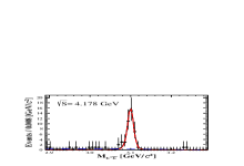To extract $N_{V}^{\rm sig}$, using $\mathcal{B}(V\to\Sigma^{+}\bar{\Sigma}^{-})$ as a shared parameter, a simultaneous fit to the $M_{\Sigma^{+}\bar{\Sigma}^{-}}$ distributions at $\sqrt{s}=3.773$ and 4.178 GeV is performed. The MC simulated shape is used to describe the resonance and a linear function for the background and the continuum contribution. The fit results are shown in Figs. 4(a) and 4(b) for $J/\psi$ and Figs. 4(c) and 4(d) for $\psi(3686)$.

The systematic uncertainties in the measurements of $\mathcal{B}(J/\psi,\psi(3686)\to\Sigma^{+}\bar{\Sigma}^{-})$ include tracking and PID efficiencies of charged tracks, $\pi^{0}$ reconstruction, the $U_{\rm miss}$ requirement, the $\theta_{\rm miss}$ requirement, the $\Sigma$ mass window, the luminosity, and the branching fractions of intermediate states. They are assigned in the same way as for the cross section measurement. In addition, the uncertainty due to the MC model is considered by changing the generator model for the decays of $J/\psi$ or $\psi(3686)$ from HELAMP to AngSam Ping:2008zz . The uncertainty of the fit region is determined by changing the fit region from [2.89, 3.29] GeV/$c^{2}$ to a wider [2.79, 3.30] GeV/$c^{2}$ and a narrower interval [2.94, 3.24] GeV/$c^{2}$. The uncertainty of the signal model is estimated by additionally convolving the signal shape with a Gaussian distribution to account for the possible differences between data and MC simulation. The uncertainty of the background model in the fit is estimated by changing the model from a linear function to a constant, which is found to be negligible. The systematic uncertainties of the measurements of the branching fractions of $J/\psi\to\Sigma^{+}\bar{\Sigma}^{-}$ and $\psi(3686)\to\Sigma^{+}\bar{\Sigma}^{-}$ are listed in Table 5.

The final results for $\mathcal{B}(J/\psi,\psi(3686)\to\Sigma^{+}\bar{\Sigma}^{-})$ with Eqs. (9) and (10) are listed in Table 6. They are consistent with the previous results by BESIII with the data sets taken at the $J/\psi$ or $\psi(3686)$ resonance peak BESIII:2021wkr , showing the reliability of the method of determining the $\Sigma$ EMFFs.

The cross sections measured in Section IV are consistent with the previous results from BESIII BESIII:2020uqk and Belle Belle:2022dvb , as depicted in Fig. 5. A search for a threshold effect is made by performing a least chi-square fit to the cross section in this measurement from the production threshold up to 3.04 GeV$/c^{2}$ and the BESIII scan results BESIII:2020uqk with different functions. The systematic uncertainty is included in the fit with the correlated and uncorrelated parts considered separately.

The perturbative QCD-motivated (pQCD) Pacetti:2014jai energy power function is assumed to model the line-shape of $e^{+}e^{-}\to\Sigma^{+}\bar{\Sigma}^{-}$ production, and the formula is expressed as: