Measurement error models: from nonparametric methods to deep neural networks
Abstract
The success of deep learning has inspired recent interests in applying neural networks in statistical inference. In this paper, we investigate the use of deep neural networks for nonparametric regression with measurement errors. We propose an efficient neural network design for estimating measurement error models, in which we use a fully connected feed-forward neural network (FNN) to approximate the regression function , a normalizing flow to approximate the prior distribution of , and an inference network to approximate the posterior distribution of . Our method utilizes recent advances in variational inference for deep neural networks, such as the importance weight autoencoder, doubly reparametrized gradient estimator, and non-linear independent components estimation. We conduct an extensive numerical study to compare the neural network approach with classical nonparametric methods and observe that the neural network approach is more flexible in accommodating different classes of regression functions and performs superior or comparable to the best available method in nearly all settings.
1 Introduction
The study of nonparametric regression with measurement error is a classical problem in statistics and has received a lot of attentions (Carroll et al.,, 2006). In a typical setting, the response satisfies that , where are the covariates and is an unknown regression function. The covariates are observed with additive errors, i.e., we observe instead of , where is a mean-zero random vector whose distribution is known. Given , the problem of interest is to estimate the nonparametric function .
Most existing methods for fitting measurement error models (MEMs) heavily use classical techniques in nonparametric statistics, such as kernel estimators, splines, and local polynomials. The deconvolution method (Fan and Truong,, 1993) combines the kernel estimator in nonparametric regression with the deconvolution technique in density estimation. Another class of methods approximate the regression function by splines and estimate the spline coefficients using estimating equations (Jiang et al.,, 2018). The simulation extrapolation method (Carroll et al.,, 1999) starts from a standard nonparametric regression method (e.g., splines or local polynomials) and utilizes simulations to estimate and correct its bias when the covariates have errors. While these methods enjoy nice theoretical properties, they still face some major challenges in applications. The first issue is that each method is limited to a particular function class, such as nonparametric functions that are sufficiently smooth or functions that can be well approximated by splines. It is unclear how well they perform when the regression function is generated by a Gaussian process with a non-smooth kernel or when is a complicated function arising from scientific problems. Ideally, we hope to have a method that works for various function classes. Second, these methods require selecting critical tuning parameters, such as the bandwidth in a kernel estimator or the knots for splines. These tuning parameters can significantly affect the performance, but how to select them in a data-driven fashion is a hard problem. Especially, since the common bandwidth selection techniques were mainly designed for nonparametric regression without measurement errors, they may perform unsatisfactorily when the covariates have errors. The third challenge is generalization to multiple covariates (i.e., ). Most existing methods were only studied and evaluated for the case of . Although some of them have extensions to , the practical implementation can be inconvenient. For example, constructing a multivariate kernel estimator requires selecting the optimal bandwidth matrix, which is difficult in practice.
At the same time, the rapid growth of research on deep neural networks opens a new direction for addressing some difficult problems in classical statistics. Attempts have been made for density estimation (Liang,, 2018; Singh et al.,, 2018) and nonparametric regression (Schmidt-Hieber,, 2017; Bauer and Kohler,, 2019). In this paper, we aim to integrate deep neural networks into the estimation of measurement error models. Some nice features of the neural network make it promising for overcoming the challenges faced by classical nonparametric methods. First, it has been widely observed, empirically and theoretically, that deep neural networks have the ability of representing a variety of function classes (Barron,, 1993; Mhaskar,, 1996; Maiorov and Meir,, 2000; Lin et al.,, 2017; Rolnick and Tegmark,, 2018), including many smooth function classes considered in classical nonparametric statistics. Hence, we can potentially use neural networks to develop a universal approach that works for all kinds of function classes. Second, deep neural networks tend to be resistant to overfitting and have great generalization power even when the parameter space has a very high complexity (Golowich et al.,, 2018; Soudry et al.,, 2018). We note that, in classic nonparametric measurement error models, even a moderate significantly increases the complexity of parameter space, and thus may benefit significantly from using neural networks. The tuning for neural networks is also less critical than the selection of smooth parameters (e.g., bandwidth) in nonparametric methods. For the latter, sub-optimal tuning parameters easily lead to overfitting or underfitting. For the former, the major tuning parameters are the architecture of the neural network. We shall use fully connected feed-forward neural networks (FNNs), which boils down to selecting the number of layers and the number of nodes for each layer. The resistance-to-overfitting by neural networks encourages us to set those numbers large without fine tuning.
In this article, we introduce our method of Neural Network for Measurement Error models (NNME), which uses a fully connected FNN to approximate the regression function , a normalizing flow (Tabak and Turner,, 2013) to approximate the prior distribution of , and an inference network (Kingma and Welling,, 2014; Rezende et al.,, 2014) to approximate the posterior distribution of . The training algorithm utilizes some recent advancements in variational inference methods for neural networks, particularly, the importance weighted autoencoder (Burda et al.,, 2016) and the doubly reparametrized gradient estimator (Tucker et al.,, 2018). In fact, viewing the MEM as a latent variable model, our problem has a similar setting as the variational autoencoder (VAE). However, a direct application of VAE yields unsatisfactory performance. There is a nascent literature on improvements and alternatives of VAE (Burda et al.,, 2016; Roeder et al.,, 2017; Le et al.,, 2018; Rainforth et al.,, 2018; Tucker et al.,, 2018), which is unfortunately not familiar to the statistics community. The description of our method also serves as introducing and elaborating these ideas to the statistics community.
We conducted an extensive numerical study to compare NNME with classical nonparametric methods for estimating MEMs. Although the neural network approach is promising, there is no guarantee that it will indeed outperform classical methods. A theoretical comparison is extremely difficult, as the theoretical understanding of deep learning is known to be challenging (Zhang et al.,, 2017). We thus focus on numerical comparison and hope to get a practical guideline of when the neural network method excels and to gain useful insight for future theoretical study. We investigate different function classes for , including smooth functions suitable for classical nonparametric methods, functions generated from Gaussian processes (such functions can be non-smooth), and functions generated by some other unknown neural networks. We discover that the neural network approach has a great flexibility in accommodating different function classes. It has reasonably good performance (sometimes, the best) in all the settings, while each competitor only works well for some specific function classes. In addition, the neural network approach is convenient to apply to the case of multiple covariates, but many classical nonparametric methods are difficult to implement for .
2 The Neural Network for Nonparametric Regression with Measurement Errors
Let be the response, and let be the vector of error-prone covariates. We assume
| (1) | ||||
| (2) |
where are mutually independent, is the (prior) distribution of error-free covariates, and is the distribution of measurement errors satisfying that . Given that are independent and identically distributed (IID) realizations of , the goal is to estimate the regression function . We follow the convention to assume that the analytical form of the measurement error distribution is precisely known (in practice, this distribution is often estimated from other data source or determined by the prior knowledge). The distribution and the variance of observation noise, , are unknown. Note that the assumption that follows a normal distribution is only for convenience. It can be replaced by other parametric distributions, with minor modifications of our method.

2.1 The neural network structure
We use a fully connected feed-forward neural network (FNN) to model the regression function . With denoting parameters of this FNN, we can write . Next, we use a normalizing flow (Tabak and Turner,, 2013) to represent the prior distribution . A normalizing flow is a sequence of transformations , where each is an invertible mapping from to . Let be a random vector whose density has a simple analytic form (e.g., ). We model the density of by assuming , where . Let denote the Jacobian of the mapping . The change of variables formula implies that
By parametrizing each via neural network layers, this idea has been applied to density estimation (Papamakarios et al.,, 2017) and variational inference (Rezende and Mohamed,, 2015). We adopt the specific flow proposed by Dinh et al., (2015), called non-linear independent components estimation (NICE). NICE parametrizes each invertible transformation as follows: and , where is a partition of and is a neural network with input units and output units. Such a mapping has a trivial inverse: and . Furthermore, its Jacobian always has a unit determinant, regardless of the choice of . It thus follows that
| (3) |
Combining (3) with the MEM in (1), we can write down the joint density of :
| (4) |
Here, is the density of measurement errors, which is known; is a simple analytical density, which is typically chosen as the -dimensional standard Gaussian; and is the normal density of noise in . For a moment, we assume is known and write this joint density as . Later, in our main algorithm, will be estimated jointly with other parameters.
Now that the MEM is parametrized by , where contains parameters of interest and contains nuisance parameters, we estimate by maximizing the marginal log-likelihood of the observed variables:
| (5) |
This objective function involves an integral over and cannot be evaluated analytically.
The variational inference is a common tool for parameter estimation and inference in such latent variable models (Jordan et al.,, 1999). The variational auto-encoder (VAE) (Kingma and Welling,, 2014; Rezende et al.,, 2014) is a variational inference approach via neural networks. Standard variational inference approaches approximate the intractable posterior distribution by a parametric family whose densities have simple analytical forms, whereas VAE achieves the same goal by an inference network (also called a recognition model), where the posterior distribution is approximated by a neural network transformation of multivariate normal densities. It has been widely recognized that VAE is capable of approximating complex posterior distributions. Burda et al., (2016) proposed an improvement of VAE by incorporating the idea of importance sampling, namely the importance weighted autoencoder (IWAE). We adapt IWAE to maximize the marginal log-likelihood in (5).
Let be IID samples drawn from a proposal distribution . According to Jensen’s inequality, the marginal log-likelihood has a lower bound:
This lower bound is called an evidence lower bound (ELBO). It is tighter if is closer to the true posterior distribution of and/or is larger.
The idea of VAE is to use a neural network to model the proposal distribution and optimize it jointly with other parameters. However, VAE only corresponds to . One can use the idea of importance sampling (e.g., see Liu, (2008)) with an appropriate sample size to tighten the lower bound. IWAE of Burda et al., (2016) combines these two ideas. We adopt IWAE and model as a multivariate normal distribution , where the vector and the diagonal matrix are both determined by another FNN whose parameters are denoted by . This is equivalent to drawing samples from
| (6) |
Let denote the density of and let be the mapping in (6). We consider the following objective:
| (7) |
The estimator is
| (8) |
The neural network structure that implements this estimator is shown in Figure 1. The FNN parametrized by that generates samples from the proposal distribution is called “encoder.” The FNN parametrized by that approximates the regression function and the normalizing flow parametrized by that approximates the prior distribution of are both called “decoders.” The “encoder” takes data as input, and outputs parameters for the proposal distribution. The “decoders” take as input the random samples generated from the proposal distribution, and outputs the estimated regression function and density at those random samples of .
2.2 The gradient ascent algorithm
We use a gradient ascent algorithm to solve (8). Given initial values , the update at iteration is
| (9) |
where is the step size at iteration , often called the learning rate. We use the adaptive learning rate suggested by Kingma and Ba, (2014), which is , for some default parameters .
It remains to compute the gradient. Write for short , . By direct calculations, we have
| (10) |
The Monte Carlo method approximates the gradients by replacing the expectation in (10) by realized values at a random sample of . At each iteration, we draw IID from and estimate the gradient (10) by
| (11) |
This plain gradient estimator works for approximating and , but not , where we recall that contains parameters in the encoder. The issue of happens when . By theory of IWAE, the objective in (7), as a lower bound of the true marginal log-likelihood, converges to the true marginal log-likelihood as (Burda et al.,, 2016). Therefore, a larger (i.e., more “importance samples”) should be favored. Unfortunately, if (7) is solved by a plain gradient ascent algorithm, the performance is often worse with an increased . The reason is that is too “noisy.” The true gradient vanishes as ; therefore, it is the bias , not the true gradient , that contains the signal. Since the bias diminishes faster than the standard deviation, as increases, the signal-to-noise ratio in the gradient actually decreases. This is, however, not a problem for the gradient with respect to , as the true gradient does not vanish as . See Rainforth et al., (2018) for a rigorous theoretical justification.
Tucker et al., (2018) proposed a method to resolve the above issue. They derived an alternative expression of the gradient with respect to :
| (12) | ||||
| (13) |
where is the same as in (10). We note that (12) cannot be derived from (10) via a simple chain rule. In fact, a direct use of the chain rule should yield a term related to , but there is no such term in (12). This alternative gradient formula motivates another Monte Carlo estimator for :
| (14) |
which is called the doubly reparametrized gradient estimator. Compared with the plain gradient estimator (11), the variance of this estimator converges to zero at a faster rate, so that the signal-to-noise ratio still increases with (see Tucker et al., (2018) for a detailed explanation). The difference between (11) and (14) is analogous to the difference between the score function gradient estimator (or reinforce gradient estimator) and the reparametrization gradient estimator in Monte Carlo variational inference (Kingma and Welling,, 2014; Titsias and Lázaro-Gredilla,, 2014; Rezende et al.,, 2014). It is well-known that the reparametrization gradient estimator has a smaller variance.
2.3 Our method: NNME
Our main algorithm, called Neural Network for Measurement Error (NNME), is summarized in Algorithm 1.
Data: Training data and prespecified values for evaluating .
Input: The density of measurement error,
the neural network structure, parameters , maximum number of epochs , and number of importance samples .
-
1.
Pre-processing: Standardize and each covariate of .
-
2.
Initialization: For each of the two networks representing and , pre-train it using as if there is no measurement error. In pre-training, the loss function is the mean squared error (MSE) plus an L2 penalization term, or . Initialize from pre-training; initialize randomly; and initialize by the MSE from pre-training.
- 3.
Output: The estimated values .
We now provide a more detailed explanation of NNME. Note that the calculations in Sections 2.1-2.2 are for . For a general , write and . At each epoch, we draw samples IID from and obtain . Similar to (11) and (14), we have
| (15) | ||||
where and the expressions of and are given by (4) and (6), respectively. The gradient computation involves calculation of , , and , which are computed via the back propagation algorithm (McClelland et al.,, 1986; Hecht-Nielsen,, 1992). We also use the -regularization trick to reduce numerical instability. We add a penalty to the objective function. It is similar in spirit to the ridge regression and helps stabilize the numerical performance. This penalty changes nothing of the gradient ascent algorithm except for an additional term to each of the gradients ; see Step 3 of Algorithm 1. The noise variance , which is assumed known in derivations of Sections 2.1-2.2, can be estimated along with training the neural network. At each epoch, we estimate by a weighed sum of residuals:
| (16) |
No additional computing effort is needed, since are already obtained in the computation of gradients.
Regarding the input of Algorithm 1, the measurement error density is supplied by the user, as in other measurement error methods. In the literature, it is common to assume that the measurement errors follow , where is estimated from other data source or determined by prior knowledge. By default, we set the number of Monte Carlo samples as and the maximum number of epochs as Max_Epoch = 500. The neural network structure and the L2-penalty coefficients are chosen by a 5-fold cross validation. The validation loss is calculated as follows: For each test sample , we draw IID from and compute and by plugging in the estimated parameters and the testing . These numbers are then plugged into (16) to give the validation loss. The implementation of gradient ascent is via Adam (Kingma and Ba,, 2014), with batch size equal to . Adam requires three parameters to determine the learning rate (see the paragraph below (9)), where we set as the default values as .
The method we propose here uses three neural networks, one for representing the regression function , one for representing the (prior) distribution of , and one for approximating the posterior distribution of . If the prior distribution of is less complicated, we can model it with a parametric density , where now has a different meaning and represents parameters of the parametric density. Despite that the expression of changes, the objective (7) and the gradient ascent algorithm remain the same. It gives rise to a simplified version of NNME. This version works well if either the dimension is and/or the sample size is not very large. In such cases, using a parametric model for the distribution of leads to more stable numerical performance, even if the parametric model is misspecified (see Section 2.4). Throughout this paper, we still call this simplified version NNME but will clarify whether a neural network or parametric model is used for the distribution of .
2.4 Comparison with alternative neural network algorithms
We compare NNME with alternative options of neural network algorithms for MEMs. In the first method (“NN”), we regress directly on using FNN, pretending that there is no measurement error. The second method is called the “Maximizing joint likelihood” method (“MJL”), which maximizes the joint log-likelihood of . We use an FNN to approximate the MLE of given and another FNN to approximate the function . In comparison with NNME, the MJL approach is analogous to “optimal imputation,” which does not account for uncertainties in the imputation of ; see Appendix A for more details. In the third method (“VAE”), we apply the standard variational autoencoder, which corresponds to in the objective (7). To approximate the objective function at each iteration, the VAE requires multiple Monte Carlo samples, which are denoted as . Then, the objective in VAE is approximated by
| (17) |
The implementation details are in Appendix A. The fourth method (“GA”, abbreviation for gradient ascent) maximizes (7) using the plain gradient estimator in (11). The last is our algorithm (“NNME”), where we maximize (7) with the doubly reparametrized gradient estimator. For all methods, we add L2 regularization on the weights in neural networks.
| Abbreviation | Description of algorithms |
|---|---|
| NN | using FNN to fit a nonparametric regression directly on |
| MJL | maximizing the joint log likelihood of |
| VAE | approximating the marginal log likelihood by variational autoencoder |
| GA | solving (7) by the plain gradient ascent |
| NNME | solving (7) with the doubly reparameterized gradient estimator |
Below, we use two numerical examples to compare different neural network algorithms. We measure the performance by integrated squared error (ISE):
The three methods, VAE, GA and NNME, all require modeling of the prior distribtion on . For a fair comparison, we use the same prior for all three methods, which is , where denotes a -variate distribution whose each coordinate is an independent -distribution with 3 degrees of freedom. We also use the same cross-validation procedure for selecting tuning parameters (including the neural network structure) in all the five methods.
Experiment 1: The univariate case. In this experiment, the true regression function is . The data are generated from (1), where ’s are drawn from , the measurement error distribution is , and the noise standard deviations are . The parameter is supplied to all algorithms.
The results are shown in Figure 2 (a). From left to right, the sample size is , , and , respectively. Each of the three methods, VAE, GA and NNME, requires multiple Monte Carlo samples at each iteration. Note that
| number of MC samples | ||
We have tried and .
There are a few noteworthy observations. First, NN always has a higher error than the best of other methods. It suggests that ignoring measurement errors yields unsatisfactory performance. Additionally, MJL incurs a huge error when the sample size is or , suggesting that the maximum joint likelihood approach only works for sufficiently large sample sizes (e.g., ). Second, we compare the three algorithms: VAE, GA and NNME, all aiming to maximize an ELBO of the marginal log-likelihood. The VAE objective is based on only one importance sample (i.e., ). It has a similar performance with NNME for , but its performance is worse than that of NNME for . Additionally, increasing , the number of repeated draws at each iteration, yields no significant improvement. This suggests that IWAE (i.e., ) is indeed a better option. GA and NNME use different gradient ascent algorithms to solve the same IWAE objective. For , the two have similar performances, but for larger , GA is much worse than NNME. This shows that, without the doubly reparametrized technique in gradient estimation, the advantage gained by increasing the number of Monte Carlo samples is counterbalanced by the large variance in gradients. In contrast, increasing in NNME significantly improves the performance. For , NNME with importance samples achieves the best performance and is much better than the alternatives. For , MJL and VAE also perform well, and NNME performs similarly to them.
In Appendix A, we also investigate the estimated curve and the fitted values for all methods, which help explain the reported ISEs. We relegate details to the appendix.


Experiment 2: The multivariate case. In this experiment, the true regression function is . We generate IID from , and let the measurement error distribution be , with . Other settings are similar to those in Experiment 1.
The results are shown in Figure 2 (b). Compared with the univariate case, the performance of VAE is much worse because the ELBO of the marginal log-likelihood used by VAE becomes less tight for dimension higher than . In (6), is set as a diagonal matrix, implying that a product measure is used to approximate the posterior distribution of , which is restrictive for . The two IWAE based methods, GA and NNME, help tighten the lower bound by increasing the number of importance samples, and perform better than VAE. In comparison, NNME is significantly better than GA due to the use of doubly reparametrized gradient estimator; this is the same as what we have observed in Experiment 1.
Experiment 3: Variants of NNME. In this experiment, we investigate a few variants of NNME that use different models for the prior (marginal) distribution of . The true regression function is generated from a Gaussian process on (see Appendix B for details). We simulate IID from a 2-component Gaussian mixture distribution:
| (18) |
We consider NNME with the following models on : (a) True distribution of (benchmark). (b) A correct parametric model, i.e., assuming a 2-component Gaussian-mixture with unknown parameters. (c) A misspecified parametric model, e.g., a 4-component Gaussian-mixture or (after centering and scaling) a standard bivariate -distribution. (d) The NICE model. The performance of every version is evaluated by the ISE, calculated on a uniform grid on . The results are shown in Figure 3.

We consider settings where the sample size varies in and the standard deviation of measurement errors varies in . Fixing a model for , we also vary the structures of the two neural networks for representing (decoder) and approximating the posterior distribution of (encoder). Suppose the encoder has layers and the decoder has layers, with 32 nodes per layer; we consider four values of , , , , , corresponding to the 4 box plots associated with each method in each panel of Figure 3.
When the measurement error is small (e.g., top panels of Figure 3), the performance of NNME is insensitive to the chosen model for . In this case, the posterior distributions of ’s are primarily determined by the observed ’s, and the prior is uninformative. When the measurement error is large (e.g., bottom panels of Figure 3), if the sample size is large (e.g., ), then using a correct parametric model (i.e., a 2-component Gaussian mixture) yields similar performance as using the true model. The NICE model yields slightly worse performance, but it does not require specifying any parametric model. Regarding the two misspecified parametric models, the 4-component Gaussian mixture performs as well as (sometimes even better than) the true model, but the (unimodal) -distribution performs unsatisfactorily. If the sample size is small (e.g., ), then the performances of different models are again similar. The results suggest a practical guideline for choosing the model for : We can use either the NICE model or a parametric model that allows for enough modes.
3 Comparison with Classical Methods
3.1 A brief review
Most classical methods for estimating MEMs start from a nonparametric regression method for the error-free case, and aim to address the bias caused by replacing with in the presence of measurement errors. Some notable approaches include the deconvolution approach (Fan and Truong,, 1993), the regression spline approach (Carroll et al.,, 1999; Jiang et al.,, 2018), and the simulation extrapolation approach (Carroll et al.,, 1999).
The deconvolution approach builds on local smoothing estimators for nonparametric regression in the error-free case. A local smoother takes the form , where is determined by and . Given a kernel function and a bandwidth , the Nadaraya-Watson estimator corresponds to . In the presence of measurement errors, are unobserved. Fan and Truong, (1993) proposed replacing by , such that . The function is defined by
This method is inspired by a technique in density deconvolution problems (Carroll and Hall,, 1988; Stefanski and Carroll,, 1990) and, hence, called the deconvolution approach. This approach can be generalized to combine with other local smoothing estimators. For example, Delaigle et al., (2009) generalized the idea to the local polynomial estimator, where they proposed functions such that . In our numerical experiments, we include both the original deconvolution method (abbreviated as “deconv”) and the generalization to local polynomials (abbreviated as “lpoly”). See Table 2.
One advantage of the deconvolution approach is that it requires no structural assumption on , except the smoothness. Another advantage is that it attains the minimax rate of convergence (Fan and Truong,, 1993). However, its practical performance crucially depends on the bandwidth selection. For density estimation with error-in-variables, Delaigle and Gijbels, 2004a ; Delaigle and Gijbels, 2004b proposed data-driven bandwidth selectors using cross-validation or bootstrap. There is relatively little work on bandwidth selection for nonparametric regression with error-in-variables. One exception is Delaigle and Hall, (2008), where they combined cross-validation with the simulation extrapolation idea (to be introduced below).
The regression spline approach approximates by spline bases. Different from the error-free case, fitting splines with measurement errors requires either estimating the posterior distribution of or calculating an unbiased score function. Carroll et al., (1999) used the truncated power basis and replaced and by and , where ’s are the fixed knots. To compute these conditional moments, they assumed that the marginal distribution of is a mixture of normals and developed a Gibbs sampling algorithm to obtain the posterior distribution of . Jiang et al., (2018) used the B-spline basis and proposed an estimating equation method. Denote by the spline coefficients and let be the gradient of the log likelihood of , assuming a working density on . This method finds a function such that , where and stand for the probability measure with following the true and working density, respectively. is estimated by the equation . We abbreviate this method as “BSSP”; see Table 2.
A key assumption made by the spline approach is that the density of has a compact support (Hall and Qiu,, 2005). Under this assumption, the rate of convergence can be faster than the minimax rate: For Gaussian measurement errors, when has a continuous th derivative, the minimax rate for the mean squared error is as slow as (Fan and Truong,, 1993); but assuming a compact support for , the spline approach can attain the standard nonparametric rate (Jiang et al.,, 2018). The spline approach still requires choosing tuning parameters, which are the knots in spline construction. Following Eilers and Marx, (1996), we use a large number of equally spaced knots and add a penalty on the difference of coefficients of adjacent splines. It reduces to choosing the penalization parameter . Carroll et al., (1999) introduced a double-smoothing technique for selecting .
The simulation extrapolation (SIMEX) approach (Cook and Stefanski,, 1994) builds upon an arbitrary nonparametric regression method for the error-free case. It then replaces by , where is a variable independent of data and is the variance of measurement errors. Let be the estimated regression function by plugging in as covariates. In a parametric MEM, , as a curve of , gives a consistent estimator of the true when extrapolated to (Cook and Stefanski,, 1994). This idea was generalized by Carroll et al., (1999) to nonparametric MEMs: It first computes for a few values of using some nonparametric regression method, and then extrapolates to . The extrapolation is often done by fitting a quadratic curve of .
SIMEX provides a convenient way to extend arbitrary nonparametric regression methods from the error-free case to the error-in-variable case. However, its consistency requires that the variance of measurement errors tends to zero. It was argued in Cook and Stefanski, (1994) that in a parametric MEM the simulation extrapolation with a quadratic extrapolant has an asymptotic bias of ; hence, it is consistent only if as . The use of SIMEX cannot avoid tuning parameter selection in the original nonparametric regression method. When the nonparametric regression method in SIMEX is the local polynomial estimator, Staudenmayer and Ruppert, (2004) introduced the empirical bias band width selector (EBBS) for bandwidth selection. EBBS estimates the bias of SIMEX for each fixed and selects that minimizes the mean-squared error.
All the above classical methods for fitting MEMs are primarily designed for dimension . When , although these methods have natural extensions, their implementations are much more challenging: the construction of kernels or splines, the computation of estimators, and the selection of bandwidth or knots, all become substantially more difficult. In our numerical experiments, we find it quite difficult to implement these methods when ; in particular, the computation of some methods is expensive even for a moderately large . In contrast, our proposed neural network approach is a promising alternative, and can be cheaply implemented for a wide rage of .
In numerical experiments we also include the kriging methods for Gaussian process regression as a competitor. Different from nonparametric regression, Gaussian process regression assumes that is randomly generated from a stationary Gaussian process (SGP). It is common to use a radial basis exponential kernel in the SGP, i.e.,
| (19) |
Without measurement error, the best linear unbiased predictor of at any given is , where , , and is a matrix whose th entry is . The kriging method first estimates by maximizing the likelihood and then plugs these parameters into the best linear unbiased predictor. In the presence of measurement errors, Cressie and Kornak, (2006) proposed a variant of the best linear unbiased predictor by replacing by and by , where
Same as before, is the variance of measurement errors. The estimator of is a plug-in version where are estimated by maximizing a pseudo-likelihood. Although this method is not designed for nonparametric regression, we include it as a competitor of the neural network approach, especially for . In our numerical experiments, we include both this kriging method that accounts for measurement errors (abbreviated as “KALE”), as well as the standard kriging for the error-free case (abbreviated as “KILE”).
| Method | Description | Method | Description |
|---|---|---|---|
| deconv | deconvolution | SIMEX | simulation extrapolation |
| lpoly* | local polynomial regression () | KILE | kriging with a radial basis kernel () |
| lpoly | local polynomial deconvolution | KALE | kriging, accounting for MEM () |
| Pspline | penalized regression splines () | NN | neural networks for regression () |
| BSSP | B-splines for MEM | NNME | neural networks for MEM |
: ignoring measurement errors. : assuming a priori that follows a Gaussian random field.
3.2 Example 1: Deterministic functions
We consider a 1-dimensional smooth regression function
which was used in the simulation study of Berry et al., (2002). We generate data as in model (1), where , , and is generated from either a uniform distribution or a beta distribution.
We implemented all the methods in Table 2. Since the focus of this paper is the neural network approach, we prefer not to investigate tuning parameter selection for other methods in detail. To this end, we use the ideal tuning parameters for most classical methods, defined as the tuning parameters that minimize the true loss function (e.g., ISE), which biases slightly in favor of these classical methods. In Pspline and BSSP, we use cubic B-splines with equally spaced knots. We run the methods for different numbers of knots, from 5 to 30, and choose the one that minimizes the true loss function. Similarly, we run the methods for a range of values of the penalization parameter and select the ideal one. BSSP requires initial estimates of spline coefficients. We initialize by fitting B-splines on the observed data, ignoring measurement errors. In SIMEX, the original nonparametric regression method is the regression spline with truncated power bases. The selection of knots and penalization parameter, as well as initialization of coefficients, is similar to that for BSSP. In “deconv,” we set the bandwidth as , which is the theoretically optimal one for density deconvolution under Gaussian measurement errors (Stefanski and Carroll,, 1990). In “poly*” and “poly,” we set the polynomial degree as 1. We run the methods for 5 bandwidth values near and select the one that minimizes the true loss function.
The tuning parameter selection for NNME has been described in Section 2.3. In this simulation, we fix the values of tuning parameters, instead of using data-driven ones. We use 6 hidden layers in the decoder and 6 hidden layers in the encoder, where each layer has 32 nodes. We use a parametric model for the distribution of , which is (after centering and scaling), fix the L2-regularization parameters and as , and set .
Recall that and are the conditional variances of and , respectively. We consider two scenarios: (a) Large response error and small measurement error, where and ; and (b) small response error and large measurement error, where and . For each scenario, we generate data from two distributions of , and , where in the latter case fewer ’s locate near boundaries. We let the sample size range in . We evaluate the performance by the integrated squared error (ISE),
which is computed by 1000 points equally spaced in . The results for scenarios (a) and (b) are shown in Tables 3 and Table 4, respectively.
| n=500 | n=1000 | n=2000 | n=500 | n=1000 | n=2000 | |
| BSSP | .026 (.003) | .020 (.003) | .013 (.002) | .055 (.005) | .051 (.005) | .045(.004) |
| Pspline | .050 (.002) | .048 (.001) | .047 (.01) | .089 (.003) | .089 (.002) | .085 (.002) |
| SIMEX | .015 (.001) | .009 (.001) | .006 (.000) | 0.025 (.002) | .020 (.002) | .016 (.001) |
| deconv | .033 (.002) | .027 (.001) | .021 (.001) | .055 (.005) | .045 (.005) | .036 (.004) |
| lpoly | .039 (.002) | .034 (.001) | .029 (.001) | .077 (.003) | .077 (.003) | .071(.002) |
| KALE | .052 (0.012) | .098 (.017) | .250(.012) | .076 (.006) | .078 (.006) | .102 (.009) |
| KILE | .050 (.002) | .048 (.001) | .046 (.001) | .086 (.002) | .085 (.002) | .082 (.002) |
| NN | .047 (.002) | .045 (.001) | .045 (.001) | .092 (.003) | .081(.002) | .082(0.002) |
| NNME | .013 (.001) | .008 (.001) | .005 (.000) | .024 (.004) | .015 (.003) | .011 (.001) |
| n=500 | n=1000 | n=2000 | n=500 | n=1000 | n=2000 | |
| BSSP | .164 (.007) | .170 (.005) | .168 (.005) | .279 (.007) | .270 (.005) | .259 (.006) |
| Pspline | .185 (.003) | .179 (.002) | .178 (.001) | .247 (.003) | .246 (.003) | .242 (.002) |
| SIMEX | .125 (.006) | .112 (.004) | .111 (.002) | .215 (.006) | .208 (.005) | .197 (.004) |
| deconv | .140 (.006) | .127 (.005) | .125 (.004) | .209 (.007) | .213 (.006) | .194 (.005) |
| lpoly | .155 (.005) | .150 (.004) | .151 (.003) | .229 (.005) | .237 (.003) | .228 (.003) |
| KALE | .236 (.007) | .229 (.009) | .227 (.009) | .273 (.005) | .283 (.005) | .282 (.005) |
| KILE | .185 (.003) | .179 (.002) | .180 (.001) | .241 (.003) | .243 (.002) | .243 (.002) |
| NN | .174 (.003) | .173 (.003) | .175 (.001) | .239 (.005) | .244 (.003) | .239 (.002) |
| NNME | .021 (.003) | .019 (.002) | .014 (.001) | .059 (.005) | .058 (.004) | .045 (.003) |
When the measurement error is relatively small (Table 3), NNME attains the smallest error in all settings. SIMEX is the second best method. BSSP, deconv, and lploy perform similarly, among which BSSP is the best when and deconv is the best when . The two methods that ignore measurement errors, Pspline and NN, are significantly worse than their couterparts that account for measurement errors. The kriging methods, KILE and KALE, have unsatisfactory performance, especially for a large sample size. The reason is that these methods assume a very different model on . When the measurement error is large (Table 4), NNME is significantly better than any other method. In all the settings, the error of NNME is only 10%-30% of the error of the second best method. It is worth noting that the performance of NN is comparable to other methods. It suggests that the advantage of NNME indeed comes from the careful neural network design to account for measurement errors, as elaborated in Section 2.
3.3 Example 2: Functions generated from a Gaussian process
We consider an example where is generated from a Gaussian process (GP) on with two different radial basis function (RBF) kernels on and , respectively. Both kernels are squared exponential kernels of the form
A GP with a squared exponential kernel has mean squared derivatives of all orders (Rasmussen,, 2003) and is smooth with high probability. Therefore, is smooth within and , but not at . In simulations, we generate as follows: Without loss of generality, suppose is even and write . First, we sample uniformly from and relabel them so that . Next, we sample from the first GP and from the second GP. Last, let for , to make continuous at (with high probability, is located near 0.5). Examples of from simulations are shown in Figure 4 by solid black curves.


Given , we generate as in model (1), where the measurement error follows a normal distribution . We fix and let take values in . For each choice of , we consider three different sample sizes, . The integrated squared errors (ISE) of different methods are reported in Table 5. Except for very small , NNME has the best performance, and SIMEX has the second best performance. KALE is significantly worse than the other methods; one possible reason is that the generating process of is not the same as that in (19). The three methods that ignore measurement errors, NN, Pspline, and KILE, work well when the measurement error is small (e.g. ), but their performance is significantly worse when the measurement error is large.
| n=500 | n=1000 | n=2000 | n=500 | n=1000 | n=2000 | |
| BSSP | .015 (.003) | .012 (.002) | .011 (.002) | .035 (.006) | .033 (.005) | .031 (.005) |
| Pspline | .004 (.001) | .003 (.000) | .002 (.000) | .032 (.005) | .031 (.005) | .027 (.004) |
| SIMEX | .003 (.000) | .002 (.000) | .001 (.000) | .016 (.003) | .012 (.002) | .008 (.001) |
| deconv | .018 (.002) | .011(.002) | .007 (.001) | .028 (.005) | .022 (.004) | .016 (.003) |
| lpoly | .014 (.002) | .009 (.001) | .006 (.001) | .044 (.006) | .024 (.004) | .018 (.003) |
| KALE | .055 (.034) | .035 (.011) | .070 (.030) | .155 (.039) | .181 (.055) | .168 (.046) |
| KILE | .004 (.000) | .003 (.000) | .002 (.000) | .032 (.005) | .030 (.004) | .027 (.004) |
| NN | .015 (.006) | .009 (.003) | .006 (.002) | .039 (.016) | .037 (.009) | .036 (.006) |
| NNME | .006 (.001) | .003 (.000) | .002 (.000) | .016 (.003) | .009 (.002) | .006 (.001) |
| n=500 | n=1000 | n=2000 | n=500 | n=1000 | n=2000 | |
| BSSP | .103 (.017) | .092 (.017) | .092 (.016) | .328 (.036) | .328 (.039) | .319 (.042) |
| Pspline | .126 (.017) | .121 (.015) | .120 (.015) | .352 (.037) | .341 (.035) | .332 (.036) |
| SIMEX | .065 (.011) | .052 (.008) | .048 (.007) | .264 (.033) | .236 (.029) | .221 (.028) |
| deconv | .087 (.014) | .079 (.011) | .068 (.009) | .277 (.033) | .263 (.030) | .247 (.030) |
| lpoly | .094 (.015) | .089 (.013) | .081 (.011) | .301 (.034) | .295 (.031) | .285 (.031) |
| KALE | .193 (.028) | .297 (.068) | .341 (.060) | .359 (.039) | .397 (.056) | .402 (.056) |
| KILE | .136 (.018) | .124 (.015) | .122 (.015) | .353 (.039) | .341 (.036) | .334 (.036) |
| NN | .124 (.034) | .121 (.028) | .125 (.026) | .342 (.206) | .332 (.182) | .331 (.157) |
| NNME | .034 (.006) | .028 (.004) | .026 (.006) | .206 (.037) | .182 (.032) | .157 (.030) |
We also plot the estimated curves from a few different methods in Figure 4. For such , there are two challenges of applying classical methods: First, estimating the first and second halves of the curves require different smoothing parameters, as the true function is more wiggly in the second half. Second, smoothing should be eliminated at around , as the true function is non-smooth at that point. These challenges indeed affect the performance of classical methods. On panel (b) of Figure 4, the classical methods (deconv, BSSP, and SIMEX) fail to capture the local curvature around and oversmooth the second half of the curve. In contrast, NNME fits the true curve very well. When the sample size reduces to 500 (see panel (a)), NNME fits the true curve well except at the boundary; in this case, there are fewer samples at the boundary, and NNME produces a nearly linear curve at the boundary as a result of using the ReLU activation functions. When increases to 0.5 (see panel (c)), NNME fits well each half of the curve but misses the curvature around ; in this case, the measurement error is large, masking local curvature of the true curve. In all three settings, NNME still attains the smallest ISE among all methods (see Table 5).
We note that the performance of classical methods (deconv, BSSP, and SIMEX) can be improved by using different bandwidths or different sets of knots in and , respectively, but this more or less requires some prior knowledge. The neural network approach can adaptively impose different levels of smoothing in two regions, without any prior knowledge.
3.4 Example 3: Two-dimensional functions
We consider settings with . It is hard to implement the three classical methods (deconv, BSSP, SIMEX), as the codes we downloaded were designed only for . Therefore, we only compare NNME with two kriging methods (KILE and KALE). Recall that KILE ignores measurement errors and KALE assumes Gaussian measurement errors.
Example 3-1: Two-dimensional functions generated from a neural network.
We let be defined by a neural network with 5 fully connected layers, 32 nodes per layer, and ReLU as activation function. The weights and thresholds in the neural network are randomly sampled from in the first layer and in the rest of layers. One realization of is shown in Figure 5 (a).
| n=500 | n=1000 | n=2000 | n=500 | n=1000 | n=2000 | |
|---|---|---|---|---|---|---|
| KILE | .0071 (.0006) | .0052 (.0005) | .0041 (.0004) | .0170 (.0020) | .0148 (.0017) | .0133 (.0015) |
| KALE | .0068 (.0005) | .0049 (.0004) | .0037 (.0004) | .0143 (.0017) | .0115 (.0012) | .0096 (.0010) |
| NN | .0079 (.0007) | .0051 (.0004) | .0042 (.0004) | .0187 (.0024) | .0145 (.0018) | .0136 (.0018) |
| NNME | .0070 (.0003) | .0046 (.0003) | .0034 (.0003) | .0135 (.0010) | .0091 (.0008) | .0074 (.0008) |
|
|


Given , we generate uniformly from . Next, we generate ’s and ’s according to model (1), where the measurement error has a multivariate normal distribution . We fix and let takes values in . We also vary the sample size by letting range in . For NNME, we let the decoder network have 5 layers and the encoder network have 2 layers, where each layer has 32 nodes; we use a parametric model for , assuming that all the coordinates of are independently distributed as . NN has only a decoder network, which also consists of 5 layers with 32 nodes per layer. We measure the performance of each method by the ISE, evaluated on a uniform grid. The ISE averaged over 10 repetitions is reported in Table 6. It suggests that NNME has the best or nearly the best performances in all settings. The two methods ignoring measurement errors, NN and KILE, underperform their respective counterpart. KALE has a similar performance as NNME when , but its performance is inferior to NNME’s when .
Example 3-2: Two-dimensional functions generated from Gaussian processes.
To generate from a 2-dimensional Gaussian processes as in (19), we first generate from the distribution of and construct an covariance matrix , with , and then generate from . We consider two settings. In the first one, we generate with . In the second one, we generate and with and , respectively, and let . An example of the realized from the first setting is shown in Figure 6.
|
|
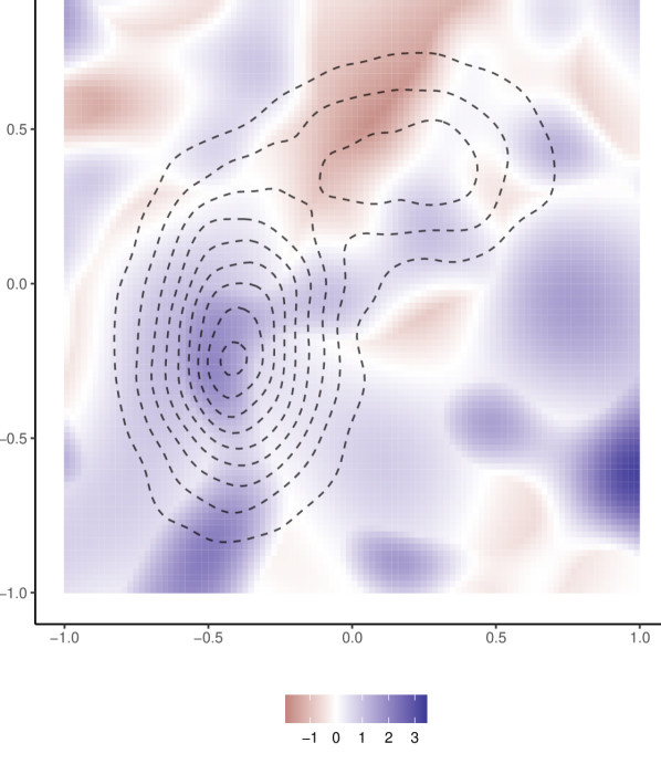


For each setting, we set the distribution of to be a 2-component mixture of multivariate normal distributions, , where and are the same as in (18). Given the and , we generate the and by adding Gaussian errors in the same way as in Example 3-1. We fix , and consider different values of , where and . The performance metric ISE is computed via a uniform grid on the union of two rectangular regions, . From the distribution of , in the area outside these two rectangular regions, there are too few training ’s to learn the function correctly, regardless of which methods to use. We exclude such “non-informative” area, so that the ISE is informative for comparing differeing methods. In NNME, we use 10 layers in the network for representing and 6 layers in the network for approximating the posterior distribution of , with 32 nodes per layer. How to choose the model for was discussed in Section 2.4, and the recommendation is to use either the NICE model or a mixture model that has a sufficient number of components. Here we consider both options: NNME_NICE uses the NICE model, and NNME_GM4 models by a 4-component Gaussian mixture distribution with unknown parameters. We compare the two versions of NNME with the two kriging methods, KILE and KALE. The results are in Table 7.
| 500 | 1000 | 2000 | 4000 | 8000 | ||
|---|---|---|---|---|---|---|
| KILE | .415 (.021) | .349 (.019) | .280 (.015) | - | - | |
| KALE | .414 (.021) | .335 (.019) | .259 (.015) | - | - | |
| NNME_GM4 | .455 (.027) | .364 (.024) | .258 (.018) | .167 (.019) | .108 (.009) | |
| NNME_NICE | .483 (.049) | .398 (.039) | .250 (.020) | .202 (.033) | .124 (.014) | |
| KILE | .773 (.040) | .711 (.038) | .682 (.042) | - | - | |
| KALE | .809 (.040) | .748 (.038) | .714 (.042) | - | - | |
| NNME_GM4 | .820 (.081) | .696 (.066) | .548 (.037) | .389 (.024) | .313 (.027) | |
| NNME_NICE | .815(.065) | .670 (.058) | .459 (.050) | .429 (.045) | .350 (.035) | |
| KILE | .226 (.020) | .187 (.019) | .150 (.009) | - | - | |
| KALE | .232 (.020) | .187 (.019) | .147 (.009) | - | - | |
| NNME_GM4 | .251(.027) | .169 (.019) | .116 (.009) | .079 (.005) | .076 (.009) | |
| NNME_NICE | .303 (.030) | .175 (.022) | .140 (.013) | .103 (.013) | .072 (.010) | |
| KILE | .376 (.037) | .362 (.037) | .351 (.034) | - | - | |
| KALE | .382(.037) | .371( .037) | .363 (.034) | - | - | |
| NNME_GM4 | .400 (.042) | .321(.028) | .268 (.035) | .192 (.027) | .159 (.018) | |
| NNME_NICE | .442 (.042) | .367 (.052) | .300 (.055) | .241 (.039) | .181 (.021) |
The data generating process in the first setting is exactly the same as what KALE assumes, and one would expect KALE to perform the best. This is true when the measurement error is relatively small () or the sample size is small to moderate (). However, when the measurement error is large () or the sample size is , NNME outperforms KALE. Additionally, between the two versions of NNME, NNME_NICE has a better performance in this setting. We note that the two kriging methods, KILE and KALE, require computing the inverse of an matrix. Therefore, they do not scale to large . In fact, we are not able to run these methods for . In the second setting, is from the maximum of two Gaussian processes, and it is no longer the model assumed by the kriging methods. NNME uniformly outperforms KILE and KALE when . Between the two versions of NNME, NNME_GM4 is better in this setting.
We also investigated many similar settings with generated from 2-dimensional Gaussian processes, where we varied the RBF kernel and the distribution of measurement errors. A common observation is that the advantage of NNME, compared with kriging methods, is primarily in the cases where the sample size is large and the measurement error is moderate to large. If the sample size is too small (e.g., ) or the measurement error is too small, NNME may have the over-fitting issue and tends to under-perform KILE and KALE (these kriging methods have fewer parameters to estimate and no over-fitting issues). In such cases, it is recommended to increase the L2-regulation parameters in NNME to counter overfitting.
3.5 Summary and discussions
The numerical studies reveal several appealing properties of the neural network approach for estimating MEMs. The first is the flexibility of accommodating various kinds of . This is because deep neural networks have the ability of representing a variety of function classes. In the simulations, we find that NNME has a reasonably good performance in almost all settings, provided that the decoder network has 7 or more layers. However, classical nonparametric/semi-parametric methods have unsatisfactory performance when is non-smooth (Example 2).
The second is its insensitivity to variation of tuning parameters and network structures. Classical methods require choosing the bandwidth or knots. Inappropriate choices will lead to oversmoothing or undersmoothing. Hence, tuning parameter selection crucially affects their performances. We tested a few data-driven tuning parameter selectors, such as the method in Delaigle and Hall, (2008) that uses SIMEX to select bandwidth in the local polynomial deconvolution method, but they worked unsatisfactorily. For the neural network approach, parameters to select include the L2 regularization parameters and the network structure (e.g., how many layers in the encoder/decoder and how many nodes per layer). The performance is relatively insensitive to these parameters. We often fix the L2 regularization parameter (e.g., or ) in simulations, and it works universally well. For the choice of the network structure, we find that the algorithm’s performance is always similar as long as the decoder network has 7 or more layers.
The third is the convenience of implementation for dimension . In principle, one can extend most classical methods from to . However, several challenges remain: How to select the -dimensional bandwidth matrix or the knots of -dimensional splines? How to compute the solution? (Take the spline approach for example: The number of spline bases grows exponentially fast with , posting a big challenge on computation.) Even for it is hard to implement most classical methods. In contrast, the neural network approach can easily handle .
The last, but not the least, is the scalability to large sample size . For example, in Experiment 3, there are no other methods that can be implemented for , but the neural network approach can handle or even larger with ease. This is because the gradient ascent algorithm, and the back prorogation algorithm for computing gradients, is very fast.
On the other hand, the neural network approach is not a panacea. Its main limitation is the lack of theoretical guarantee. The elegant theory for classical methods tell us when those methods are consistent and what their rates of convergence are (Fan and Truong,, 1993; Delaigle et al.,, 2009; Jiang et al.,, 2018). For the neural network approach, so far we can only evaluate its performance numerically. Some limited theoretical understanding includes Kohler and Mehnert, (2011), where they study a special least-squares neural network estimator and show that its rate of convergence with error-in-variables is similar to the rate of convergence in the error-free case, when the measurement error is small. However, their neural network estimator is a simple one that ignores measurement error, and their theory does not cover the case where measurement error is large, for which NNME has the most appealing empirical performance.
4 Real Data Applications
We apply the NNME algorithm in two real data examples, the sea level study and the Framingham heart study.
4.1 Sea level data
The sea level studies model the change of sea levels in the past and predict the sea levels in the future. The data set in Kemp et al., (2011) consists of measurements of relative sea level (RSL) in North Carolina for the past 2000 years. The measurements were constructed from cores of coastal sediment, where ages of discrete depths in the core were estimated from radiocarbon dating and had uncertainty. Following Cahill et al., (2015), we use a measurement error framework to account for age uncertainty. Let be the observed RSL, the true calendar year, and the estimated calendar year (by fitting the radiocarbon dates with an age-depth model). Suppose the ocean level is . The true RSL is defined as the difference between ocean level and land level. According to the glacio-isostatic adjustment, the land level decreases at an annual rate of , where is given.111The value of varies with geographical locations. This dataset was measured at two sites, where and , respectively. Then, the model is
| (20) |
where the calendar years and have been divided by 1000 (e.g., 1996 is written as 1.996) and is the land level in 2010 AD. Both and are assumed to follow normal distributions:
| (21) |
where and are known for each observation. The data are . The goal is estimating the function . Without loss of generality, we let , so that the ocean level in 2010 AD is viewed as the baseline.
This problem is easily cast as a nonparametric regression with measurement errors. Write . We first apply NNME to estimate and then convert it to an estimate of straightforwardly. A minor difference from the previous MEMs is that the variance of response errors and measurement errors are both heterogeneous across observations. However, since and are known, our algorithm can be easily extended to this case. We incorporate into the marginal likelihood according to model (20)-(21), and modify the gradient ascent steps accordingly. These modifications are straightforward and omitted. We also modify (16) to an estimate of as
where are importance samples for the th observation and is ratio between the complete likelihood and the density of proposal distribution, similar to that in (16). We use a parametric model for , which is a 2-component mixture of Gamma distributions with unknown parameters. For the neural network structure, we let the decoder and encoder have 5 and 3 hidden layers, respectively, with 32 nodes per layer. We use tanh as the activation function in the decoder (to make smooth) and ReLU in the encoder. Since the variances of measurement errors are small (from to ) compared to the variance of calendar years (about ), we also add a direct link from to in Figure 1 to accelerate the learning process. It means the output of encoder becomes , where is from a 3-layer FNN. Besides an estimate of , we also compute a 95% confidence band via a parametric bootstrap procedure. In the standard model-based bootstrap, we should draw samples from the estimated model for and model (20)-(21) for . However, the noise variances in covariates and responses are only know at observed sites, and so we cannot use the standard model-based bootstrap. We instead fix , the estimated posterior mean of from the encoder, and draw from model (20)-(21) using the known variances for the th observation. The resulting bootstrap confidence band can be viewed as conditioning on (estimates of ) ’s.
The left panel of Figure 7 shows the estimated ocean level, which is . The right panel shows the estimated sea level change, which is the derivative of . It is computed by a back propagation algorithm using estimated parameters. The confidence band of is from a similar bootstrap procedure. We compare NNME with the approach in Cahill et al., (2015), denoted as “GP”, which models the sea level change (i.e., derivative of ) by a Gaussian process with measurement errors and uses Markov chain Monte Carlo for estimation and inference. While it is based on Gaussian process, this method is different from KALE. The estimated curves of sea level (left panel of Figure 7) by NNME and GP are similar, except in the period between 1600 AD and 1800 AD. Both methods estimate the sea level to decrease first and increase later in this period, but NNME estimates this “fluctuation” be less prominent. For GP, we plot the 95% Bayesian credible interval (Cahill et al.,, 2015). Although the credible interval is not directly comparable with the confidence band, we may still draw the conclusion from the plots that NNME gives less “confidence” on the fluctuation of sea level between 1600 AD and 1800 AD. The estimated curves of sea level change (right panel of Figure 7) are also similar. The curve by GP is smoother. A possible explanation is that GP directly models the sea level change while NNME models the sea level.


Since there is no ground truth, we compare the performance of different methods using prediction errors. Given and a testing , we predict by , where the expectation is with respect to the posterior distribution of given . We use two ways to approximate the posterior distribution of . The first is , where is the variance of measurement errors in this observation. This ad-hoc approach can be viewed as imposing a flat prior on . The second is using the estimated prior distribution of from NNME to derive the posterior distribution of . In the actual implementation, to obtain , we first draw samples from the prior distribution of and then take a weighted average of , with weights proportional to the conditional likelihood of given . For each , we construct predictors using both ways. We measure the prediction performance using a cross-leave-out procedure: We randomly partition data into 5 folds, successively use each fold for testing (with the other 4 folds as training data) and compute the mean-squared-error. We then take the average of 5 mean-squared-errors and use it as the prediction error. We repeat this procedure for 10 times and report the mean and standard error of the prediction error. The results are as follows:
| NNME_posterior1 | NNME_posterior2 | GP_posterior1 | GP_posterior2 | NN |
| 1.387 (0.068) | 1.402 (0.069) | 1.499 (0.065) | 1.503 (0.065) | 2.478 (0.020) |
NNME is better than GP in terms of prediction performance. We also report the prediction error by NN; it ignores measurement errors in estimating and predicts by . The performance of NN is much worse than NNME, suggesting that the advantage of NNME comes from not only using neural networks but also accounting for measurement errors.
4.2 Framingham Heart Study
The Framingham Heart Study is an ongoing cardiovascular study on residents of the town of Framingham, Massachusetts. The goal of this study is to predict whether the patient will have coronary heart disease (CHD) in 10 years. The dataset includes over 4,000 records and 15 attributes of patients including demographic, behavioral and medical risk factors. We downloaded the data set from Kaggle222https://www.kaggle.com/dileep070/heart-disease-prediction-using-logistic-regression.. The covariate of particular interest is the systolic blood pressure (SBP). However, it is impossible to measure the long-term SBP directly, and the observation recorded is the blood pressure measured in a single clinic visit, which has considerable daily variations. The measurement error of the transformed SBP (i.e., log(SBP)) was assumed to be Gaussian whose variance was estimated by several clinic visits of the same patient. Other covariates were assumed error-free, except for the logarithm of the total cholesterol level (Chol). We followed Carroll et al., (2006) to model the measurement errors on SBP and Chol as bivariate Gaussian with a given covariance matrix. We proposed to fit a nonparametric logistic regression
where is the logistic sigmoid function, indicates whether or not this patient has CHD in 10 years, ’s are error-free covariates, and for only error-prone observations, , are available. Previous studies usually used a linear logistic regression model with measurement errors. In comparison, our approach can estimate the nonlinear, interaction effects on SBP and Chol.
We pre-processed data by dividing the variable age by 100 and then centering all variables to have mean zero. We then adapted NNME to the current setting by changing the form of the log-likelihood. We estimated coefficients of other variables by jointly maximizing the IWAE objective via gradient ascent (again, we used the doublely reparametrized gradient estimator for parameters in the encoder). We used 3 hidden layers for both the decoder and encoder, with 32 nodes per layer and ReLU as the activiation function. To cope with the logistic model, we used the sigmoid function in the last layer of the decoder. We used NICE to model the (prior) joint distribution of SBP and Chol. The estimated 10-year risk of CHD, as a 2-dimensional function of SBP and Chol, is shown in Figure 8.

We compared NNME with the method SIMEX. SIMEX has to base on a nonparametric logistic regression method that ignores measurement errors; we used penalized splines (degree = 2, number of knots = 10). 333It is common to use quadratic extrapolation in SIMEX. However, on this data set, quadratic extrapolation is considerably worse than linear extrapolation. Therefore, we reported results of linear extrapolation. The code to implement SIMEX basically allows for only 1 error-prone covariate; to apply it to 2 error-prone covariates, we have to assume an additive model. Consequently, this approach does not model interaction effects between SBP and Chol. In contrast, NNME includes a bivariate function of SBP and Chol in the risk and is able to capture interaction effects. Previously in Section 3, we also considered KALE for 2 error-prone covariates; unfortunately, KALE has no direct extension to the logistic regression model. The estimated 10-year risks of CHD by NNME and SIMEX are shown in Figure 8. For a better comparison, we also considered two methods that ignore measurement errors, NN and Pspline, as counterparts of NNME and SIMEX. See Figure 8. The comparison of risk contours of Pspline versus NN suggests that neural neworks can capture nonlinear effects (beyond quadratic ones) of both SBP and Chol, as well as the interaction effect between two covariates. SIMEX generates more sophisticated risk contours than Pspline, but SIMEX still does not model interaction effects. NNME is the only one among 4 methods that accommodates measurement errors, nonlinear effects, and interaction effects.
To check whether NNME overfits, we evaluated the classification performance. Given an estimated model, we classify a sample by thresholding , where the posterior distribution of is obtained from the measurement error distribution and the prior distribution from NICE. To avoid discussion of thresholds, we measure the performance by the area under ROC curve (AUC). We randomly selected 20% of CHD samples and 20% of non-CHD samples for testing and used the remaining samples for training. The mean and standard deviation of AUC, over 20 random splits of training and testing, are:
| Pspline | SIMEX | NN | NNME |
| 0.727 (0.005) | 0.728 (0.005) | 0.727 (0.005) | 0.728 (0.005) |
The AUCs of different methods are similar. At least, it suggests that the more sophisticated models from neural networks are not due to overfitting. Additionally, accounting for measurement errors marginally improves the classification performance.
5 Discussion
The use of neural networks in nonparametric statistics attracted a lot of recent attention, with encouraging progress on density estimation and nonparametric regression. This paper is an attempt to introduce neural networks to estimation of measurement error models, one of the classical topics in nonparametric statistics (Carroll and Hall,, 1988; Fan and Truong,, 1993; Carroll et al.,, 1999). We propose a neural network design, where the regression function , the (prior) distribution of , and the posterior distribution of given the error-prone covariates are represented by three different neural networks. We estimate parameters of these neural networks by maximizing an “importance sampling” lower bound of the marginal log-likelihood of . We solve the optimization by a stochastic gradient ascent algorithm, with a doubly reparametrized gradient estimator. Our algorithm combines recent advancements in neural network, including Burda et al., (2016) on variational auto-encoder, Tucker et al., (2018) on stochastic gradient descent, and Dinh et al., (2015) on normalizing flow.
Through extensive simulations and real data analysis, we demonstrated that the neural network approach is a promising alternative to classical nonparametric methods for MEMs. The neural network approach is flexible for accommodating various classes of functions (even non-smooth functions); its performance is insensitive to tuning parameters; it is convenient to implement for dimension ; and it has good scalability to a large sample size. Additionally, our method can be easily extended to more general settings. For example, if the noise in or the noise in is non-additive, our method can be implemented similarly, where we simply change the expression of the joint density of . In contrast, classical nonparametric methods are more restrictive on model assumptions; for example, the deconvolution method (Fan and Truong,, 1993) relies on that the measurement error is additive.
Theoretical understanding of neural network methods is a trending topic. Many theoretical frameworks were proposed, such as size-independent complexity (Bartlett,, 1998; Golowich et al.,, 2018), implicit regularization (Soudry et al.,, 2018), seive approximation (Chen and White,, 1999), mean-field approximation (Mei et al.,, 2018), and so on. Whether or not these theoretical frameworks can be used to understand the behavior of our method for MEMs is an open problem. We leave it for future work.
Appendix
Appendix A Variational inference versus maximizing likelihood
The neural network method we propose for MEMs adopts the variational inference framework, where parameters are estimated by maximizing an evidence lower bound (ELBO) of the marginal log-likelihood. In this appendix we consider a different approach, that is, maximizing the joint likelihood of , with respect to both model parameters and unobserved values of ’s (MJL, henceforth). Same as before, we use an FNN to represent the regression function . Next, we use another FNN to approximate the “most likely” estimate of given the observed data, i.e.,
| (22) |
where contains parameters of this FNN, which will be determined jointly by . We then write down the joint likelihood as (following the convention, we only present it for ; the extension to a general is straightforward):
| (23) |
The parameters are estimated by maximizing . The neural network structure that implements this estimator is shown in Figure 9.

In comparison, the variational inference framework approximates the posterior distribution of by and maximizes an integral with respect to this distribution, which serves as a lower bound of the marginal log-likelihood. See equation (7).
We compare the “maximizing joint likelihood” framework and the variational inference framework. For a fair comparison, we use the basic variational inference approach, where the number of importance samples is . It corresponds to the method VAE in Table 1. We solve both the MJL and VAE by the gradient ascent algorithm, where the gradient of (23) is computed directly, the gradient for VAE is estimated as in (11) with , and the step size for both is chosen by Adam (Kingma and Ba,, 2014). The noise variance is optimized together with , similarly as in Section 2.3.


We consider the simulation setting of Experiment 1 of Section 2.4, where is the true regression function. The errors of MJL and VAE were already reported in Figure 2(a). These results suggest that the variational inference framework is better than the “maximizing joint likelihood” framework, especially when is small or moderate. Intuitively the MJL framework “imputes” the “missing data" to maximize the joint likelihood, whereas the VAE approaches marginalizing the “missing data” like in the EM algorithm, but based on a slightly incorrect distribution. In Figure 10 we plot the estimated curves by MJL and VAE, where and . At each where reaches a local maximum or minimum, the estimated curve by MJL has a bias in the neighborhood of . This is because that MJL fails to take into account the uncertainty of given . Intuitively, in MJL is determined only by those such that , while in VAE is determined by more corresponding to a wider range of . As a result, when reaches a local minimum or maximum, it is likely to have extreme values of , and even a few such can drag to be extreme in MJL; this will not happen in VAE because an individual value of is less influential.
Appendix B Comparison of models for in NNME
The proposed method, NNME, is flexible to accommodate different kinds of models (prior distributions) for . In Experiment 3 of Section 2.4, we tested 4 variants of NNME, where the model for is either the correct parametric model (2-component Gaussian mixture), or a misspecified parametric model (t-distribution, or 4-component Gaussian mixture), or a neural network model (NICE).
The data generation in this experiment is as follows: Fixing , we generate from a 2-dimensional Gaussian processes as in (19). In detail, we first generate from the distribution of , which is a 2-component mixture of multivariate Gaussian distributions as in (18). Next, we construct an covariance matrix , with , and then generate from .

In Section 2.4 we have reported the results for a few values of model parameters. Here we investigate more settings. We let the sample size range in and let the measurement error standard deviation range in . We also vary the neural network structures: Let be the number of layers of the two FNNs for representing and the posterior distribution of , respectively. We let range in . The performance is measured by the integrated squared error (ISE) in the region ; according to the distribution of in (18), the probability of ’s falling outside this region is negligible, and so we restrict the error evaluation to be in this region. The results are shown in Figure 11, demonstrating that NNME performs robustly with different choices of the model when is small, but shows superiority with NICE or 4-component Gaussian mixture when is large.
Appendix C Sensitivity to the depth of neural networks
As we stated in Section 1, the neural network approach to MEMs is relatively insensitive to the choice of tuning parameters. Main tuning parameters include the depth of the two FNNs for representing and the posterior distribution of . We now investigate the sensitivity of NNME to the depth of neural networks.

We consider a simulation setting where the ’s are drawn uniformly from and the ’s are generated from a Gaussian process as in (19) with (see Section 3.4 or Appendix B for details about generating data from a Gaussian process). The measurement errors are drawn from . For a set of values of , we study the performance of NNME by varying the depth of neural networks. We place hidden layers in the decoder (for representing ) and hidden layers in the encoder (for approximating the posterior distribution of ), where each layer has 32 nodes with ReLU activation functions; the encoder has an additional layer with linear activation functions. We let range in and range in . The integrated squared error (ISE) is evaluate using a grid.
The results are shown in Figure 12. For most values of , as long as the depth of neural networks satisfies and , the performance is reasonably good. The only exceptions are when the sample size is small (e.g., ) or when the measurement error is large (e.g., ). In such cases, we will see that a procedure like cross validation can select the appropriate number of layers.


We then investigate the selection of depth of neural networks by two criteria. The first is the validation loss we eventually used, which is the weighted residual sum of squares in (16), evaluated on the validation data. To compute this quantity, we need to use estimated parameters from the training data and draw new Monte Carlo samples ; see Section 2.3 for details. We call this criterion the “estimated RSS.” The second is the loss function (7) in NNME algorithm, evaluated on the validation data. It is an evidence lower bound (ELBO) of the marginal log-likelihood. Again, to obtain an approximation to this quantity, we need to use the fitted parameters from the training data and also draw new Monte Carlo samples . We call it the “estimated ELBO.” For both criteria, we calculate the 5-fold cross-validation version. Figure 13 shows the values for different choices of depth of neural networks.
We compare these criteria with the true ISE in Figure 12. As we change the depth of neural networks, the trend in the estimated RSS roughly matches with the trend in the true ISE. Especially, as we mentioned above, if the sample size is small (e.g., ) or the measurement error is large (e.g., and ), it is not always good to increase the depth of neural networks. In these cases, the cross-validation procedure, with the estimated RSS as the validation loss, can successfully guide us to the appropriate choice of depth. The other criterion, the estimated ELBO, is a lot more sensitive to the parameters and tends to select a larger number of layers for the encoder. In comparison, the estimated RSS we used in Section 2.3 is a better option for the validation loss.
References
- Barron, (1993) Barron, A. R. (1993). Universal approximation bounds for superpositions of a sigmoidal function. IEEE Transactions on Information theory, 39(3):930–945.
- Bartlett, (1998) Bartlett, P. L. (1998). The sample complexity of pattern classification with neural networks: the size of the weights is more important than the size of the network. IEEE Transactions on Information Theory, 44(2):525–536.
- Bauer and Kohler, (2019) Bauer, B. and Kohler, M. (2019). On deep learning as a remedy for the curse of dimensionality in nonparametric regression. The Annals of Statistics, 47(4):2261–2285.
- Berry et al., (2002) Berry, S. M., Carroll, R. J., and Ruppert, D. (2002). Bayesian smoothing and regression splines for measurement error problems. Journal of the American Statistical Association, 97(457):160–169.
- Burda et al., (2016) Burda, Y., Grosse, R., and Salakhutdinov, R. (2016). Importance weighted autoencoders. In International Conference on Learning Representations.
- Cahill et al., (2015) Cahill, N., Kemp, A. C., Horton, B. P., and Parnell, A. C. (2015). Modeling sea-level change using errors-in-variables integrated gaussian processes. The Annals of Applied Statistics, 9(2):547–571.
- Carroll et al., (1999) Carroll, R., Maca, J., and Ruppert, D. (1999). Nonparametric regression in the presence of measurement error. Biometrika, 86(3):541–554.
- Carroll and Hall, (1988) Carroll, R. J. and Hall, P. (1988). Optimal rates of convergence for deconvolving a density. Journal of the American Statistical Association, 83(404):1184–1186.
- Carroll et al., (2006) Carroll, R. J., Ruppert, D., Stefanski, L. A., and Crainiceanu, C. M. (2006). Measurement error in nonlinear models: a modern perspective. Chapman and Hall/CRC.
- Chen and White, (1999) Chen, X. and White, H. (1999). Improved rates and asymptotic normality for nonparametric neural network estimators. IEEE Transactions on Information Theory, 45(2):682–691.
- Cook and Stefanski, (1994) Cook, J. R. and Stefanski, L. A. (1994). Simulation-extrapolation estimation in parametric measurement error models. Journal of the American Statistical Association, 89(428):1314–1328.
- Cressie and Kornak, (2006) Cressie, N. and Kornak, J. (2006). Spatial statistics in the presence of location error with an application to remote sensing of the environment. Statistical Science.
- Delaigle et al., (2009) Delaigle, A., Fan, J., and Carroll, R. J. (2009). A design-adaptive local polynomial estimator for the errors-in-variables problem. Journal of the American Statistical Association, 104(485):348–359.
- (14) Delaigle, A. and Gijbels, I. (2004a). Bootstrap bandwidth selection in kernel density estimation from a contaminated sample. Annals of the Institute of Statistical Mathematics, 56(1):19–47.
- (15) Delaigle, A. and Gijbels, I. (2004b). Practical bandwidth selection in deconvolution kernel density estimation. Computational Statistics & Data Analysis, 45(2):249–267.
- Delaigle and Hall, (2008) Delaigle, A. and Hall, P. (2008). Using SIMEX for smoothing-parameter choice in errors-in-variables problems. Journal of the American Statistical Association, 103(481):280–287.
- Dinh et al., (2015) Dinh, L., Krueger, D., and Bengio, Y. (2015). NICE: Non-linear independent components estimation. In Workshop in International Conference on Learning Representations.
- Eilers and Marx, (1996) Eilers, P. H. and Marx, B. D. (1996). Flexible smoothing with B-splines and penalties. Statistical science, pages 89–102.
- Fan et al., (2020) Fan, J., Ma, C., and Zhong, Y. (2020). A selective overview of deep learning. Statistical Science (to appear).
- Fan and Truong, (1993) Fan, J. and Truong, Y. K. (1993). Nonparametric regression with errors in variables. The Annals of Statistics, 21(4):1900–1925.
- Golowich et al., (2018) Golowich, N., Rakhlin, A., and Shamir, O. (2018). Size-independent sample complexity of neural networks. In Conference On Learning Theory, pages 297–299.
- Hall and Qiu, (2005) Hall, P. and Qiu, P. (2005). Discrete-transform approach to deconvolution problems. Biometrika, 92(1):135–148.
- Hecht-Nielsen, (1992) Hecht-Nielsen, R. (1992). Theory of the backpropagation neural network. In Neural Networks for Perception, pages 65–93. Elsevier.
- Jiang et al., (2018) Jiang, F., Ma, Y., and Carroll, R. J. (2018). A spline-assisted semiparametric approach to non-parametric measurement error models. arXiv preprint arXiv:1804.00793.
- Jordan et al., (1999) Jordan, M. I., Ghahramani, Z., Jaakkola, T. S., and Saul, L. K. (1999). An introduction to variational methods for graphical models. Machine Learning, 37(2):183–233.
- Kemp et al., (2011) Kemp, A. C., Horton, B. P., Donnelly, J. P., Mann, M. E., Vermeer, M., and Rahmstorf, S. (2011). Climate related sea-level variations over the past two millennia. Proceedings of the National Academy of Sciences, 108(27):11017–11022.
- Kingma and Ba, (2014) Kingma, D. P. and Ba, J. (2014). Adam: A method for stochastic optimization. In International Conference on Learning Representations.
- Kingma and Welling, (2014) Kingma, D. P. and Welling, M. (2014). Auto-encoding variational bayes. In International Conference on Learning Representations.
- Kohler and Mehnert, (2011) Kohler, M. and Mehnert, J. (2011). Analysis of the rate of convergence of least squares neural network regression estimates in case of measurement errors. Neural Networks, 24(3).
- Le et al., (2018) Le, T. A., Igl, M., Rainforth, T., Jin, T., and Wood, F. (2018). Auto-encoding sequential Monte Carlo. In International Conference on Learning Representations.
- Liang, (2018) Liang, T. (2018). On how well generative adversarial networks learn densities: Nonparametric and parametric results. arXiv preprint arXiv:1811.03179.
- Lin et al., (2017) Lin, H. W., Tegmark, M., and Rolnick, D. (2017). Why does deep and cheap learning work so well? Journal of Statistical Physics, 168(6):1223–1247.
- Liu, (2008) Liu, J. S. (2008). Monte Carlo strategies in scientific computing. Springer Science & Business Media.
- Maiorov and Meir, (2000) Maiorov, V. and Meir, R. (2000). On the near optimality of the stochastic approximation of smooth functions by neural networks. Advances in Computational Mathematics, 13(1):79–103.
- McClelland et al., (1986) McClelland, J. L., Rumelhart, D. E., and Group, P. R. (1986). Parallel distributed processing. Explorations in the Microstructure of Cognition, 2:216–271.
- Mei et al., (2018) Mei, S., Montanari, A., and Nguyen, P.-M. (2018). A mean field view of the landscape of two-layer neural networks. Proceedings of the National Academy of Sciences, 115(33):E7665–E7671.
- Mhaskar, (1996) Mhaskar, H. N. (1996). Neural networks for optimal approximation of smooth and analytic functions. Neural Computation, 8(1):164–177.
- Papamakarios et al., (2017) Papamakarios, G., Pavlakou, T., and Murray, I. (2017). Masked autoregressive flow for density estimation. In Advances in Neural Information Processing Systems, pages 2338–2347.
- Rainforth et al., (2018) Rainforth, T., Kosiorek, A., Le, T. A., Maddison, C., Igl, M., Wood, F., and Teh, Y. W. (2018). Tighter variational bounds are not necessarily better. In International Conference on Machine Learning, pages 4277–4285.
- Rasmussen, (2003) Rasmussen, C. E. (2003). Gaussian processes in machine learning. In Summer School on Machine Learning, pages 63–71. Springer.
- Rezende and Mohamed, (2015) Rezende, D. and Mohamed, S. (2015). Variational inference with normalizing flows. In International Conference on Machine Learning, pages 1530–1538.
- Rezende et al., (2014) Rezende, D. J., Mohamed, S., and Wierstra, D. (2014). Stochastic backpropagation and approximate inference in deep generative models. In International Conference on Machine Learning, pages 1278–1286.
- Roeder et al., (2017) Roeder, G., Wu, Y., and Duvenaud, D. K. (2017). Sticking the landing: Simple, lower-variance gradient estimators for variational inference. In Advances in Neural Information Processing Systems, pages 6925–6934.
- Rolnick and Tegmark, (2018) Rolnick, D. and Tegmark, M. (2018). The power of deeper networks for expressing natural functions. In International Conference on Learning Representations.
- Schmidt-Hieber, (2017) Schmidt-Hieber, J. (2017). Nonparametric regression using deep neural networks with relu activation function. arXiv preprint arXiv:1708.06633.
- Singh et al., (2018) Singh, S., Uppal, A., Li, B., Li, C.-L., Zaheer, M., and Póczos, B. (2018). Nonparametric density estimation with adversarial losses. In International Conference on Neural Information Processing Systems, pages 10246–10257.
- Soudry et al., (2018) Soudry, D., Hoffer, E., Nacson, M. S., Gunasekar, S., and Srebro, N. (2018). The implicit bias of gradient descent on separable data. The Journal of Machine Learning Research, 19(1):2822–2878.
- Staudenmayer and Ruppert, (2004) Staudenmayer, J. and Ruppert, D. (2004). Local polynomial regression and simulation-extrapolation. Journal of the Royal Statistical Society: Series B (Statistical Methodology).
- Stefanski and Carroll, (1990) Stefanski, L. A. and Carroll, R. J. (1990). Deconvolving kernel density estimators. Statistics, 21(2):169–184.
- Tabak and Turner, (2013) Tabak, E. G. and Turner, C. V. (2013). A family of nonparametric density estimation algorithms. Communications on Pure and Applied Mathematics, 66(2):145–164.
- Titsias and Lázaro-Gredilla, (2014) Titsias, M. and Lázaro-Gredilla, M. (2014). Doubly stochastic variational bayes for non-conjugate inference. In International Conference on Machine Learning, pages 1971–1979.
- Tucker et al., (2018) Tucker, G., Lawson, D., Gu, S., and Maddison, C. J. (2018). Doubly reparameterized gradient estimators for Monte Carlo objectives. In International Conference on Learning Representations.
- Zhang et al., (2017) Zhang, C., Bengio, S., Hardt, M., Recht, B., and Vinyals, O. (2017). Understanding deep learning requires rethinking generalization. In International Conference on Learning Representations.