Mean-Square Input-Output Stability and Stabilizability of a Networked Control System with Random Channel Induced Delays
Abstract
This work mainly investigates the mean-square input-output stability and stabilizability for a single-input single-output (SISO) networked linear feedback system. The control signal in the networked system is transmitted over an unreliable channel. In this unreliable channel, the data transmission times, referred to as channel induced delays, are random values and the transmitted data could also be dropout with certain probability. The channel induced delays and packet dropout are modeled by an independent and identically distributed (i.i.d.) stochastic process with a fixed probability mass function (PMF). It is assumed that the transmitted data are with time stamps. At the channel terminal, a linear combination of data received at one sampling time is applied to the plant of the networked feedback system as a new control signal. To describe the uncertainty in the channel, a concept so called frequency response of variation is introduced for the unreliable channel. With the given linear receiving strategy, a mean-square input-output stability criterion is established in terms of the frequency response of variation of the unreliable channel for the networked feedback system. It is shown by this criterion that the mean-square input-output stability is determined by the interaction between the frequency response of variation and the nominal feedback system. In the mean-square input-output stability of the system, the role played by the random channel induced delays is the same as that played by a colored additive noise in an additive noise channel with a signal-to-noise ratio constraint. Moreover, the mean-square input-output stabilizability via output feedback is studied for the networked system. When the plant in the networked feedback system is minimum phase, an analytic necessary and sufficient condition is presented for its mean-square input-output stabilizability. It turns out that the stabilizability is only determined by the interaction between the frequency response of variation of the channel and unstable poles of the plant. Finally, numerical examples are given to illustrate our results.
1 Introduction
Networked feedback control systems are known as spatially distributed control systems in which signals are exchanged over communication network [1]. In the past few decades, a huge amount of research interests has been attracted on the analysis and design of these systems due to great advantages in networked control systems, such as ease for installation and maintenance, reduced system wiring, and resources sharing etc. Typical application examples of networked control systems can be found in a broad range of areas such as: automotive industry [2], autonomous underwater vehicles and unmanned air vehicles [3, 4], and even remote surgery [5] and big data [6]. Despite of the advantages, networked control systems also pose challenging problems arising from unreliability in data transmission, caused by channel induced delays (i.e., data transmission times), packet dropout, coding error etc. Due to the fact that data are transmitted in network by data packet, channel induced delays and data packet dropout that occur in data exchanging between components of feedback systems over network are the most common phenomena in networked systems. The channel induced delays and packet dropout could seriously degrade performance of feedback control systems, and even destabilize feedback systems when these issues are not carefully considered in system design (see, e.g., [7, 8] and [9]). To cope with channel induced delays, great efforts have been made in modeling, stability analysis, and controller design of networked feedback systems (for example see [7, 8] and the references therein).
Channel induced delays in networked systems could be constant, time-varying, and random delays, which are basically dependent on network protocol, channel quality etc. In [10, 11, 12], the authors studied the asymptotic stability of networked linear feedback systems in which message is transmitted over network with a constant transmission time (i.e. a constant channel induced delay). The networked systems were modeled as discrete-time linear systems augmented from discretized plants, delay channel models and control laws. In particular, the channel induced delay was modeled as a parameter of the augmented linear systems’ matrices. Stability criteria were obtained for the networked systems in terms of the discrete-time linear system models. These augmented models were also used to study the asymptotic stability and stabilization design for networked feedback systems with time-varying delays. Several stability criteria and stabilization design results were obtained by using switch system approaches (see for example [13, 14, 15, 16]). Alternatively, time-varying channel induced delays were modeled as continuous-time plants’ input delays (see e.g., [17, 18, 19]). Lyapunov-Krasovskii functionals were used in stability analysis and stabilization design for networked feedback systems. Various linear matrix inequality (LMI) based methods were developed. Moreover, to cope with data disorder occurred in transmission, time-stamp scheme and logic zero-order hold were developed for the networked feedback systems [20, 21]. In general, the aims of aforementioned papers are to find criteria that networked feedback systems are stable when channel induced delays belong to given regions, or to find upper bounds of channel induced delays under which the stability of the networked feedback systems are preserved. This leads to certain conservativeness in stability analyses and stabilization design for networked feedback systems with random channel induced delays.
Since channel induced delays and packet dropouts usually exhibit random characteristics, random channel induced delay and packet dropout models are widely used in stability analysis and control design for networked feedback systems (see for example [22, 20, 23, 24, 25]). In [24, 25], applying Markov chains, the authors modeled networked systems with random delays and packet dropouts as discrete-time Markov jump linear systems. Necessary and sufficient conditions were obtained for the mean-square stability of the networked feedback systems. Then, the mean-square stabilization was studied for these systems and LMI based control design approaches were developed. It turned out that this stabilization problem is a non-convex problem. Certain conservativeness may not be avoidable in this type of results. On the other hand, channel induced delays were modeled as random input delays of plant/controllers, and the sequences of the input delays were assumed to be independent and identically distributed (i.i.d.) random processes in [22, 20]. It was assumed in these works that the probability density functions of the random channel induced delays are known and all the channel induced delays in networked feedback systems are smaller than the systems’ sampling intervals. A suboptimal linear controller was designed for a networked feedback system with a fixed sampling interval in [20]. The reference [22] studied a networked system with a time-varying sampling interval. LMI based sufficient conditions were presented for the mean-square stability of the system. However, for the case when channel induced delays are longer than the systems’ sampling intervals, the channel induced delays may not exactly be input delays of plants since more than one data may be received simultaneously or none data could be received at one sampling instant. In [26, 23, 27, 28], channel induced delays (or data transmission times) which are longer than the systems’ sampling intervals were modeled as an i.i.d. random process with a known probability mass function (PMF). State estimation problem was studied for these networked systems and optimal state estimation algorithms were developed in [27, 28]. The stabilization problem was studied for a nonlinear networked feedback system and a sufficient condition was obtained for the stability of the networked feedback system in [23].
In this work, we focus on a single-input single-output linear time-invariant (LTI) networked feedback system in which the control signal is transmitted over a communication channel with random channel induced delays. The networked feedback system is a discrete-time system with a fixed sampling interval and channel induced delays are integral multiples of this sampling interval. Our goal is to fully understand how the interaction between stochastic features of the random delays and characteristics of the networked feedback system affects the system’s stability and limits the stabilizability of the system. With these purposes, we adopt the random process model studied in [26, 23, 27, 28] to describe the random channel induced delays. At the channel terminal, a linear receiving strategy which is a linear combination with given weights of data received at one sampling time is adopted. The new signal generated by the linear receiving strategy is applied to the plant of the networked feedback system as a control signal. Then, the channel uncertainty caused by the random channel induced delays is defined by the random impulse response of the communication channel and the first-order statistics of the impulse response. The input-output relation of the channel uncertainty is established in terms of the spectral density of the uncertainty’s impulse response. To give a precise description for a channel relative deviation induced by the channel uncertainty, a concept of so-called frequency response of variation is introduced in frequency domain. A necessary and sufficient condition is presented for the mean-square input-output stability of the networked feedback system. It is a new version of the small gain theorem for networked feedback systems with random channel induced delays. It is also found that for the mean-square input-output stability and stabilizability problems, the channel uncertainty caused by the random channel induced delays is equivalent to an additive noise in an additive noise channel with a signal-to-noise ratio constraint (see [29] and [30] for more details in the mean-square stability of networked feedback systems over additive noise channels with a signal-to-noise ratio constraint). After then, the mean-square input-output stabilizability via output feedback is studied for the networked feedback system. In particular, a necessary and sufficient condition is found for the mean-square input-output stabilizability of the system when its plant is minimum phase. It precisely describes the connection between the mean-square input-output stabilizability, the frequency response of variation and the unstable poles of the plant in the feedback system. Furthermore, it turns out that the interaction between the frequency response of variation and the unstable poles plays a critical role to the mean-square stabilizability of the networked feedback system.
The remainder of this paper is organized as follows. In Section 2, the random channel induced delays and related channel uncertainty are modeled by using the PMF of the delays. The impulse responses of the channel and channel uncertainty are given. The problems under study are formulated. Section 3 presents the input-output relation of the channel uncertainty based on the spectral density of its impulse response. A necessary and sufficient condition of the mean-square input-output stability is obtained for the networked feedback system. In Section 4, the mean-square input-output stabilizability is studied for the networked feedback system when its plant is minimum phase. An analytic expression is obtained for the necessary and sufficient condition of the mean-square input-output stabilizability. The connection between the result in this work and the existing results is discussed. Section 5 illustrates some numerical examples and Section 6 concludes the paper.
The notations used in this paper is mostly standard. The complex conjugate transpose of any matrix is denoted by . When is square and invertible, its inverse and inverse conjugate transpose are denoted by and , respectively. For any transfer function , we represent a state-space realization of by . Let the open unit disc be denoted by , the closed unit disc by , the unit circle by , and the complements of and by and , respectively. In this work, the Hardy space consists of scalar-valued analytic function in such that
The orthogonal complement of is given by
Define also the space as the set of all proper stable rational transfer functions. Furthermore, denotes the expectation operator of a random variable. The set of real numbers is denoted by .
2 Problem Formulation
Consider a canonical structure of a discrete-time LTI networked feedback system as depicted in Fig. 1. Here, the plant is an LTI system and its transfer function is assumed to be strictly proper. The controller is an LTI controller.
The signal is the measurement of the plant , is the control signal generated by the linear controller , and is the external input. An unreliable communication channel is placed in the path from the controller to the receiver. Here, the unreliable features under study are random channel induced delays and packet dropout. Denote the channel induced delay for the control signal (i.e., the transmission time spent on transmitting over the communication channel) by . Thus, the signal sent at the time arrives at its destination at the time . The channel induced delay is assumed to be a random variable with nonnegative integer values from a bounded set . All transmitted data are with time stamps. The data whose channel induced delays are greater than are discarded at the receiver. is a collection of data, which has entries and includes all data received at time . Now, we use Kronecker delta function to characterize all entries belonging to ,
Let and . The function indicates that the signal arrives at its destination through the channel at time and , otherwise it means that is not received at time and . It is assumed that the receiver at the terminal of the channel has limited computation capability. This capability allows the receiver to generate the signal as its output based on the received data and the time stamps associated with the data. A linear combination of the received data can be taken as the output of the receiver:
| (1) |
where the weights are assigned to the received data, respectively, according to the delay steps of the data. We refer to the receiver given by (1) as linear receiver or linear receiving strategy. Note that the linear receiving strategy is a general case of the zero-input strategy [31]. Without loss of generality, we assume that the initial time is at and the system is at rest at initial time.
Remark 1.
For any given and a realization of , the indicator guarantees that the control signal could only appear in one element of the sequence . Being consistent with , the data appears in the sequence once at most. Moreover, to drop data with a channel induced delay greater than and model data dropout, the weight is set to be zero. That is, a zero-input strategy is adopted.
According to the discussion above, the networked feedback system in Fig. 1 with the linear receiver is re-diagrammed as that shown in Fig. 2, wherein is the unit delay operator.
One can see from this block-diagram that the block cascaded by the channel and the receiver, referred to as a transmission block, is a linear system with a random finite impulse response. Its input-output relation is given by (1). Since the initial time is assumed to be zero, without loss generality, we consider the random impulse response of the transmission block to a unit impulse input applied to the channel at any time , which is given by
| (2) |
One can see from (2) that the random impulse response is determined by the instant and the random sequence . For a given realization of , at most one entry is not equal to zero in the random sequence. The input-output relation of the transmission block is rewritten as
We impose the following assumptions throughout the paper.
Assumption 1.
The random delay process is an i.i.d. process, and takes values in according to a common PMF that
| (3) |
with and .
Assumption 2.
The external input sequence is independent of the channel induced delay process .
Since the random sequence is dependent on the random variable which is an entry of an i.i.d. process, the mean of each entry in this sequence is obtained from the PMF of , i.e.,
| (4) |
Define the mean channel as
Thus, it holds that
| (5) |
Subsequently, the transmission block is divided into two parts: One is the mean channel and the other is a zero-mean channel uncertainty denoted by . Denote the response of the latter part by to the unit impulse input applied to the channel at time . This impulse response is given as below:
| (6) |
Accordingly, the receiver output is the summation of the outputs of and when considering as their inputs, i.e.,
| (7) |
where
| (8) | ||||
| (9) |
As a result, the system in Fig. 2 can be re-diagramed as a stochastic system shown in Fig. 3. The structure of this system is similar to that studied in literatures for networked feedback systems over fading channels (see for example [32] and [33]). In the literatures, the channel uncertainties under study are white noise processes, thus the mean channels are constants and the channel uncertainties are zero-mean white noise processes. But, in this work, the mean channel and channel uncertainty are linear systems with the time-invariant finite impulse response and the random finite impulse response , respectively.
In Fig. 3, denote the system from to without considering the channel uncertainty by , referred to as the nominal system, which is given by
| (10) |
Then the whole system is an interconnection of the nominal system and the channel uncertainty , as shown in Fig. 4.
It is well-known that there exists a controller to internally stabilize the nominal feedback system for any stabilizable and detectable LTI plant if and only if there is not unstable pole-zero cancelation between the mean channel and the plant . That is, the following assumption is necessary.
Assumption 3.
The plant of the networked feedback system is stabilizable and detectable. There is not unstable pole-zero cancelation between the mean channel and the plant .
To avoid any possible unstable pole-zero cancelation, the weights , in the linear receiving strategy can also be selected so that the mean channel is minimum phase. A numerical example is presented in Section 5. Since the controller-receiver co-design is a very difficult task in general, a common setup in most of literatures is that the controller is designed based on a given receiving strategy, e.g., zero-input strategy or hold-input strategy for packet dropout problem [32, 31]. In this work, we restrict ourselves to the fixed weights of the linear receiving strategy such that is minimum phase. Throughout this paper, we concentrate on the mean-square input-output stability and stabilizability defined next.
Definition 1.
The channel induced delay process satisfies Assumption 1. The networked feedback system with a given linear receiving strategy shown in Fig. 2 is mean-square input-output stable if the linear controller internally stabilizes and the signal sequence is with bounded variances for any i.i.d. input process with a bounded variance and independent of the channel induced delay process.
Let the set of all proper controllers internally stabilizing be .
Definition 2.
The networked feedback system with a given linear receiving strategy shown in Fig. 2 is said to be mean-square input-output stabilizable via output feedback if there exists a feedback controller such that the closed-loop system is mean-square input-output stable.
Remark 2.
For a memoryless channel with a memoryless uncertainty, the channel model is given by
| (11) |
where is the mean of the channel gain and is an i.i.d. process with zero mean and finite variance . It is well-known (for example see [32, 34]) that the networked feedback system over an unreliable channel modeled by (11) is mean-square (input-output) stable if and only if is internally stable and
| (12) |
where is referred to as the relative standard deviation or coefficient of variation (see for example [35]) of the random variable . It is a measure to the variation of the uncertain channel’s gain. In this paper, since the channel uncertainty under study is with memory, it is much more complicated than that induced by an i.i.d multiplicative noise. A generalized version of the mean-square input-output stability criterion is studied for the networked feedback system.
3 Mean-square Input-output Stability
In this section, we study the criterion of mean-square input-output stability for the networked feedback system with a given output feedback controller . The frequency variable will be omitted whenever no confusion is caused.
It is shown in preceding section that a networked feedback system with a random channel induced delay and a linear receiver is modeled as a stochastic system shown in Fig. 3. Intuitively, the mean-square input-output stability of the system is determined by the interaction between the nominal feedback system and the zero-mean channel uncertainty . To study the interaction between and , the stochastic properties of the channel uncertainty whose impulse response is given in (6) are studied.
Lemma 1.
Suppose that the random delay process satisfies Assumption 1. Then it holds to the impulse response of the channel uncertainty that
-
1.
for and ,
-
2.
for ,
-
3.
for , , ,
Proof.
Remark 3.
According to the definition of in (6), it holds that for and , i.e., there are only non-zero elements in the response of to the impulse input . Thus, is the collection of all non-zero elements in the sequence . Furthermore, it holds that
Lemma 1 shows that for any given , the first- and second-order statistics of all elements in the non-zero subsequence are determined by the PMF of the transmission time and independent of . For (), the subsequences and are mutually independent. From the proof of this lemma, it can be verified that these stochastic properties holds for all .
Now the second order stochastic properties of are studied. For any given instant , let the autocorrelation of the subsequence be given by
| (13) |
Note the fact that for and . For the case , only the terms with in the summation of (13) may not be equal to zero. By letting , and applying Lemma 1.2 into (13), we obtain that
| (14) |
In the case when , note the fact that for any . It is verified by (13) that
Subsequently, define the energy spectral density of the channel uncertainty as follows:
| (16) |
Lemma 2.
The energy spectral density of the channel uncertainty can be written as
| (17) |
Proof.
Note the fact that any , . It holds that
Remark 4.
Note, from (14)-(15), that the autocorrelation of the subsequence is only dependent on the parameters of the transmission block (i.e., the PMF of the delay and the given weights in the receiving strategy) but independent of , so is the corresponding energy spectral density function given by (16). This allows us to establish the input-output relation of the channel uncertainty .
Lemma 3.
Proof.
Since the plant is assumed to be strictly proper, the controller output only depends on the past inputs of , which is determined by and , provided that and are relaxed at . Then by Assumptions 1 and 2, the current channel transmission time is independent of the current and past channel inputs, which completes the proof. ∎
Define the autocorrelation of the sequence by
| (21) |
It follows from (21) that
| (22) |
The power spectral density of is as follows:
| (23) |
Denote the th-component of in (9) by , , i.e.,
Lemma 4.
Proof.
For any stochastic sequence , denote its averaged power by ,
Lemma 5.
Proof.
The autocorrelation of is determined by the autocorrelations of its components . It follows from (9) that
| (28) | ||||
Applying Lemma 4 to (28) leads to
| (29) | ||||
For , it holds that
| (30) | ||||
According to Lemma 4, we write (30) as
| (31) |
Moreover, for any and , is independent of . It leads to
| (32) |
Remark 5.
As mentioned in the preceding section, an unreliable channel with random packet dropout can be modeled by a multiplicative white noise process with variance , and the variance is determined by the packet dropout probability (see [32, 33, 36, 37] and references therein). According to our framework, it holds for this case that , the mean channel is a constant determined by the packet dropout probability and the spectral density of the channel uncertainty is . For this white noise channel uncertainty, it holds that . It follows from Lemma 5 that
| (40) |
Moreover, it is not hard to verify that (40) holds for all channel uncertainties modeled by multiplicative white noises with zero mean and variance .
It is well-known that for spectral density , there exists a minimum phase polynomial of with degree and real coefficients satisfying
| (41) |
It is referred to as the spectral factorization of in literatures (see for example [38, 39]).
Notice the fact that and are real polynomials of with degree . The function
| (42) |
is, therefore, proper and real-rational. The complementary sensitivity function in the nominal system shown in Fig. 3 is given by
| (43) |
The next theorem establishes a new small gain theorem for mean-square input-output stability of the networked feedback system shown in Fig. 2.
Theorem 1.
Proof.
Consider the system in Fig. 4. Denote the power spectral densities of the signals , , and by , , and , respectively. Denote the autocorrelation of by . It holds for the averaged power and power spectral density of the signal that
| (45) |
and
| (46) |
It is well-known that for the linear system , the power spectral densities of its input signal and output signal satisfy
| (47) |
Hence, we obtain that
| (48) |
Since the input sequence is independent of , for any , and , and are mutually independent, is independent of . This leads to that
| (49) |
Consequently, we obtain that
| (50) |
Applying Lemma 5, we write (50) as
| (51) |
Substituting (51) into (48) leads to
| (52) | ||||
Taking account to the spectral factorization (41), we have that
| (53) |
The power exists if and only if .
Note that
This theorem holds. ∎
Remark 6.
In literatures (see for example [32] and references therein), there is a classical version of the mean-square small gain theorem for a networked feedback system over unreliable channel of which the channel uncertainty is modeled as a multiplicative white noise process. As shown by (12), the mean-square (input-output) stability of the system is determined by the interaction between the coefficient of variation of the unreliable channel’s gain and the complementary sensitivity function of the nominal system. Theorem 1 is a generalized version of this mean-square input-output stability criterion for the networked system with a random channel induced delay. As shown by the inequality (44), the mean-square input-output stability of the networked system is determined by the interaction between the factor and the complementary sensitivity function of the nominal system. In fact, is the coefficient of variation of the channel gain at the given frequency . Here, is referred to as the frequency response of variation of the channel.
To understand the role played by in data transmission, we consider the channel with a random channel induced delay shown in Fig. 3 where and are the mean channel and the channel uncertainty, respectively. Since the mean channel is a linear time-invariant system, the power spectral density of its output satisfies that
The power spectral density of the output of is given by Lemma 5. Thus, we obtain that
| (54) |
Note from the structure of the channel (or (7)) that the ratio is the signal-to-noise ratio (SNR) of the channel at the frequency and is the normalized power spectral density of the channel input . From (54), we can see that increasing the power of the input signal could not yield a greater SNR. For a channel input with a given normalized power spectral density, the SNR of the channel and the frequency response of variation of the channel are inversely proportional at any given frequency .
Remark 7.
In [40], it is shown that for the mean-square (input-output) stability of a networked feedback system, there is an equivalence between a fading channel and an additive white noise channel with a signal-to-noise ratio constraint. Comparing Theorem 1 with the inequality (15) of Theorem 1 in [29] and the mean-square stabilizability condition (3) in [30], we can see that there is a similar equivalence between a channel with random data transmission delays and an additive colored noise channel with a signal-to-noise ratio constraint. More precisely, for the mean-square input-output stability of the networked feedback system, the channel uncertainty of which the frequency response of variation is given by is equivalent to an additive colored noise in an additive noise channel with a signal-to-noise ratio constraint, where the power spectral density of the noise is given by and the upper bound of the signal-to-noise ratio of the channel is given by .
4 Frequency Response of Variation vs. Unstable Poles in the Mean-square Input-output Stabilizability
In this part, a criterion of the mean-square input-output stabilizability via output feedback is studied for the networked feedback system. We attempt to precisely explain the inherent connection between the mean-square input-output stabilizability of the system, the frequency response of variation of the unreliable channel and the unstable poles of the plant . To seek a simplicity, it is assumed that the plant is minimum-phase and with a relative degree .
From the stability criterion (44), the mean-square input-output stabilizability condition of the networked feedback system is straightforwardly obtained.
Lemma 6.
Proof.
See [34, Lemma 2]. ∎
Let a coprime factorization of the SISO plant transfer function be given by
where satisfy the Bézout’s identity
| (56) |
for some . It is well-known that the set of all stabilizing feedback controllers to is parameterized as (see [38, 39])
| (57) |
Applying a stabilizing controller from the set to the networked feedback system, we have that
| (58) |
In light of Lemma 6, the following condition for the mean-square input-output stabilizability of the system is immediate.
Lemma 7.
As we can see in Lemma 7, the solution to the minimization problem in (59) requires synthesizing an optimal . To this end, an inner-outer factorization of is considered. Suppose that , , are all unstable poles of , i,e, these are zeros of . An inner-outer factorization of is given by
| (60) |
where
| (61) |
For any scalar real parameter inner , let . It holds that .
Lemma 8.
For the inner given in (61), there exists a balanced realization of such that
| (62) |
Proof.
See [39, Corollary 21.16]. ∎
Lemma 9.
For any LTI system with invertible , its inverse is given by
| (65) |
Proof.
See [39, Lemma 3.15]. ∎
Now, we are ready to present the mean-square input-output stabilizability criterion for the networked feedback system in terms of the interaction between unstable poles of the plant and the frequency response of variation .
Theorem 2.
Suppose that the plant of the networked feedback system with a random channel induced delay and a given linear receiving strategy shown in Fig. 2 is with a relative degree and satisfies Assumption 3, the unreliable channel with a random channel delay satisfies Assumptions 1 and 2. Let be unstable poles of and be the associated balanced realization. Then the networked system is mean-square input-output stabilizable if and only if
| (69) |
Proof.
It follows from Lemma 7 that the key in the proof is to find the optimal solution to the minimization problem .
With this purpose, we apply the inter-outer factorization (60) into (56) and obtain that
| (70) |
Let the impulse responses of the functions and be and , respectively, i.e.,
Note the fact that the relative degrees of and are zero and the relative degree of is . It follows from (70) that
| (71) |
Let
| (72) |
From (71), one can see that is with relative degree and
| (75) |
On the other hand, can be decomposed as a summation of two functions , from and , respectively, i.e.
| (76) |
Hence, (74) is written as
| (77) | ||||
Since has no non-minimum phase zeros and relative degree , selecting a proper leads to
| (78) |
Thus, it holds that
To obtain the expression of , let the impulse response of be , i.e.,
| (79) |
From the state-space model of in (68), it holds that
| (80) | ||||
and
| (81) | ||||
Following (80) and (81), we obtain that
| (82) | ||||
Remark 8.
Now, several special cases of this theorem are discussed.
Corrollary 1.
Suppose that the relative degree of the plant is one and the channel uncertainty is induced by random packet dropout with a given rate . Then, the frequency response of variation of the channel is a constant. The networked system is mean-square input-output stabilizable if and only if
or
Proof.
Since the channel uncertainty is induced by random packet drop only, it holds for the channel model shown in Fig. 2 that and . Subsequently, we have and . This leads to .
Notice that , where is an identity matrix, since the frequency response of variation is a scalar constant. In this case, the inequality (69) is written as
| (88) |
Following Lemma 8, we have
| (89) |
Substituting (89) into (88) leads to
Moreover, it follows from (61) that
Consequently, according to Theorem 2, the networked system is mean-square input-output stabilizable if and only if it holds that
Thus, this corollary holds. ∎
Corrollary 2.
Suppose that the plant has only one unstable pole and is with the relative degree one, i.e., . The networked system with a random channel induced delay and a given linear receiving strategy is mean-square input-output stabilizable if and only if
| (90) |
5 Numerical Examples
In this section, we illustrate the reason that weights should be assigned to the received signals and verify the stabilizability criterion given in Theorem 2 by numerical examples.
5.1 Weighting the received signals
Consider a discrete-time LTI plant
| (94) |
connected with a one-step random delay channel. The PMF of the random delay is and . Without assigning any weights to the received data, the mean channel would be
which has a non-minimum phase zero, , coincided with one of the unstable poles of the plant. Therefore, there occurs unstable pole-zero cancelation in the nominal closed-loop system . Consequently, it holds for any controller that
where the unstable pole at can not be changed by designing a proper controller. The closed-loop system is not stabilizable.
To avoid the unstable pole-zero cancelation, we assign a set of weights, say and , to the received data. Then the mean channel becomes . This prevents the cancelation between the zero of and the unstable pole of the plant (94) and makes it possible to stabilize the networked feedback system.
5.2 Mean-square stabilizability index
Consider a networked feedback system whose plant is a discrete-time LTI minimum phase system
| (95) |
The relative degree of the plant is . In the networked system, the channel induced delay is characterized by with delay probabilities and packet loss probability . The weights to the received data are set as . Under this setting, the mean channel is minimum phase and the frequency response of variation, which only depends on the channel and receiver, is given by
Let the coprime factorization be
It is verified that is inner, i.e.,
The balance realization of is
which obviously satisfies (62).
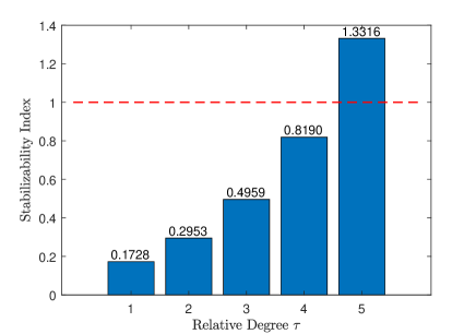
According to Theorem 2, the term on the left hand side of (69) indicates the mean-square input-output stabilizability of a networked feedback system. Once it is greater than one, no controller can stabilize the system in mean-square sense, i.e., the system is not mean-square input-output stabilizable. Here, we use this term as a mean-square stabilizability index for the system. For the plant with , namely , this mean-square stabilizability index is given by
which implies that the networked system can be stabilized by some controller in the mean-square sense. As shown by (69), the mean-square stabilizability index is also related to the relative degree of the plant . Since all the eigenvalues of are outside the unit disk, the mean-square stabilizability index in exponentially increases with respect to the relative degree. In this example, the stabilizability index with respect to the relative degree is shown in Fig. 5. When the relative degree grows to , the mean-square stabilizability index is greater than one and the system is not mean-square stabilizable.
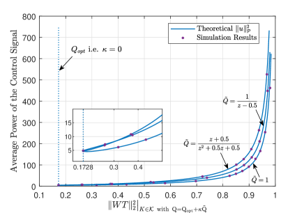
To verify Theorem 1, we also take in the plant (95) as an example. Since the mean-square input-output stability of the system means the boundedness of the average power of the control signal , it would be suitable to use the graph of against to visualize the stability or instability of the closed-loop system. Noticing that the networked system is mean-square input-output stabilizable, from Remark 8, a straightforward stabilizing controller of the networked system should be that in (57) with where is the solution to the equation (78). In this case, achieves its minimum, i.e., the stabilizability index, . Now let the controller be in of (57) with where and is a real nonnegative number. It turns out that, for a given , by varying from 0 to some sufficiently large number (dependent on ), would range from the stabilizability index to 1 such that the system is eventually unstable. For seeing this, three different ’s are taken into consideration, as shown in Fig. 6. By the Monte-Carlo method, the graphs of the theoretical and simulated average powers against associated with the ’s are also illustrated in Fig. 6, provided that the external input of the closed-loop system is a zero-mean Gaussian white noise with unit-variance. All average powers of the control signals would tend to infinity as approaches . This confirms Theorem 1 and implies that improper controller design would destabilize the closed-loop system.
6 Conclusion
In this paper, we have studied the mean-square input-output stability and stabilizability for a discrete-time LTI networked feedback system over an unreliable channel with random channel induced delays and packet dropout. Under a given linear receiving strategy, the models of the unreliable channel and related channel uncertainty are presented in time domain and frequency domain, respectively. In particular, frequency response of variation is introduced to describe the relative derivation of the unreliable channel. Applying these models, the mean-square input-output stability criterion is obtained for the networked feedback system. This is a general version of the mean-square small gain theorem for discrete-time LTI systems with i.i.d. stochastic multiplicative uncertainties. After then, the mean-square stabilizability is studied for the networked feedback system when its plant is minimum phase. A necessary and sufficient condition is found for the mean-square stabilizability of the networked feedback system via output feedback. This result shows the inherent connection between the mean-square stabilizability, the plant’s unstable poles and the frequency response of variation of the channel in the system.
It is straightforward to apply the proposed stability results to the so-called two-side networked control systems, i.e., systems with signal transmission via networks on both sensor and actuating channels. However, it can be shown that the stabilizability problem would become a decentralized control problem with information constraints, which precludes the convexity of the problem. Thus, exploring the stabilizability criteria for this type of systems will be focus of future research. It is also natural to consider the stability of the networked feedback system over the unreliable channel with deterministic constraints from the plant or/and the channel, which may turn out to be a mixed problem. Moreover, future work should include the stabilizability problems in a general setup of designable linear receiving strategy.
References
- [1] P. Antsaklis and J. Baillieul, “Special issue on technology of networked control systems,” Proceedings of the IEEE, vol. 95, pp. 5–8, Jan. 2007.
- [2] H. Sandberg, S. Amin, and K. H. Johansson, “Cyberphysical security in networked control systems: An introduction to the issue,” IEEE Control Systems Magazine, vol. 35, no. 1, pp. 20–23, 2015.
- [3] I. Jawhar, N. Mohamed, J. Al-Jaroodi, and S. Zhang, “An architecture for using autonomous underwater vehicles in wireless sensor networks for underwater pipeline monitoring,” IEEE Transactions on Industrial Informatics, vol. 15, no. 3, pp. 1329–1340, 2019.
- [4] A. Cuenca, D. J. Antunes, A. Castillo, P. García, B. A. Khashooei, and W. P. M. H. Heemels, “Periodic event-triggered sampling and dual-rate control for a wireless networked control system with applications to uavs,” IEEE Transactions on Industrial Electronics, vol. 66, no. 4, pp. 3157–3166, 2019.
- [5] H. Laaki, Y. Miche, and K. Tammi, “Prototyping a digital twin for real time remote control over mobile networks: Application of remote surgery,” IEEE Access, vol. 7, pp. 20325–20336, 2019.
- [6] E. J. Khatib, R. Barco, P. Munoz, I. De La Bandera, and I. Serrano, “Self-healing in mobile networks with big data,” IEEE Communications Magazine, vol. 54, no. 1, pp. 114–120, 2016.
- [7] J. P. Hespanha, P. Naghshtabrizi, and Y. Xu, “A survey of recent results in networked control systems,” Proceedings of the IEEE, vol. 95, pp. 138–162, Jan 2007.
- [8] P. Park, S. C. Ergen, C. Fischione, C. Lu, and K. H. Johansson, “Wireless network design for control systems: A survey,” IEEE Communications Surveys Tutorials, vol. 20, no. 2, pp. 978–1013, 2018.
- [9] D. Zhang, P. Shi, Q.-G. Wang, and L. Yu, “Analysis and synthesis of networked control systems: A survey of recent advances and challenges,” ISA Transactions, vol. 66, pp. 376 – 392, 2017.
- [10] M. S. Branicky, S. M. Phillips, and W. Zhang, “Stability of networked control systems: explicit analysis of delay,” in Proceedings of American Control Conference, vol. 4, pp. 2352–2357, June 2000.
- [11] G. C. Walsh, H. Ye, and L. Bushnell, “Stability analysis of networked control systems,” in Proceedings of American Control Conference, vol. 4, pp. 2876–2880, June 1999.
- [12] W. Zhang, M. S. Branicky, and S. M. Phillips, “Stability of networked control systems,” IEEE Control Systems, vol. 21, pp. 84–99, Feb 2001.
- [13] H. Lin and P. J. Antsaklis, “Stability and persistent disturbance attenuation properties for a class of networked control systems: switched system approach,” International Journal of Control, vol. 78, no. 18, pp. 1447–1458, 2005.
- [14] H. Lin and P. J. Antsaklis, “Stability and stabilizability of switched linear systems: A survey of recent results,” IEEE Transactions on Automatic Control, vol. 54, no. 2, pp. 308–322, 2009.
- [15] W.-A. Zhang and L. Yu, “Modelling and control of networked control systems with both network-induced delay and packet-dropout,” Automatica, vol. 44, no. 12, pp. 3206–3210, 2008.
- [16] X. Zhang, Q. Han, and X. Yu, “Survey on recent advances in networked control systems,” IEEE Transactions on Industrial Informatics, vol. 12, no. 5, pp. 1740–1752, 2016.
- [17] E. Fridman, U. Shaked, and V. Suplin, “Input/output delay approach to robust sampled-data control,” Systems and Control Letters, vol. 54, pp. 271–282, Mar. 2005.
- [18] V. Kharitonov and A. Zhabko, “Lyapunov-krasovskii approach to the robust stability analysis of time-delay systems,” Automatica, vol. 39, pp. 15–20, Jan. 2003.
- [19] V. L. Kharitonov and S. I. Niculescu, “On the stability of linear systems with uncertain delay,” IEEE Transactions on Automatic Control, vol. 48, pp. 127–132, Jan 2003.
- [20] J. Nilsson, B. Bernhardsson, and B. Wittenmark, “Stochastic analysis and control of real-time systems with random time delays,” Automatica, vol. 34, pp. 57–64, Jan. 1998.
- [21] J. Xiong and J. Lam, “Stabilization of networked control systems with a logic zoh,” IEEE Transactions on Automatic Control, vol. 54, pp. 358–363, Feb 2009.
- [22] M. Donkers, W. Heemels, D. Bernardini, A. Bemporad, and V. Shneer, “Stability analysis of stochastic networked control systems,” Automatica, vol. 48, no. 5, pp. 917 – 925, 2012.
- [23] D. Quevedo and J. Jurado, “Stability of sequence-based control with random delays and dropouts,” IEEE Transactions on Automatic Control, vol. 59, pp. 1296–1302, May 2014.
- [24] J. Xiong and J. Lam, “Stabilization of linear systems over networks with bounded packet loss,” Automatica, vol. 43, no. 1, pp. 80–87, 2007.
- [25] L. Zhang, Y. Shi, T. Chen, and B. Huang, “A new method for stabilization of networked control systems with random delays,” IEEE Transactions on Automatic Control, vol. 50, pp. 1177–1181, Aug 2005.
- [26] B. Chen, W. A. Zhang, and L. Yu, “Distributed fusion estimation with missing measurements, random transmission delays and packet dropouts,” IEEE Transactions on Automatic Control, vol. 59, pp. 1961–1967, July 2014.
- [27] L. Schenato, “Optimal estimation in networked control systems subject to random delay and packet drop,” IEEE Transactions on Automatic Control, vol. 53, pp. 1311–1317, June 2008.
- [28] L. Shi, M. Epstein, and R. M. Murray, “Kalman filtering over a packet-dropping network: A probabilistic perspective,” IEEE Transactions on Automatic Control, vol. 55, pp. 594–604, March 2010.
- [29] E. Ardestanizadeh and M. Franceschetti, “Control-theoretic approach to communication with feedback,” IEEE Transactions on Automatic Control, vol. 57, pp. 2576–2587, Oct 2012.
- [30] R. A. González, F. J. Vargas, and J. Chen, “Mean square stabilization over snr-constrained channels with colored and spatially correlated additive noises,” IEEE Transactions on Automatic Control, vol. 64, pp. 4825–4832, Nov 2019.
- [31] L. Schenato, “To zero or to hold control inputs with lossy links?,” IEEE Transactions on Automatic Control, vol. 54, no. 5, pp. 1093–1099, 2009.
- [32] N. Elia, “Remote stabilization over fading channels,” Systems & Control Letters, vol. 54, pp. 237–249, Mar. 2005.
- [33] N. Elia and J. N. Eisenbeis, “Limitations of linear control over packet drop networks,” IEEE Transactions on Automatic Control, vol. 56, pp. 826–841, April 2011.
- [34] T. Qi, J. Chen, W. Su, and M. Fu, “Control under stochastic multiplicative uncertainties: Part i, fundamental conditions of stabilizability,” IEEE Transactions on Automatic Control, vol. 62, pp. 1269–1284, March 2017.
- [35] W. J. Stewart, Probability, Markov Chains, Queues, and Simulation: The Mathematical Basis of Performance Modeling. USA: Princeton University Press, 2009.
- [36] G. Gu, “An equalization approach to feedback stabilization over fading channels,” IEEE Transactions on Automatic Control, vol. 61, pp. 1869–1881, July 2016.
- [37] W. Su, J. Chen, M. Fu, and T. Qi, “Control under stochastic multiplicative uncertainties: Part II, optimal design for performance,” IEEE Transactions on Automatic Control, vol. 62, pp. 1285–1300, March 2017.
- [38] B. A. Francis, A course in control theory. Springer-Verlag, 1987.
- [39] K. Zhou, J. C. Doyle, and K. Glover, Robust and Optimal Control. Pearson, 1995.
- [40] A. I. Maass and E. I. Silva, “Performance limits in the control of single-input linear time-invariant plants over fading channels,” IET Control Theory Applications, vol. 8, no. 14, pp. 1384–1395, 2014.