Mean Field Game GAN

Given a generator network $G_{\theta}$ and a discriminator network $D_{\omega}$, the original GAN objective is to find an mapping that maps a random noise to an expected distribution, it is written as a minimax problem

The loss function is derived from the cross-entropy between the real and generated distributions. Since we never know the ground truth distribution, when compared with other generative modeling approaches, GAN has lots of computational advantages. In GAN framework, it is easy to do sampling without requiring Markov chain, we utilize expectations which is also easy to compute to construct differentiable loss function. Finally, the framework naturally combine the advantages of neural networks, avoiding curse of dimensionality and is extended to various GANs with different objective functions. The disadvantage of original GAN is that the training process is delicate and unstable due to the reasons theoretically investigated in [2].

Wasserstein distance provides a better and more natural measure to evaluate the distance between two distributions[29]. The objective function of Wasserstein GAN is constructed on the basis of Kantorovich-Rubinstein duality form [28] for distributions $\rho_{1}$ and $\rho_{2}$

Given duality form, one would like to rewrite the duality form in a GAN framework by setting generator $G_{\theta}$, discriminator $D_{\omega}$ and then minimizing the Wasserstein distance between target distribution and generated distribution

Though WGAN has made a great success in various applications, it brings a well-known Lipschitz constraint problem, namely, we need to make our discriminator satisfies $\|\nabla D_{\omega}\leq 1\|$. Lipschitz constraint in WGAN has drawn a lot of attention of researchers, several methods such as weight clipping[3], adding gradient penalty as regularizer[13], applying weight normalization[27] and spectral normalization[24]. These methods enable convenience training process, however, besides these approximation-based method, we seek for a new formulation to avoid Lipschitz constraint in WGAN.

A variety of other GANs have been proposed in recent years. These GANs enlarge the application areas and provide great insights of designing generators and discriminators to facilitate the training process. One line of the work is focused on changing objective function such as f-GAN[25], Conditional-GAN[23], LS-GAN[22] and Cycle-GAN[30]. Another line is focused on developing stable structure of generator and discriminator, including DCGAN[26], Style-GAN[31] and Big-GAN[6]. Though these GANs has made a great success, there is no "best" GAN[20].

Hamilton-Jacobi equation in density space (HJD) plays an important role in optimal control problems[4, 7, 14]. HJD determines the global information of the system[10, 11] and describes the time evolution of the optimal value in density space. In applications, HJD has been shown very effective at modeling population differential games, also known as MFGs which study strategic dynamical interactions in large populations by extending finite players’ differential games[16, 12]. Within this context, the agents reach a Nash equilibrium at the optimum, where they can no longer unilaterally improve their objectives. The solutions to these problems are obtained by solving the following partial differential equations (PDEs)[9]

where $\rho(x,t)$ represents the population density of individual $x$ at time $t$. $\Phi(x,t)$ represents the velocity of population. We also have each player’s potential energy $f$ and terminal cost $g$. The Hamiltonian $H$ is defined as

where $L$ can be freely chosen.

Furthermore, a game is called a potential game when there exists a differentiable potential energy $F$ and terminal cost $G$, such that the MFG can be modeled as a optimal control problem in the density space[9]

where the infimum is taken among all vector fields $v(x,t)$ and densities $\rho(x,t)$ subject to the continuity equation

Our method is derived from this formulation, the details will be introduced in the next section.

To better understand the connections between MFGs and WGAN, we also would like to have a review on optimal transport(OT). OT rises as a popular topic in recent years, OT-based theories and formulations have been widely used in fluid mechanics[1], control[8], GANs[3] as well as PDE[21]. We study OT problem because it provides an optimal map $T$ to pushforward one probability distribution $\mu$ to another distribution $\nu$, with minimum cost $c$. One formulation is Monge’s optimal transport problem[28]

However, the solution of Monge problem may not exist and even if the solution exists, it may not be unique. Another formulation called Kantorovich’s optimal transport problem[5] reads

Notably, the fluid dynamic formulation of OT[5] reads

where $v(x,t)$ is the velocity vector. We solve this problem by applying Lagrange multiplier $\Phi(x,t)$ and optimality conditions, finally we have its dual form

We also refer readers to another related dynamical formulation of OT [17].

Let’s rewrite 6 and 7 with defining flux function $m(x,t)=\rho(x,t)v(x,t)$, then we have

with

We solve above primal-dual problem by applying Lagrange multiplier $\Phi(x,s)$

After integration by parts and reordering it leads to

where

Now let $L(x,v)=\frac{\|v\|^{p}}{p}$ where $\|\cdot\|$ can be any norm in Euclidean space. For example, choose $\|\cdot\|=\|\cdot\|_{2}$, namely, $\|v\|=\|v\|_{2}=\sqrt{v_{1}^{2}+v_{2}^{2}+...+v_{n}^{2}}$. For arbitrary norm $s$, we have the minimizer of 16 and corresponding $H$ as

Furthermore we have

Now we are able to plug $H(\nabla\Phi)$ back into 15, let $T=1$ and make $F$ and $G$ as 0, then

Next, we extend 21 to a GAN framework. We let $\rho(z,t)$ be the generator that pushforward Gaussian noise distribution to target distribution. Specially, we set $\rho_{1}$ as the distribution of our ground truth data. We treat $\Phi(x,t)$ as discriminator thus it leads to our objective function

We solve this minimax problem by algorithm 1. Notably, if we extend 22 to a general case with a general Hamiltonian $H$, we revise 22 as

Now we are going to derive the same objective function from the perspective of OT. Base on the formulation 11, we directly apply Lagrange multiplier $\rho(x,s)$ on the constraint to reformulate it as a saddle problem

We extend 24 to a GAN framework: we let $\rho(z,s)$ be the generator and $\Phi(x,s)$ as the discriminator thus finally we achieve the same problem

which has the same structure with 22, thus 22 can also be seen as minimizing Wasserstein-2 distance. A similar formulation is introduced in our recent work [19], where we consider two known distributions and compute their Wasserstein geodesic.

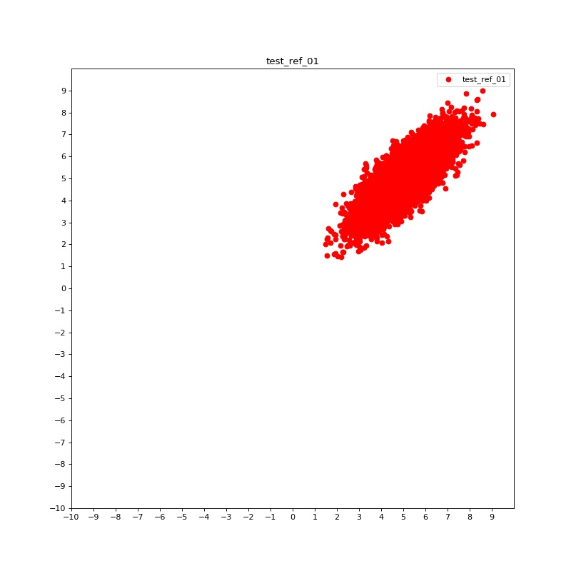
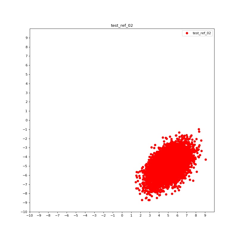
Syn-1: In this case we test our algorithm on 2D case, the target distribution is a Gaussian $\mathcal{N}(\mu,\Sigma)$, where $\mu$=(5,5) and $\Sigma$= [[1,0],[0,1]], here we choose $q=10,p=1.1$. The generated distributions are shown in Figure 1 (a) and (b).

Syn-2: Here and in all following tests we set $q=2,p=2$, in this case we still generate a 2D Gaussian distribution, with the same mean and covariance matrix we used in Syn-1. The generated distributions are shown in Figure 1 (c) and (d).

Syn-3: In this case we generate a 10D Gaussian as our target distribution. Some of 2D projections of the true distributions and generated distributions are shown in Figure 2.

MNIST: We first test our algorithm on MNIST data set. The generated handwritten digits are shown in Figure 3. We believe more carefully designed neural networks such as CNN with extra time input dimension will improve the quality of generated pictures.

References

- [1] M. Agueh, B. Khouider, and L.P. Saumier. Optimal transport for particle image velocimetry. In Communications in Mathematical Sciences, 2016.
- [2] M. Arjovsky and L. Bottou. Towards principled methods for training generative adversarial networks. arXiv: 1701.04862, 2017.
- [3] Martin Arjovsky, Soumith Chintala, and Léon Bottou. Wasserstein gan. In arXiv preprint arXiv:1701.07875, 2017.
- [4] J.D. Benamou and Y. Brenier. A computational fluid mechanics solution to the monge-kantorovich mass transfer problem. In Numerische Mathematik, 2000.
- [5] J.D. Benamou, B.D. Froese, and A.M. Oberman. Two numerical methods for the elliptic monge-ampere equation. ESAIM: Mathematical Modelling and Numerical Analysis, 44(4):737–758, 2010.
- [6] A. Brock, J. Donahue, and K. Simonyan. A style-based generator architecture for generative adversarial networks. In arXiv preprint arXiv:1809.11096, 2018.
- [7] P. Cardaliaguet, F. Delarue, J.M. Lasry, and P.L. Lions. The master equation and the convergence problem in mean field games. In arXiv preprint arXiv:1509.02505, 2015.
- [8] Y. Chen, T.T. Georgiou, and M. Pavon. On the relation between optimal transport and schrödinger bridges: A stochastic control viewpoint. In Journal of Optimization Theory and Applications, 2016.
- [9] Y.T. Chow, W. Li, S. Osher, and W. Yin. Algorithm for hamilton–jacobi equations in density space via a generalized hopf formula. Journal of Scientific Computing, 80(2):1195–1239, 2019.
- [10] W. Gangbo, T. Nguyen, and A. Tudorascu. Hamilton-jacobi equations in the wasserstein space. In Methods and Applications of Analysis, 2008.
- [11] W. Gangbo and A. Swiech. Existence of a solution to an equation arising from the theory of mean field games. In Journal of Differential Equations, 2015.
- [12] O. Gueant, J.M. Lasry, and P.L. Lions. Mean field games and applications. In In Paris-Princeton lectures on mathematical finance, 2010.
- [13] I. Gulrajani, F. Ahmed, M. Arjovsky, V. Dumoulin, and A.C. Courville. Improved training of wasserstein gans. In Advances in Neural Information Processing Systems, 2017.
- [14] M. Huang, R.P. Malhamé, and P.E. Caines. Large population stochastic dynamic games: closed-loop mckean-vlasov systems and the nash certainty equivalence principle. In Communications in Information & Systems, 2006.
- [15] Diederik P. Kingma and Jimmy Ba. Adam: A method for stochastic optimization, 2014.
- [16] J.M. Lasry and P.L. Lions. Mean field games. In Japanese journal of mathematics, 2007.
- [17] W. Li and S. Osher. Constrained dynamical optimal transport and its lagrangian formulation. In arXiv preprint arXiv:1807.00937, 2018.
- [18] A.T. Lin, S.W. Fung, W. Li, L. Nurbekyan, and S.J. Osher. Apac-net: Alternating the population and agent control via two neural networks to solve high-dimensional stochastic mean field games. In arXiv preprint arXiv:2002.10113, 2020.
- [19] S. Liu, S. Ma, Y. Chen, H. Zha, and H. Zhou. Learning high dimensional wasserstein geodesics. In arXiv preprint arXiv:2102.02992, 2021.
- [20] M. Lucic, K. Kurach, M. Michalski, S. Gelly, and O. Bousquet. Are gans created equal? a large-scale study. In Advances in Neural Information Processing Systems, 2018.
- [21] S. Ma, S. Liu, H. Zha, and H. Zhou. Learning stochastic behaviour of aggregate data. In arXiv preprint arXiv:2002.03513, 2020.
- [22] X. Mao, Q. Li, H. Xie, Lau R.Y., Wang Z., and S. Paul Smolley. Least squares generative adversarial networks. In International Conference on Computer Vision, 2017.
- [23] M. Mirza and S. Osindero. Conditional generative adversarial nets. In arXiv preprint arXiv:1411.1784, 2014.
- [24] T. Miyato, T. Kataoka, M. Koyama, and Y. Yoshida. Spectral normalization for generative adversarial networks. In arXiv preprint arXiv:1802.05957, 2018.
- [25] S. Nowozin, B. Cseke, and R. Tomioka. f-gan: Training generative neural samplers using variational divergence minimization. In Advances in Neural Information Processing Systems, pages 271–279, 2016.
- [26] A. Radford, L. Metz, and S. Chintala. Unsupervised representation learning with deep convolutional generative adversarial networks. In arXiv preprint arXiv:1511.06434, 2015.
- [27] T. Salimans and D.P. Kingma. Weight normalization: A simple reparameterization to accelerate training of deep neural networks. In Advances in Neural Information Processing Systems, 2016.
- [28] C. Villani. Optimal transport: old and new, volume 338. Springer Science & Business Media, 2008.
- [29] Cédric Villani. Topics in optimal transportation. Number 58. American Mathematical Soc., 2003.
- [30] J.Y. Zhu, T. Park, P. Isola, and A.A. Efros. Unpaired image-to-image translation using cycle-consistent adversarial networks. In International Conference on Computer Vision, 2017.
- [31] T. ZKarras, S. Laine, and T. Aila. A style-based generator architecture for generative adversarial networks. In International Conference on Computer Vision and Pattern Recognition, 2019.