\addauthor

rrred \addauthorjwbrown \addauthorarred \addauthorbcblue \addauthordmtblue

Mean Estimation in Banach Spaces
Under Infinite Variance and Martingale Dependence

Justin Whitehouse Computer Science Department, Carnegie Mellon University Ben Chugg Machine Learning Department, Carnegie Mellon University Department of Statistics and Data Science, Carnegie Mellon University^†^†thanks: {jwhiteho,diegomar}@andrew.cmu.edu, {benchugg,aramdas}@cmu.edu
Diego Martinez-Taboada Department of Statistics and Data Science, Carnegie Mellon University^†^†thanks: {jwhiteho,diegomar}@andrew.cmu.edu, {benchugg,aramdas}@cmu.edu Aaditya Ramdas Machine Learning Department, Carnegie Mellon University Department of Statistics and Data Science, Carnegie Mellon University^†^†thanks: {jwhiteho,diegomar}@andrew.cmu.edu, {benchugg,aramdas}@cmu.edu

Abstract

We consider estimating the shared mean of a sequence of heavy-tailed random variables taking values in a Banach space. In particular, we revisit and extend a simple truncation-based mean estimator by Catoni and Giulini. While existing truncation-based approaches require a bound on the raw (non-central) second moment of observations, our results hold under a bound on either the central or non-central $p$ th moment for some $p>1$ . In particular, our results hold for distributions with infinite variance. The main contributions of the paper follow from exploiting connections between truncation-based mean estimation and the concentration of martingales in 2-smooth Banach spaces. We prove two types of time-uniform bounds on the distance between the estimator and unknown mean: line-crossing inequalities, which can be optimized for a fixed sample size $n$ , and non-asymptotic law of the iterated logarithm type inequalities, which match the tightness of line-crossing inequalities at all points in time up to a doubly logarithmic factor in $n$ . Our results do not depend on the dimension of the Banach space, hold under martingale dependence, and all constants in the inequalities are known and small.

1 Introduction

Mean estimation is perhaps the most important primitive in the statistician’s toolkit. When the data is light-tailed (perhaps sub-Gaussian, sub-Exponential, or sub-Gamma), the sample mean is the natural estimator of this unknown population mean. However, when the data fails to have finite moments, the naive plug-in mean estimate is known to be sub-optimal.

The failure of the plug-in mean has led to a rich literature focused on heavy-tailed mean estimation. In the univariate setting, statistics such as the thresholded/truncated mean estimator [40, 21], trimmed mean estimator [35, 29], median-of-means estimator [34, 22, 2], and the Catoni M-estimator [5, 42] have all been shown to exhibit favorable convergence guarantees. When a bound on the variance of the observations is known, many of these estimates enjoy sub-Gaussian rates of performance [26], and this rate gracefully decays when only a bound on the $p$ th central moment is known for some $p>1$ [3].

In the more challenging setting of multivariate heavy-tailed data, modern methods include the geometric median-of-means estimator [33], the median-of-means tournament estimator [28], and the truncated mean estimator [6]. We provide a more detailed account in Section 1.2.

Of the aforementioned statistics, the truncated mean estimator is by far the simplest. This estimator, which involves truncating observations to lie within an appropriately-chosen ball centered at the origin, is extremely computationally efficient and can be updated online, very desirable for applied statistical tasks. However, this estimator also possesses a number of undesirable properties. First, it is not translation invariant, with bounds that depend on the raw moments of the random variables. Second, it requires a known bound on the $p$ th moment of observations for some $p\geq 2$ , thus requiring that the observations have finite variance. Third, bounds are only known in the setting of finite-dimensional Euclidean spaces — convergence is not understood in the setting of infinite-dimensional Hilbert spaces or Banach spaces.

The question we consider here is simple: are the aforementioned deficiencies fundamental to truncation-based estimators, or can they be resolved with an improved analysis? The goal of this work is to show that the latter is true, demonstrating how a truncation-based estimator can be extended to handle fewer than two central moments in general classes of Banach spaces.

1.1 Our Contributions

In this work, we revisit and extend a simple truncation-based mean estimator due to Catoni and Giulini [6]. Our estimator works by first using a small number of samples to produce a naive mean estimate, say through a sample mean. Then, the remaining sequence of observations is truncated to lie in an appropriately-sized ball centered at this initial mean estimate. These truncated samples are then averaged to provide a more robust estimate of a heavy-tailed mean.

While existing works study truncation-based estimators via PAC-Bayesian analyses [6, 11, 24], we find it more fruitful to study these estimators using tools from the theory of Banach space-valued martingales. In particular, by proving a novel extension of classical results on the time-uniform concentration of bounded martingales due to Pinelis [36, 37], we are able to greatly improve the applicability of truncation-based estimators. In particular, our estimator and analysis improves over that in [6] in the following ways:

1.

The analysis holds in arbitrary 2-smooth Banach spaces instead of just finite-dimensional Euclidean space. This not only includes Hilbert spaces but also the commonly-studied $L^{\alpha}$ and $\ell^{\alpha}$ spaces for $2\leq\alpha<\infty$ .
2.

Our results require only a known upper bound on the conditional central $p$ th moment of observations for some $p>1$ , and are therefore applicable to data lacking finite variance. Existing bounds for truncation estimators, on the other hand, require a bound on the non-central second moment.
3.

Our bounds are time-uniform and hold for data with a martingale dependence structure. We prove two types of inequalities: line-crossing inequalities, which can be optimized for a target sample size, and non-asymptotic law of the iterated logarithm (LIL) type inequalities, which match the tightness of the boundary-crossing inequalities at all times simultaneously up to a doubly logarithmic factor in the sample size.
4.

We show that our estimator exhibits strong practical performance, and that our derived bounds are tighter than existing results in terms of constants. We run simulations which demonstrate that, for appropriate truncation diameters, the distance between our estimator and the unknown mean is tightly concentrated around zero.

Informally, if we assume that the central $p$ th moments of all observations are conditionally bounded by $v$ , and we let $\widehat{\mu}_{n}$ denote our estimate after $n$ samples, then we show that

\|\widehat{\mu}_{n}-\mu\|=O\left(v^{1/p}(\log(1/\delta)/n)^{\frac{p-1}{p}}\right)\qquad\text{with probability }\geq 1-\delta.

As far as we are aware, the only other estimator to obtain the same guarantee in a similar setting is Minsker’s geometric median-of-means [33]. (While he doesn’t state this result explicitly, it is easily derivable from his main bound—see Appendix B for the details.) Minsker also works in a Banach space, but assumes that it is separable and reflexive, whereas we will assume that it is separable and smooth. While we obtain the same rates, we feel that our truncation-style estimator has several benefits over geometric median-of-means. First, it is computationally lightweight and easy to compute exactly. Second, our line-crossing inequalities do not require as many tuning parameters to instantiate (eg choice of $\alpha^{*}$ , $\gamma^{*}$ , or $B$ ; see Section B). Third, we handle martingale dependence while Minsker does not. Finally, our analysis is significantly different from Minsker’s—and from existing analyses of other estimators under heavy-tails—and may be of independent interest.

1.2 Related Work

Section 1.1 discussed the relationship between this paper and the two most closely related works of Catoni and Giulini [6] and Minsker [33]. We now discuss how our work is related to the broader literature, none of which addresses our problem directly, but tackles simpler special cases of our problem (e.g., assuming more moments or boundedness, or with observations in Hilbert spaces or Euclidean spaces).

Heavy-tailed mean estimation under independent observations.

Truncation-based (also called threshold-based) estimators have a rich history in the robust statistics literature, dating back to works from Tukey, Huber, and others [21, 40]. These estimators have either been applied in the univariate setting or in $\mathbb{R}^{d}$ as in Catoni and Giulini [6]. A related estimator is the so-called trimmed-mean estimator, which removes extreme observations and takes the empirical mean of the remaining points [35, 29]. For real-valued observations with finite variance, the trimmed-mean has sub-Gaussian performance [35].

Separately, Catoni and Giulini [5] introduce an approach for mean estimation in $\mathbb{R}^{d}$ based on M-estimators with a family of appropriate influence functions. This has come to be called “Catoni’s M-estimator.” It requires at least two moments and fails to obtain sub-Gaussian rates. It faces the the additional burden of being less computationally efficient. A series of followup works have improved this estimator in various ways: Chen et al. [7] extend it to handle a $p$ -th moment for $p\in(1,2)$ for real-valued observations, Gupta et al. [15] refine and sharpen the constants, and Mathieu [32] studies the optimality of general M-estimators for mean estimation.

Another important line of work on heavy-tailed mean estimation is based on median-of-means estimators [34, 22, 2]. These estimators generally break a dataset into several folds, compute a mean estimate on each fold, and then compute some measure of central tendency amongst these estimates. For real-valued observations, Bubeck et al. [3] study a median-of-means estimator that holds under infinite variance. Their estimator obtains the same rate as ours and Minsker’s. Most relevant for our work is the result on geometric median-of-means due to Minsker [33], which can be used to aggregate several independent mean estimates in general separable Banach spaces. In Hilbert spaces, when instantiated with the empirical mean under a finite variance assumption, geometric median-of-means is nearly sub-Gaussian (see discussion in Section 1.1). We compare our threshold-based estimator extensively to geometric median-of-means in the sequel and demonstrate that we obtain the same rate of convergence.

Another important result is the multivariate tournament median-of-means estimator due to Lugosi and Mendelson [28]. For i.i.d. observations in $(\mathbb{R}^{d},\|\cdot\|_{2})$ with shared covariance matrix (operator) $\Sigma$ , then Lugosi and Mendelson [28] show this estimator can obtain the optimal sub-Gaussian rate of $O(\sqrt{\Tr(\Sigma)/n}+\sqrt{\|\Sigma\|_{\text{op}}\log(1/\delta)/n})$ . However, this result requires the existence of a covariance matrix and does not extend to a bound on the $p$ -th moment for $p\in(1,2)$ , which is the main focus of this work.

While the original form of the tournament median-of-means estimator was computationally inefficient (with computation hypothesized to be NP-Hard in a survey by Lugosi and Mendelson [26]), a computationally efficient approximation was developed by Hopkins [17], with followup work improving the running time [8]. Tournament median-of-means was extended to general norms in $\mathbb{R}^{d}$ [27], though the authors note that this approach is still not computationally feasible. Median-of-means style approaches have also been extended to general metric spaces [20, 9]. Of the above methods, only the geometric median-of-means estimator can handle observations that lack finite variance.

Sequential concentration under martingale dependence.

Time-uniform concentration bounds, or concentration inequalities that are valid at data-dependent stopping times, have been the focus of significant recent attention [18, 19, 44]. Such results are often obtained by identifying an underlying nonnegative supermartingale and then applying Ville’s inequality [41], a strategy that allows for martingale dependence quite naturally. This approach is also used here. Wang and Ramdas [42] extend Catoni’s M-estimator to handle both infinite variance and martingale dependence in $\mathbb{R}$ , while Chugg et al. [11] give a sequential version of the truncation estimator in $\mathbb{R}^{d}$ , though they require a central moment assumption and finite variance. The analyses of both Catoni and Giulini [6] and Chugg et al. [11] rely on so-called “PAC-Bayes” arguments [4, 12]. Intriguingly, while we analyze a similar estimator, our analysis avoids such techniques and is much closer in spirit to Pinelis-style arguments [36, 37].

Howard et al. [18, 19] provide a general collection of results on time-uniform concentration for scalar processes, which in particular imply time-uniform concentration results for some heavy-tailed settings (e.g. symmetric observations). Likewise, Whitehouse et al. [44] provide a similar set of results in $\mathbb{R}^{d}$ . While interesting, we note that these results differ from our own in that they are self-normalized, or control the growth of a process appropriately normalized by some variance proxy (here a mixture of adapted and predictable covariance). The results also don’t apply when only a bound on the $p$ th moment is known, and the latter set of results have explicit dependence on the ambient dimension $d$ .

Concentration in Hilbert and Banach Spaces.

There are several results related to concentration in infinite-dimensional spaces. A series of works has developed self-normalized, sub-Gaussian concentration bounds in Hilbert spaces [43, 1, 10] based on the famed method of mixtures [13, 14]. These results have not been extended to more general tail conditions. Significant progress has been made on the concentration of bounded random variables in smooth and separable Banach spaces. Pinelis [36, 37] presented a martingale construction for bounded observations, thus enabling dimension-free Hoeffding and Bernstein inequalities. Dimension-dependence is replaced by the smoothness parameter of the Banach space, which for most practical applications (in Hilbert spaces, say) equals one. These results were strengthened slightly by Howard et al. [18]. Recently, Martinez-Taboada and Ramdas [31] gave an empirical-Bernstein inequality in Banach spaces, also using a Pinelis-like construction. Our work adds to this growing literature by extending Pinelis’ tools to the heavy-tailed setting.

1.3 Preliminaries

We introduce some of the background and notation required to state our results. We are interested in estimating the shared, conditional mean $\mu$ of a sequence of random variables $(X_{n})_{n\geq 1}$ living in some separable Banach space $(\mathbb{B},\|\cdot\|)$ . Recall that a Banach space is a complete normed vector space; examples include Hilbert spaces, $\ell^{\alpha}$ sequence spaces, and $L^{\alpha}$ spaces of functions. We make the following central assumption.

Assumption 1.

We assume $(X_{n})_{n\geq 1}$ are a sequence of $\mathbb{B}$ -valued random variables adapted to a filtration $\mathcal{F}\equiv(\mathcal{F}_{n})_{n\geq 0}$ such that

(1)

$\mathbb{E}(X_{n}\mid\mathcal{F}_{n-1})=\mu$ , for all $n\geq 1$ and some unknown $\mu\in\mathbb{B}$ , and
(2)

$\sup_{n\geq 1}\mathbb{E}\left(\|X_{n}-\mu\|^{p}\mid\mathcal{F}_{n-1}\right)\leq v<\infty$ for some known constants $p\in(1,2]$ and $v>0$ .

The martingale dependence in condition (1) above is weaker than the traditional i.i.d. assumption, requiring only a constant conditional mean. This is useful in applications such as multi-armed bandits, where we cannot assume that the next observation is independent of the past. Meanwhile, condition (2) allows for infinite variance, a weaker moment assumption than past works studying concentration of measure in Banach spaces (e.g., [33, 36, 37]). In Appendix C we replace condition (2) with a bound on the raw moment (that is, $\mathbb{E}(\|X_{n}\|^{p}|\mathcal{F}_{n-1})$ ) for easier comparison with previous work. We note that other works studying truncation-based estimators have exclusively considered the $p\geq 2$ setting where observations admit covariance matrices [11, 6, 26]. We focus on $p\in(1,2]$ in this work, but it is likely our techniques could be naturally extended to the $p\geq 2$ setting. We leave this as interesting future work.

In order obtain concentration bounds, we must assume the Banach space is reasonably well-behaved. This involves assuming that is it both separable and smooth. A space is separable if it contains a countable, dense subset, and a real-valued function $f:\mathbb{B}\to\mathbb{R}$ is $(2,\beta)$ -smooth if, for all $x,y\in\mathbb{B}$ , $f(0)=0$ , $|f(x+y)-f(x)|\leq\|y\|$ , and

f^{2}(x+y)+f^{2}(x-y)\leq 2f^{2}(x)+2\beta^{2}\|y\|^{2}.

(1.1)

We assume that the norm is smooth in the above sense.

Assumption 2.

We assume that the Banach space $(\mathbb{B},\|\cdot\|)$ is both separable and $(2,\beta)$ -smooth, meaning that the norm satisfies (1.1).

Assumption 2 is common when studying Banach spaces [36, 37, 18, 31]. We emphasize that $\beta$ is not akin to the dimension of the space. For instance, infinite-dimensional Hilbert spaces have $\beta=1$ and $L^{\alpha}$ and $\ell^{\alpha}$ spaces have $\beta=\sqrt{\alpha-1}$ for $\alpha\geq 2$ . Thus, bounds which depend on $\beta$ are still dimension-free.

Notation and background.

For notational simplicity, we define the conditional expectation operator $\mathbb{E}_{n-1}[\cdot]$ to be $\mathbb{E}_{n-1}[X]:=\mathbb{E}(X\mid\mathcal{F}_{n-1})$ for any $n\geq 1$ . If $S\equiv(S_{n})_{n\geq 0}$ is some stochastic process, we denote the $n$ -th increment as $\Delta S_{n}:=S_{n}-S_{n-1}$ for any $n\geq 1$ . For any process or sequence $a\equiv(a_{n})_{n\geq 1}$ , denote by $a^{n}$ the first $n$ values: $a^{n}=(a_{1},\dots,a_{n})$ . We say the process $S$ is predictable with respect to filtration $\mathcal{F}$ , if $S_{n}$ is $\mathcal{F}_{n-1}$ -measurable for all $n\geq 1$ . Our analysis will make use of both the Fréchet and Gateaux derivatives of functions in a Banach space. We do not define these notions here but instead refer to Ledoux and Talagrand [25].

Outline.

Section 2 provides statements of the main results. Our main result, Theorem 2.1, is a general template for obtaining bounds (time-uniform boundary-crossing inequalities in particular) on truncation-style estimators. Corollary 2.2 then instantiates the template with particular parameters to obtain tightness for a fixed sample size. Section 3 is dedicated to the proof of Theorem 2.1. Section 4 then uses a technique known as “stitching” to extend our line-crossing inequalities to bounds which shrink to zero over time at an iterated logarithm rate. Finally, Section 5 provides several numerical experiments demonstrating the efficacy of our proposed estimator in practice.

2 Main Result

Define the mapping

\mathtt{Trunc}:\mathbb{B}\rightarrow[0,1]\text{\leavevmode\nobreak\ by \leavevmode\nobreak\ }x\mapsto\frac{1\land\|x\|}{\|x\|}.

(2.1)

Clearly, $\mathtt{Trunc}(x)x$ is just the projection of $x$ onto the unit ball in $B$ . Likewise, $\mathtt{Trunc}(\lambda x)x$ is the projection of $x$ onto the ball of radius $\lambda^{-1}$ in $B$ . We note that the truncated observations $\mathtt{Trunc}(X_{n})X_{n}$ are themselves random variables, which are adapted to the underlying filtration $\mathcal{F}$ .

As we discussed in Section 1.1, previous analyses of truncation-style estimators have relied on a bound on the raw second moment. To handle a central moment assumption, we will center our estimator around a naive mean estimate which has worse guarantees but whose effects wash out over time.

To formalize the above, our estimate of $\mu$ at time $n$ will be

\widehat{\mu}_{n}(k)\equiv\widehat{\mu}_{n}(k,\lambda,\widehat{Z}_{k}):=\frac{1}{n}\sum_{k<m\leq n}\big{\{}\mathtt{Trunc}(\lambda(X_{m}-\widehat{Z}_{k}))(X_{m}-\widehat{Z}_{k})+\widehat{Z}_{k}\big{\}},

(2.2)

where $\widehat{Z}_{k}$ is a naive mean estimate formed using the first $k$ samples and $\lambda>0$ is some fixed hyperparameter. Defining $\widehat{Z}_{0}=0$ when $k=0$ , we observe that $\widehat{\mu}_{n}(0)$ is the usual truncation estimator, analyzed by Catoni and Giulini [6] in the fixed-time setting and Chugg et al. [11] in the sequential setting. To state our result, define

K_{p}:=\frac{1}{p/q+1}\left(\frac{p/q}{p/q+1}\right)^{p/q}\text{\leavevmode\nobreak\ where \leavevmode\nobreak\ }\frac{1}{p}+\frac{1}{q}=1,

(2.3)

which depends on the Holder conjugate $q$ of $p$ . Note that $K_{p}<1$ for all $p>1$ . In fact, $\lim_{p\to 1}K_{p}=1$ , $\lim_{p\to\infty}K_{p}=0$ , and $K_{p}$ is decreasing in $p$ . We also define the constant

\mathfrak{C}_{p}(\mathbb{B})=\begin{cases}2^{p-1}(\frac{e^{2}-3}{4}),&\text{if }(\mathbb{B},\|\cdot\|)\text{ is a Hilbert space},\\ \beta^{2}2^{p+1}(\frac{e^{2}-3}{4}),&\text{otherwise},\end{cases}

(2.4)

which depends on the geometry and smoothness $\beta$ of the Banach space $(\mathbb{B},\|\cdot\|)$ . In a Hilbert space (for which $\beta=1$ ), the variance of our supermartingale increments can be more easily bounded. If the norm is not induced by an inner product, then $\mathfrak{C}_{p}(\mathbb{B})$ suffers an extra factor of four. Note that $\frac{e^{2}-3}{4}<1.1$ .

Our main result is the following template for bounding the deviations of $\widehat{\mu}_{n}$ assuming some sort of concentration of $\widehat{Z}_{k}$ around $\mu$ .

Theorem 2.1 (Main result).

Let $X_{1},X_{2},\dots$ be random variables satisfying Assumption 1 which lie in some Banach space $(\mathbb{B},\|\cdot\|)$ satisfying Assumption 2. Suppose we use the first $k$ samples to construct $\widehat{Z}_{k}$ which satisfies, for any $\delta\in(0,1]$ ,

\mathbb{P}(\|\mu-\widehat{Z}_{k}\|\geq r(\delta,k))\leq\delta,

(2.5)

for some function $r:(0,1]\times\mathbb{N}\to\mathbb{R}_{\geq 0}$ . Fix any $\delta\in(0,1]$ . Decompose $\delta$ as $\delta=\delta_{1}+\delta_{2}$ where $\delta_{1},\delta_{2}>0$ . Then, for any $\lambda>0$ , with probability $1-\delta$ , simultaneously for all $n\geq k$ , we have:

\left\|\widehat{\mu}_{n}(k,\lambda,\widehat{Z}_{k})-\mu\right\|\leq\lambda^{p-1}(\mathfrak{C}_{p}(\mathbb{B})+K_{p}2^{p-1})(v+r(\delta_{2},k)^{p})+\frac{\log(2/\delta_{1})}{\lambda(n-k)}.

(2.6)

The guarantee provided by Theorem 2.1 is a line-crossing inequality in the spirit of [18]. That is, if we multiply both sides by $n-k$ , it provides a time-uniform guarantee on the probability that the left hand side deviation between $\widehat{\mu}_{n}$ and $\mu$ ever crosses the line parameterized by the right hand side of (2.6). If we optimize the value of $\lambda$ for a particular sample size $n^{*}$ , the bound will remain valid for all sample sizes, but will be tightest at and around $n=n^{*}$ . To obtain bounds that are tight for all $n$ simultaneously, one must pay an additional iterated logarithmic price in $n$ . To accomplish this, Section 4 will deploy a carefully designed union bound over geometric epochs—a technique known as “stitching” [19]. However, for practical applications where the sample size is known in advance, we recommend Theorem 2.1 and its corollaries.

Next we provide a guideline on choosing $\lambda$ in Theorem 2.1. The proof is straightforward but is provided in Appendix A for completeness.

Corollary 2.2.

In Theorem 2.1, consider taking

\lambda=\left(\frac{\log(2/\delta_{1})}{(\mathfrak{C}_{p}(\mathbb{B})+K_{p}2^{p-1})(n-k)(v+r(\delta_{2},k)^{p})}\right)^{1/p}.

(2.7)

Then, with probability at least $1-\delta_{1}-\delta_{2}$ , we have

\|\widehat{\mu}_{n}(k)-\mu\|\leq\Big{(}(\mathfrak{C}_{p}(\mathbb{B})+K_{p}2^{p-1})(v+r(\delta_{2},k)^{p})\Big{)}^{1/p}\left(\frac{\log(2/\delta_{1})}{n-k}\right)^{(p-1)/p}.

In particular, as long as $k=o(n)$ , $r(\delta,k)=o(1)$ and $\delta_{1},\delta_{2}=\Theta(\delta)$ , we have

\|\widehat{\mu}_{n}(k)-\mu\|=O\left(v^{1/p}\left(\frac{\log(1/\delta)}{n}\right)^{(p-1)/p}\right).

(2.8)

This is the desired rate per the discussion in Section 1.1, matching the rate of other estimators which hold under infinite variance. In particular, it matches the rates of Bubeck et al. [3] in scalar settings and Minsker [33] in Banach spaces.

Now let us instantiate Theorem 2.1 when we take $\widehat{Z}_{k}$ to be either the sample mean or Minsker’s geometric median-of-means. The latter provides a better dependence on $\delta_{2}$ but at an additional computational cost. As we’ll see in Section 5, this benefit is apparent for small sample sizes, but washes out as $n$ grows. The details of the proof can be found in Appendix A.

Corollary 2.3.

Let $(\mathbb{B},\|\cdot\|)$ satisfy Assumption 2 and $X_{1},\dots,X_{n}$ satisfy Assumption 1. For some $k<n$ , let $\widehat{Z}_{k}$ be the empirical mean of the first $k$ observations. Given $\delta>0$ , decompose it as $\delta=\delta_{1}+\delta_{2}$ for any $\delta_{1},\delta_{2}>0$ . Then, with probability $1-\delta$ ,

\|\widehat{\mu}_{n}(k)-\mu\|\leq 2v^{1/p}C_{p}^{1/p}\left(\frac{\log(2/\delta_{1})}{(n-k)^{1/p}}\right)^{(p-1)/p}\left(1+O\left(\frac{1}{\delta_{2}k^{p-1}}\right)\right),

(2.9)

where $C_{p}=\mathfrak{C}_{p}(\mathbb{B})+K_{p}2^{p-1}$ . If, on the other hand, $\widehat{Z}_{k}$ is the geometric median-of-means estimator with appropriate tuning parameters, then with probability $1-\delta$ ,

\|\widehat{\mu}_{n}(k)-\mu\|\leq 2v^{1/p}C_{p}^{1/p}\left(\frac{\log(2/\delta_{1})}{(n-k)^{1/p}}\right)^{1-1/p}\left(1+O\left(\frac{\log(1/\delta_{2})^{(p-1)/p}}{k^{(p-1)/p}}\right)\right).

(2.10)

When $\widehat{Z}_{k}$ is the empirical mean, if $k=k(n)=\lfloor\log_{2}(n)\rfloor$ (say), we have $n-k(n)\geq n/2$ for $n\geq 2$ , so (2.9) recovers the rate in (2.8), since the additional factor of $O(\frac{1}{\delta_{2}k(n)^{p-1}})=O(\frac{1}{\delta_{2}\log(n)^{p-1}})$ is $o(1)$ and vanishes. When $\widehat{Z}_{k}$ is the geometric median-of-means, this error term vanishes even faster.

3 Proof of Theorem 2.1

We will prove a slightly more general result that reduces to Theorem 2.1 in a special case. Throughout this section, fix two $\mathcal{F}$ -predictable sequences, $(\widehat{Z}_{n})\in\mathbb{B}^{\mathbb{N}}$ and $(\lambda_{n})\in\mathbb{R}_{+}^{\mathbb{N}}$ . Define

\widehat{\xi}_{n}\equiv\widehat{\xi}_{n}(\lambda^{n},Z^{n}):=\sum_{m\leq n}\lambda_{m}\big{\{}\mathtt{Trunc}(\lambda_{m}Y_{m})Y_{m}+\widehat{Z}_{m}\big{\}}\text{\leavevmode\nobreak\ where \leavevmode\nobreak\ }Y_{m}:=X_{m}-\widehat{Z}_{m},

(3.1)

If we take $\lambda_{n}$ to be constant and $\widehat{Z}_{m}=\widehat{Z}$ to be $\mathcal{F}_{0}$ -measurable, then $\widehat{\xi}_{n}=n\lambda\widehat{\mu}_{n}$ . We will make such a substitution at the end of this analysis to prove the desired result. However, working with the more general process (2.2) has advantages. In particular, it allows us to consider sequences of predictable mean-estimates, if desired.

Our preliminary goal is to find a process $(V_{n})_{n\geq 0}$ such that the process

M_{n}(\lambda^{n})=\exp\left\{\bigg{\|}\widehat{\xi}_{n}-\mu\sum_{m\leq n}\lambda_{m}\bigg{\|}-V_{n}(\lambda^{n})\right\},

(3.2)

is upper bounded by a nonnegative supermartingale; in other words; in recent parlance, it is an e-process [38]. Applying Ville’s inequality will then give us a time-uniform bound on the deviation of the process $\|(\sum_{m\leq n}\lambda_{m})^{-1}\widehat{\xi}_{n}-\mu\|$ in terms of $V_{n}(\lambda)$ . We will let

		$\displaystyle V_{n}(\lambda)=(\mathfrak{C}_{p}(\mathbb{B})+K_{p}2^{p-1})G_{n},$
	where	$\displaystyle G_{n}\equiv G_{n}(\lambda^{n},\widehat{Z}^{n}):=\sum_{m\leq n}\lambda_{m}^{p}(v+\\|\mu-\widehat{Z}_{m}\\|^{p}),$		(3.3)

is a weighted measure of the deviation of the naive estimates $\widehat{Z}_{1},\dots,\widehat{Z}_{n}$ from $\mu$ . Since it is difficult to reason about the difference between $\widehat{\xi}_{n}$ and $\mu\sum_{m\leq n}\lambda_{m}$ directly, we introduce the proxy

\widetilde{\mu}_{n}(\lambda):=\mathbb{E}_{n-1}[\mathtt{Trunc}(\lambda Y_{n})Y_{n}]+\widehat{Z}_{n},

(3.4)

and argue about $\|\widehat{\xi}_{n}-\sum_{m\leq n}\lambda_{m}\widetilde{\mu}_{m}(\lambda_{m})\|$ and $\lambda_{m}\|\widetilde{\mu}_{m}(\lambda_{m})-\mu\|$ . We then bound the difference $\|\widehat{\xi}_{n}-\mu\sum_{m\leq n}\lambda_{m}\|$ using the triangle inequality.

3.1 Step 1: Bounding $\|\widetilde{\mu}_{n}(\lambda)-\mu\|$

We need the following analytical property of $\mathtt{Trunc}$ , which will be useful in bounding the truncation error with fewer than two moments. We note that the following lemma was used by Catoni and Giulini [6] for $k\geq 1$ . We prove the result for $k>0$ .

Lemma 3.1.

For any $k>0$ and $x\in\mathbb{B}$ , we have that

1-\mathtt{Trunc}(x)\leq\frac{\|x\|^{k}}{k+1}\left(\frac{k}{k+1}\right)^{k}.

Proof.

Fix $k>0$ . It suffices to show that $f(t):=1-\frac{1\land t}{t}\leq\frac{t}{k+1}\left(\frac{k}{k+1}\right)^{k}=:g_{k}(t)$ for all $t\geq 0$ . For $t\in[0,1],$ the result is obvious. For $t\geq 1$ , we need to do a bit of work. First, note that $g_{k}(1)>f(1)=0$ , and that both $g_{k}$ and $f$ are continuous. Further, we only have $g_{k}(t)=f(t)$ precisely when $t=\frac{k+1}{k}$ . Let this value of $t$ be $t^{\ast}$ . This immediately implies that $g_{k}(t)\geq f(t)$ for $t\in[1,t^{\ast}]$ . To check the inequality for all $t\geq t^{\ast}$ , it suffices to check that $f^{\prime}(t)<g_{k}^{\prime}(t)$ . We verify this by direct computation. First, $f^{\prime}(t)=\frac{1}{t^{2}}$ . Likewise, we have that $g_{k}^{\prime}(t)=t^{k-1}\left(\frac{k}{k+1}\right)^{k+1}$ . Taking ratios, we see that

\frac{g_{k}^{\prime}(t)}{f^{\prime}(t)}=t^{k+1}\left(\frac{k}{k+1}\right)^{k+1}\geq\left(\frac{k+1}{k}\right)^{k+1}\left(\frac{k}{k+1}\right)^{k+1}=1,

proving the desired result. ∎

We can now proceed to bounding $\|\widetilde{\mu}_{n}(\lambda)-\mu\|$ .

Lemma 3.2.

Let $X$ be a $\mathbb{B}$ -valued random variable and suppose $\mathbb{E}_{n-1}\|X-\mu\|^{p}\leq v<\infty$ . Let $\widehat{Z}_{n}$ be $\mathcal{F}_{n-1}$ -predictable and $\widetilde{\mu}_{n}$ be as in (3.4). Then:

\|\mu-\widetilde{\mu}_{n}(\lambda)\|\leq K_{p}2^{p-1}\lambda^{p-1}(v+\|\widehat{Z}_{n}-\mu\|^{p}).

Proof.

Since $\widehat{Z}_{n}$ is predictable, we may treat it as some constant $z$ when conditioning on $\mathcal{F}_{n-1}$ . Using Holder’s inequality, write

	$\displaystyle\\|\mu-\widetilde{\mu}_{n}(\lambda)\\|$	$\displaystyle=\\|\mathbb{E}_{n-1}[X_{n}]-\mathbb{E}_{n-1}[\mathtt{Trunc}(\lambda(X_{n}-z))(X_{n}-z)+z]\\|$
		$\displaystyle=\\|\mathbb{E}_{n-1}[\{1-\mathtt{Trunc}(\lambda(X_{n}-z))\}(X_{n}-z)\\|$
		$\displaystyle\leq\mathbb{E}[\|1-\mathtt{Trunc}(\lambda(X_{n}-z))\|^{q}]^{1/q}\mathbb{E}[\\|X_{n}-z\\|^{p}]^{1/p},$

where $1/p+1/q=1$ . The second expectation on the right hand side can be bounded using Minkowski’s inequality and the fact that $\|\cdot\|^{p}$ is convex for $p\geq 1$ :

$\displaystyle\mathbb{E}_{n-1}[\\|X_{n}-z\\|^{p}]$	$\displaystyle=\mathbb{E}_{n-1}[\\|X_{n}-\mu+\mu-z\\|^{p}]$
	$\displaystyle\leq 2^{p-1}\left(\mathbb{E}_{n-1}[\\|X_{n}-\mu\\|^{p}]+\\|z-\mu\\|^{p}\right)$
	$\displaystyle\leq 2^{p-1}(v+\\|z-\mu\\|^{p}).$	(3.5)

Next, by Lemma 3.1, we have for any $k>0$ .

\mathbb{E}_{n-1}[|1-\mathtt{Trunc}(\lambda(X_{n}-z))|^{q}]\leq\mathbb{E}_{n-1}\left[\left(\frac{\lambda^{k}\|X_{n}-z\|^{k}}{k+1}\left(\frac{k}{k+1}\right)^{k}\right)^{q}\right].

In particular, selecting $k=\frac{p}{q}$ , we have

\mathbb{E}_{n-1}[|1-\mathtt{Trunc}(\lambda(X_{n}-z))|^{q}]\leq K_{p}^{q}\mathbb{E}_{n-1}\left[\lambda^{p}\|X_{n}-z\|^{p}\right]\leq K_{p}^{q}\lambda^{p}2^{p-1}(v+\|z-\mu\|^{p}),

where $K_{p}$ as defined in (2.3). Piecing everything together, we have that

\mathbb{E}_{n-1}[|1-\mathtt{Trunc}(\lambda(X_{n}-z))|^{q}]^{1/q}\leq K_{p}\lambda^{p/q}2^{(p-1)/q}(v+\|z-\mu\|^{p})^{1/q}.

Therefore, recalling that $p/q=p-1$ , we have $\|\mu-\widetilde{\mu}_{n}(\lambda)\|\leq K_{p}\lambda^{p-1}2^{p-1}(v+\|z-\mu\|^{p})$ , which is the desired result. ∎

3.2 Step 2: Bounding $\|\widehat{\xi}_{n}(\lambda^{n})-\sum_{m\leq n}\lambda_{m}\widetilde{\mu}_{m}(\lambda_{m})\|$

We can now proceed to bounding $\|\widehat{\xi}_{n}(\lambda^{n})-\sum_{m\leq n}\lambda_{m}\widetilde{\mu}_{m}(\lambda_{m})\|=\|S_{n}(\lambda^{n},\widehat{Z}^{n})\|$ where

S_{n}\equiv S_{n}(\lambda^{n},\widehat{Z}^{n}):=\sum_{m=1}^{n}\lambda_{m}\left\{\mathtt{Trunc}(\lambda_{m}Y_{m})Y_{m}+\widehat{Z}_{m}-\widetilde{\mu}_{m}(\lambda_{m})\right\}.

(3.6)

and $\widetilde{\mu}$ is as in (3.4). Note that $S$ is a martingale with respect to $\mathcal{F}$ . The following proposition is the most technical result in the paper. It follows from a modification of the proof of Theorem 3.2 in Pinelis [37], combined with a Bennett-type inequality for 2-smooth separable Banach spaces presented in Pinelis [37, Theorem 3.4]. We present the full result here, even those parts found in Pinelis’ earlier work, for the sake of completeness.

Proposition 3.3.

Let $(X_{t})_{t\geq 1}$ be a process satisfying Assumption 1 and lying in a Banach space $(\mathbb{B},\|\cdot\|)$ satisfying Assumption 2. Then, the exponential process

U_{n}(\lambda^{n},\widehat{Z}^{n}):=\exp\left\{\left\|S_{n}(\lambda^{n},\widehat{Z}^{n})\right\|-\mathfrak{C}_{p}(\mathbb{B})G_{n}\right\},

is bounded above by a nonnegative supermartingale with initial value $2$ , where $G_{n}$ is defined by (3.3).

Proof.

Fix some $n\geq 1$ and let $U_{n}=U_{n}(\lambda^{n},\widehat{Z}_{n})$ . We first observe that

	$\displaystyle\\|\Delta S_{n}\\|$	$\displaystyle=\lambda_{n}\\|\mathtt{Trunc}(\lambda_{n}Y_{n})Y_{n}+\widehat{Z}_{n}-\widetilde{\mu}_{n}(\lambda_{n})\\|$
		$\displaystyle\leq\lambda_{n}\\|\mathtt{Trunc}(\lambda_{n}Y_{n})Y_{n}\\|+\lambda_{n}\\|\widehat{Z}_{n}-\widetilde{\mu}_{n}(\lambda_{n})\\|\leq 2,$

by definition of $\mathtt{Trunc}$ . Let $T_{n}=\mathtt{Trunc}(\lambda_{n}Y_{n})Y_{n}$ . If $(\mathbb{B},\|\cdot\|)$ is a Hilbert space with inner product $\langle\cdot,\cdot\rangle$ (which induces $\|\cdot\|$ ), then

\displaystyle\mathbb{E}_{n-1}\|\Delta S_{n}\|^{2}=\lambda_{n}^{2}\mathbb{E}_{n-1}\langle T_{n}-\mathbb{E}_{n-1}T_{n},T_{n}-\mathbb{E}_{n-1}T_{n}\rangle\leq\lambda_{n}^{2}\mathbb{E}_{n-1}\|T_{n}\|^{2}.

Otherwise, we have

	$\displaystyle\mathbb{E}_{n-1}\\|\Delta S_{n}\\|^{2}$	$\displaystyle\leq\lambda_{n}^{2}\{\mathbb{E}_{n-1}\left(\\|T_{n}\\|+\\|\mathbb{E}_{n-1}T_{n}\\|\right)^{2}\}$
		$\displaystyle\leq 2\lambda_{n}^{2}\{\mathbb{E}_{n-1}\\|T_{n}\\|^{2}+\\|\mathbb{E}_{n-1}T_{n}\\|^{2}\}\leq 4\lambda_{n}^{2}\mathbb{E}_{n-1}\\|T_{n}\\|^{2},$

where the penultimate inequality uses that $(a+b)^{2}\leq 2a^{2}+2b^{2}$ and the final inequality follows from Jensen’s inequality. Therefore, we can write

\mathbb{E}_{n-1}\|\Delta S_{n}\|^{2}\leq C\lambda_{n}^{2}\mathbb{E}_{n-1}\|T_{n}\|^{2},

(3.7)

where $C=1$ if $\|\cdot\|$ is induced by an inner product, and $C=4$ otherwise. We note that this extra factor of 4 is responsible for the two cases in the definition of $\mathfrak{C}_{p}(\mathbb{B})$ in (2.4). Carrying on with the calculation, write

$\displaystyle\mathbb{E}_{n-1}\\|\Delta S_{n}\\|^{2}$	$\displaystyle\leq C\lambda_{n}^{2}\mathbb{E}_{n-1}\left[\\|T_{n}\\|^{p}\\|T_{n}\\|^{2-p}\right]$
	$\displaystyle\leq C\lambda_{n}^{p}\mathbb{E}_{n-1}\left\\|T_{n}\right\\|^{p}$
	$\displaystyle\leq C\lambda_{n}^{p}\mathbb{E}_{n-1}\left\\|Y_{n}\right\\|^{p}$
	$\displaystyle\leq C\lambda_{n}^{p}2^{p-1}(v+\\|\mu-\widehat{Z}_{n}\\|^{p}),$	(3.8)

where the final inequality follows by the same argument used to prove (3.5) in Lemma 3.2. We have shown that the random variable $\|\Delta S_{n}\|$ is bounded and its second moment (conditioned on the past) can be controlled, which opens the door to Pinelis-style arguments (see Pinelis [37, Theorem 3.4] in particular). Define the function $\varphi:[0,1]\rightarrow\mathbb{R}_{\geq 0}$ by

\varphi(\theta):=\mathbb{E}_{n-1}\cosh\left(\|S_{n-1}+\theta\Delta S_{n}\|\right).

In principle, the norm function need not be smooth, and so the same applies to $\varphi$ . However, Pinelis [37] proved that one may assume smoothness of the norm without loss of generality (see Pinelis [37, Remark 2.4]). Thus, a second order Taylor expansion yields

\displaystyle\mathbb{E}_{n-1}\cosh(\|S_{n}\|)

\displaystyle=\varphi(1)=\varphi(0)+\varphi^{\prime}(0)+\int_{0}^{1}(1-\theta)\varphi^{\prime\prime}(\theta)d\theta.

Observe that

	$\displaystyle\varphi^{\prime\prime}(\theta)$	$\displaystyle\leq\beta^{2}\mathbb{E}_{n-1}\left[\\|\Delta S_{n}\\|^{2}\cosh(\\|S_{n-1}\\|)e^{\theta\\|\Delta S_{n}\\|}\right]$
		$\displaystyle\leq\beta^{2}\cosh(\\|S_{n-1}\\|)\mathbb{E}_{n-1}\left[\\|\Delta S_{n}\\|^{2}\right]e^{2\theta},$

where the first inequality follows from the proof of Theorem 3.2 in Pinelis [37] and Theorem 3 in Pinelis [36], and the second inequality is obtained in view of $\|\Delta S_{n}\|\leq 2$ .

Next, by the chain rule, we have

	$\displaystyle\varphi^{\prime}(0)$	$\displaystyle=\frac{d}{dt}\left(\mathbb{E}_{n-1}\cosh(\\|S_{n-1}+t\Delta S_{n}\\|)\right)\big{\|}_{t=0}$
		$\displaystyle=\mathbb{E}_{n-1}\left[\frac{d}{dt}\cosh(\\|S_{n-1}+t\Delta S_{n}\\|)\Big{\|}_{t=0}\right]$
		$\displaystyle=\mathbb{E}_{n-1}\left[\langle D_{f}\\|f\\|\big{\|}_{f=S_{n-1}},\Delta S_{n}\rangle\cdot\frac{d}{dx}\cosh(x)\big{\|}_{x=\\|S_{n-1}\\|}\right]$
		$\displaystyle=\left\langle D_{f}\\|f\\|\big{\|}_{f=S_{n-1}},\mathbb{E}_{n-1}\Delta S_{n}\right\rangle\cdot\frac{d}{dx}\cosh(x)\big{\|}_{x=\\|S_{n-1}\\|}$
		$\displaystyle=0,$

where $\left\langle D_{f}\varphi(f)\mid_{f=g},y-x\right\rangle$ denotes the Gateaux derivative of $\varphi$ with respect to $f$ at $g$ in the directon of $y-x$ . The final equality follows from the fact that $(S_{n})_{n\geq 0}$ is itself a martingale with respect to $(\mathcal{F}_{n})_{n\geq 1}$ . Thus, leveraging that $\varphi^{\prime}(0)=0$ , we have

	$\displaystyle\mathbb{E}_{n-1}\cosh(\\|S_{n}\\|)$	$\displaystyle=\varphi(0)+\varphi^{\prime}(0)+\int_{0}^{1}(1-\theta)\varphi^{\prime\prime}(\theta)d\theta$
		$\displaystyle\leq\cosh(\\|S_{n-1}\\|)\left(1+\beta^{2}\mathbb{E}_{n-1}\left[\\|\Delta S_{n}\\|^{2}\right]\int_{0}^{1}(1-\theta)e^{2\theta}d\theta\right)$
		$\displaystyle\stackrel{{\scriptstyle(i)}}{{\leq}}\cosh(\\|S_{n-1}\\|)\left(1+\beta^{2}\left(\frac{e^{2}-3}{4}\right)\mathbb{E}_{n-1}\left[\\|\Delta S_{n}\\|^{2}\right]\right)$
		$\displaystyle\stackrel{{\scriptstyle(ii)}}{{\leq}}\cosh(\\|S_{n-1}\\|)\left(1+\mathfrak{C}_{p}(\mathbb{B})\lambda_{n}^{p}(v+\\|\mu-\widehat{Z}_{n}\\|^{p})\right)$
		$\displaystyle\stackrel{{\scriptstyle(iii)}}{{\leq}}\cosh(\\|S_{n-1}\\|)\exp\left\{\mathfrak{C}_{p}(\mathbb{B})\lambda_{n}^{p}(v+\\|\mu-\widehat{Z}_{n}\\|^{p})\right\},$

where (i) is obtained in view of $\int_{0}^{1}(1-\theta)e^{a\theta}d\theta=\frac{e^{a}-a-1}{a^{2}}$ , (ii) is obtained from (3.8) (and also using that $\beta=1$ in a Hilbert space), and (iii) follows from $1+u\leq e^{u}$ for all $u\in\mathbb{R}$ . Since $n\geq 1$ was arbitrary, rearranging yields that the process defined by $\cosh(\|S_{n}\|)\exp\left\{-\mathfrak{C}_{p}(\mathbb{B})G_{n}\right\}$ is a nonnegative supermartingale. Noting that $\frac{1}{2}\exp\left(\|S_{n}\|\right)\leq\cosh(\|S_{n}\|)$ yields the claimed result. ∎

3.3 Step 3: Bounding $M_{n}(\lambda^{n})$

We now combine Lemma 3.2 and Proposition 3.3 to write down an explicit form for the supermartingale $M_{n}(\lambda^{n})$ in (3.2).

Lemma 3.4.

Let $(X_{n})_{n\geq 1}$ and $(\mathbb{B},\|\cdot\|)$ be as in Proposition 3.3. Then, the process $(M_{n}(\lambda^{n}))$ defined by

M_{n}(\lambda^{n}):=\exp\left\{\left\|\widehat{\xi}_{n}-\mu\sum_{m\leq n}\lambda_{m}\right\|-(\mathfrak{C}_{p}(\mathbb{B})+K_{p}2^{p-1})G_{n}\right\},

is bounded above by a nonnegative supermartingale with initial value $2$ .

Proof.

Recall that $\widetilde{\mu}_{n}(\lambda)=\mathbb{E}_{n-1}[\mathtt{Trunc}(\lambda Y_{n})Y_{n}]+\widehat{Z}_{n}$ . Applying the triangle inequality twice and Lemma 3.2 once, we obtain

	$\displaystyle\left\\|\widehat{\xi}_{n}-\mu\sum_{m\leq n}\lambda_{m}\right\\|$	$\displaystyle\leq\left\\|\widehat{\xi}_{n}-\sum_{m\leq n}\lambda_{m}\widetilde{\mu}_{m}(\lambda_{m})\right\\|+\sum_{m\leq n}\lambda_{m}\\|\widetilde{\mu}(\lambda_{m})-\mu\\|$
		$\displaystyle\leq\left\\|S_{n}\right\\|+K_{p}2^{p-1}\sum_{m\leq n}\lambda_{m}^{p}(v+\\|\mu-\widehat{Z}_{m}\\|^{p})=\left\\|S_{n}\right\\|+K_{p}2^{p-1}G_{n}.$

Therefore,

	$\displaystyle M_{n}(\lambda^{n})$	$\displaystyle=\exp\{\bigg{\\|}\widehat{\xi}_{n}-\mu\sum_{m\leq n}\lambda_{m}\bigg{\\|}-(\mathfrak{C}_{p}(\mathbb{B})+K_{p}2^{p-1})G_{n}\bigg{\}}$
		$\displaystyle\leq\exp\left\{\\|S_{n}\\|+K_{p}2^{p-1}G_{n}-(\mathfrak{C}_{p}(\mathbb{B})+K_{p}2^{p-1})G_{n}\right\}$
		$\displaystyle=\exp\left\{\\|S_{n}\\|-\mathfrak{C}_{p}(\mathbb{B})G_{n}\right\},$

which is itself upper bounded by a nonnegative supermartingale with initial value 2 by Proposition 3.3. ∎

We are finally ready to prove Theorem 2.1, which follows as a consequence of the following result.

Proposition 3.5.

Let $(\mathbb{B},\|\cdot\|)$ satisfy Assumption 2 and $(X_{n}^{\prime})_{n\geq 1}$ satisfy Assumption 1 with respect to some filtration $(\mathcal{G}_{n})_{n\geq 0}$ . Suppose $\widehat{Z}$ is $\mathcal{G}_{0}$ -measurable and there exists some function $r:(0,1)\to\mathbb{R}_{\geq 0}$ such that, for any $\delta\in(0,1]$ ,

\mathbb{P}(\|\mu-\widehat{Z}\|\geq r(\delta))\leq\delta.

(3.9)

Fix any $\delta\in(0,1]$ . Decompose $\delta$ as $\delta=\delta_{1}+\delta_{2}$ where $\delta_{1},\delta_{2}>0$ . Then, for any $\lambda>0$ , with probability $1-\delta$ , simultaneously for all $n\geq 1$ , we have:

\left\|\widehat{\mu}_{n}-\mu\right\|\leq\lambda^{p-1}(\mathfrak{C}_{p}(\mathbb{B})+K_{p}2^{p-1})(v+r(\delta_{2})^{p})+\frac{\log(2/\delta_{1})}{\lambda n},

(3.10)

where $\widehat{\mu}_{n}=\frac{1}{n}\sum_{m\leq n}\{\mathtt{Trunc}(\lambda(X_{m}^{\prime}-\widehat{Z}))(X_{m}^{\prime}-\widehat{Z})+\widehat{Z}\}$ .

Proof.

Let $B_{1}=\{\exists n:M_{n}(\lambda^{n})\geq 2/\delta_{1}\}$ where $(M_{n})$ is as in Lemma 3.4. By Ville’s inequality (Section 1.3), $\mathbb{P}(B_{1})\leq\delta_{1}$ . Let $B_{2}=\{\|\mu-\widehat{Z}\|\geq r(\delta_{2})\}$ . By assumption, $\mathbb{P}(B_{2})\leq\delta_{2}$ . Set $B=B_{1}\cup B_{2}$ so that $\mathbb{P}(B)\leq\delta$ . We take the sequence of predictable values $(\lambda_{n})$ in Lemma 3.4 to be constant and set $\lambda_{n}=\lambda>0$ for all $n$ . On the event $B^{c}$ we have $\log(M_{n}(\lambda^{n}))\leq\log(2/\delta_{1})$ for all $n\geq 1$ . That is, with probability $1-\delta$ ,

\|\widehat{\xi}_{n}-\lambda n\mu\|\leq(\mathfrak{C}_{p}(\mathbb{B})+K_{p}2^{p-1})G_{n}+\log(2/\delta_{1}),

(3.11)

and

G_{n}=n\lambda^{p}(v+\|\mu-\widehat{Z}\|^{p})\leq n\lambda^{p}(v+r(\delta_{2})^{p}).

(3.12)

Substituting (3.12) into (3.11) and dividing both sides by $n\lambda$ gives the desired result. ∎

Proof of Theorem 2.1.

Given $(X_{n})_{n\geq 1}$ as in the statement of Theorem 2.1 apply Proposition 3.5 with $X_{n}^{\prime}=X_{n-k}$ and $\mathcal{G}_{n}=\mathcal{F}_{n+k}$ for all $n\geq 0$ . ∎

4 Law of the Iterated Logarithm Rates

In the previous section, we derived a time-uniform, line-crossing inequality that controlled (with high probability) the deviation between a truncated mean estimator and the unknown mean. This inequality was parameterized by a scalar/truncation level $\lambda$ , which, when optimized appropriately, could guarantee a width of $O(v^{1/p}(\log(1/\delta)/n)^{(p-1)/p})$ with probability at least $1-\delta$ for a preselected sample size $n$ . However, in many settings, one may not know a target sample size in advance and may wish to observe the data sequentially and stop adaptively at a data-dependent stopping time.

To generalize our bound to an anytime-valid setting (i.e., one where the sample size is not known in advance and may be data-dependent), we use a technique known as stitching [19]. This involves deploying Theorem 2.1 once per (geometrically spaced) epoch, and then using a carefully constructed union bound to obtain coverage simultaneously for all sample sizes.

The idea is to apply Theorem 2.1 once per geometrically spaced epoch with different parameters $k$ and $\lambda$ in each epoch. We then take a union bound over epochs. Due to the time-uniformity of Theorem 2.1, the resulting estimator can be updated within the epoch, not only at their boundaries. The bound depends on a “stitching function” $h$ which satisfies $\sum_{j\geq 1}1/h(j)=1$ and a parameter $\eta$ which determines the geometric spacing of the epochs, which are the intervals $[\eta^{j},\eta^{j+1})$ . For simplicity we take $\eta=2$ .

Theorem 4.1 (Stitching).

Let $(\mathbb{B},\|\cdot\|)$ satisfy Assumption 2 and $(X_{n})_{n\geq 1}$ satisfy Assumption 1. Suppose that for each $k$ , $\widehat{Z}_{k}$ is a $\mathcal{F}_{k-1}$ -predictable estimate such that

\mathbb{P}(\|\mu-\widehat{Z}_{k}\|\geq r(\delta,k))\leq\delta,

(4.1)

for some $r:(0,1)\times\mathbb{N}\to\mathbb{R}_{\geq 0}$ . Given any $n$ , let $j_{n}=\lfloor\log_{2}(n)\rfloor$ . Let $h:\mathbb{N}\to\mathbb{R}_{>0}$ satisfy $\sum_{j\geq 1}1/h(j)\leq 1$ . Fix any $\delta\in(0,1]$ and let $\widehat{\mu}_{n}$ be as in (2.2). Then there exist constants $(\lambda_{j})_{j\geq 1}$ such that with probability $1-\delta$ , simultaneously for all $n\geq 2$ , we have:

\|\widehat{\mu}_{n}(j_{n},\lambda_{j_{n}},\widehat{Z}_{j_{n}})-\mu\|=O\left((v+r(\delta/2,j_{n})^{p})^{1/p}\left(\frac{\log(h(j_{n})/\delta)}{n}\right)^{(p-1)/p}\right).

(4.2)

A few words are in order before we prove Theorem 4.1. As we discussed above, the idea is to apply a different estimator $\widehat{\mu}_{n}(j_{n})$ in each epoch $[2^{j},2^{j+1})$ . That is, the number of observations we set aside for the naive estimate in epoch $[2^{j},2^{j+1})$ is $j$ . (One could replace $j$ by any $k(j)$ where $k(j)$ grows slower than $2^{j}$ .) The bound holds for all $n\geq 2$ so that we avoid various trivialities about defining the naive estimate $\widehat{Z}_{1}$ . Finally, note that to get iterated logarithm rates, $h$ can be any polynomial which satisfies $\sum_{j\geq 1}h^{-1}(j)\leq 1$ (e.g., $h(j)=j(j+1)$ ).

Proof of Theorem 4.1.

We will apply Theorem 2.1 once in every epoch $[2^{j},2^{j+1})$ for $j\geq 1$ . In epoch $[2^{j},2^{j+1})$ we apply the estimator $\widehat{\mu}_{n}(j)=\widehat{\mu}_{n}(j,\lambda_{j},\widehat{Z}_{j})$ , where $\lambda_{j}>0$ is fixed. For any $\delta_{j}>0$ , Theorem 2.1 provides the guarantee that

\mathbb{P}(\exists n\in[2^{j},2^{j+1}):\|\widehat{\mu}_{n}(j)-\mu\|\geq W(n,j))\leq\delta_{j},

where

W(n,j)=\lambda_{j}^{p-1}(\mathfrak{C}_{p}(\mathbb{B})+K_{p}2^{p-1})(v+r(\delta_{j}/2,j)^{p})+\frac{\log(4/\delta_{j})}{\lambda_{j}(n-j)}.

(4.3)

(Here the two terms above have split $\delta_{j}$ into $\delta_{j}/2+\delta_{j}/2$ ). Let $\delta_{j}=\delta/h(j)$ so that $\sum_{j}\delta_{j}\leq\delta$ . Note that $j_{n}$ corresponds to the epoch in which $n$ belongs, i.e., $n\in[2^{j_{n}},2^{j_{n+1}})$ . Therefore,

	$\displaystyle\quad\mathbb{P}\left(\exists n\geq n_{0}:\\|\widehat{\mu}_{n}(j_{n})-\mu\\|\geq W(n,j_{n})\right)$
	$\displaystyle\leq\sum_{j\geq 1}\mathbb{P}(\exists n\in[2^{j},2^{j+1}):\\|\widehat{\mu}_{n}(j_{n})-\mu\\|\geq W(n,j_{n}))$
	$\displaystyle\leq\sum_{j\geq 1}\delta_{j}\leq\delta.$

It remains to select $\lambda_{j}$ so that $W(n,j_{n})$ decreases at the desired rate. Choose

\lambda_{j}=\left(\frac{\log(4/\delta_{j})}{D(v+r_{j}^{p})}\cdot\frac{\ell_{j}}{2^{j}}\right)^{1/p},

where $D=\mathfrak{C}_{p}(\mathbb{B})+K_{p}2^{p-1}$ , $r_{j}=r(\delta_{j}/2,j)$ , and $\ell_{j}=\log(1/\delta_{j})$ . With this choice, (4.3) becomes

\displaystyle W(n,j_{n})=(D(v+r_{j_{n}}^{p}))^{1/p}\left(\log(4/\delta_{j_{n}})\right)^{1-1/p}\left(\left(\frac{\ell_{j_{n}}}{2^{j_{n}}}\right)^{1-1/p}+\left(\frac{2^{j_{n}}}{\ell_{j_{n}}}\right)^{1/p}\cdot\frac{1}{n-j_{n}}\right)

Now, since $n-j_{n}=n-\lfloor\log_{2}(n)\rfloor\geq n/2$ for $n\geq 2$ , $2^{j_{n}}\leq n$ , and $\ell_{j_{n}}\geq 1$ , we have

\left(\frac{2^{j_{n}}}{\ell_{j_{n}}}\right)^{1/p}\cdot\frac{1}{n-j_{n}}\leq\frac{2}{n^{1-1/p}}=o(1).

Further, $2^{j_{n}}\geq n/2$ and $\log_{2}(n)\leq j_{n}+1$ , so

\left(\frac{\ell_{j_{n}}}{2^{j_{n}}}\right)^{1-1/p}\leq\left(\frac{2\log(h(j_{n})/\delta)}{n}\right)^{1-1/p}=O\left(\frac{\log(h(\lfloor\log_{2}(n)\rfloor)/\delta)}{n}\right)^{1-1/p}.

Noticing that $\log(4/\delta_{j_{n}})=O(\log(h(\lfloor\log_{2}(n)\rfloor)/\delta))$ by the same reasoning, we have

\displaystyle W(n,j_{n})=O\left((v+r_{j_{n}}^{p})^{1/p}\left(\frac{\log h(\lfloor\log_{2}(n)\rfloor)+\log(1/\delta)}{n}\right)^{1-1/p}\right),

as claimed. ∎

As was done with Theorem 2.1, one can instantiate Theorem 4.1 with particular estimators to achieve specific rates. For instance, if $\widehat{Z}_{k}$ is the plug-in mean estimate, then we can take $r(\delta,k)^{p}=\frac{v}{\delta k^{p-1}}$ (see (A.1) in Appendix A for a formal argument) so $r(\delta/2,j_{n})^{p}=O(\frac{v}{\delta\log(n)^{p-1}})=o(1)$ . If, in addition, we take say $h(j)=j(j+1)$ for $j\geq 1$ , we achieve a final rate of

O\left(v^{1/p}\left(\frac{\log\log n+\log(1/\delta)}{n}\right)^{1-1/p}\right),

(4.4)

which loses only an iterated logarithm factor compared to the line-crossing inequality presented in Section 2. For $p=2$ , this asymptotic width is optimal by the law of the iterated logarithm [16, 39]. For $1<semantics><mrow><mn>1</mn><mo><</mo><mi>p</mi><mo><</mo><mn>2</mn></mrow><annotation encoding=$ , such a law does not necessarily exist—it depends on whether the distribution is in the domain of partial attraction of a Gaussian [23, 30]. Thus, while we cannot claim asymptotic optimality in this case, we note that our result extends and compliments recent efforts to obtain confidence sequences with iterated logarithm rates to the case of infinite variance (e.g., [19, 42, 11]).

For the purposes of constructing time-uniform bounds in practice, it’s worth tracking the constants throughout the proof of Theorem 4.1. Doing so, we obtain a width of

W(n,j_{n})=(D(v+r(\delta/2,j_{n})^{p}))^{1/p}\left(\left(\frac{2\log(h(j_{n})/\delta)}{n}\right)^{1-1/p}+\frac{2}{n^{1-1/p}}\right),

(4.5)

where $D=\mathfrak{C}_{p}(B)+K_{p}2^{p-1}$ and $j_{n}=\lfloor\log_{2}(n)\rfloor$ .

5 Bound Comparison and Simulations

In the above sections, we argued that the truncated mean estimator, when appropriately optimized, could obtain a distance from the true mean of $O\big{(}v^{1/p}\left(\log(1/\delta)/n\right)^{(p-1)/p}\big{)}$ with high probability. In particular, this rate matched that of the geometric median-of-means estimator due to Minsker [33]. In this section, we study the empirical instead of theoretical performance of our bounds and estimator.

Comparing Tightness of Bounds

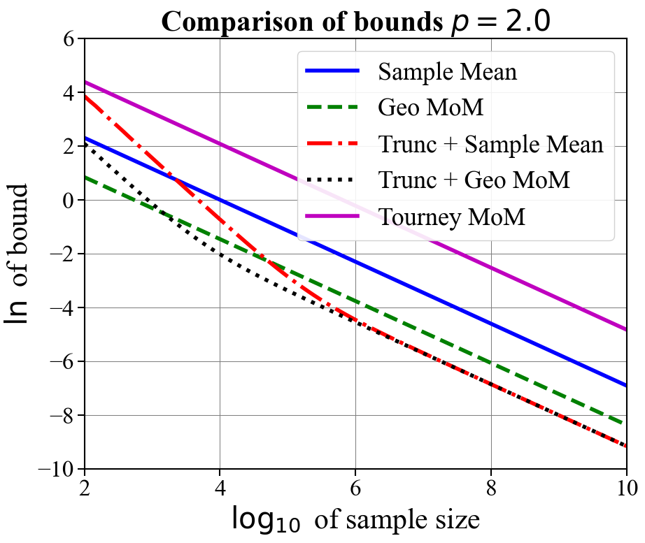
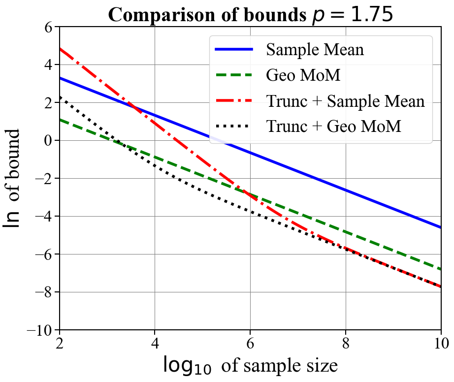
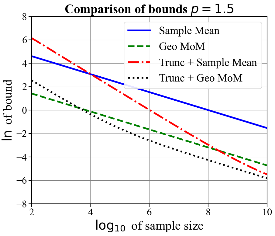
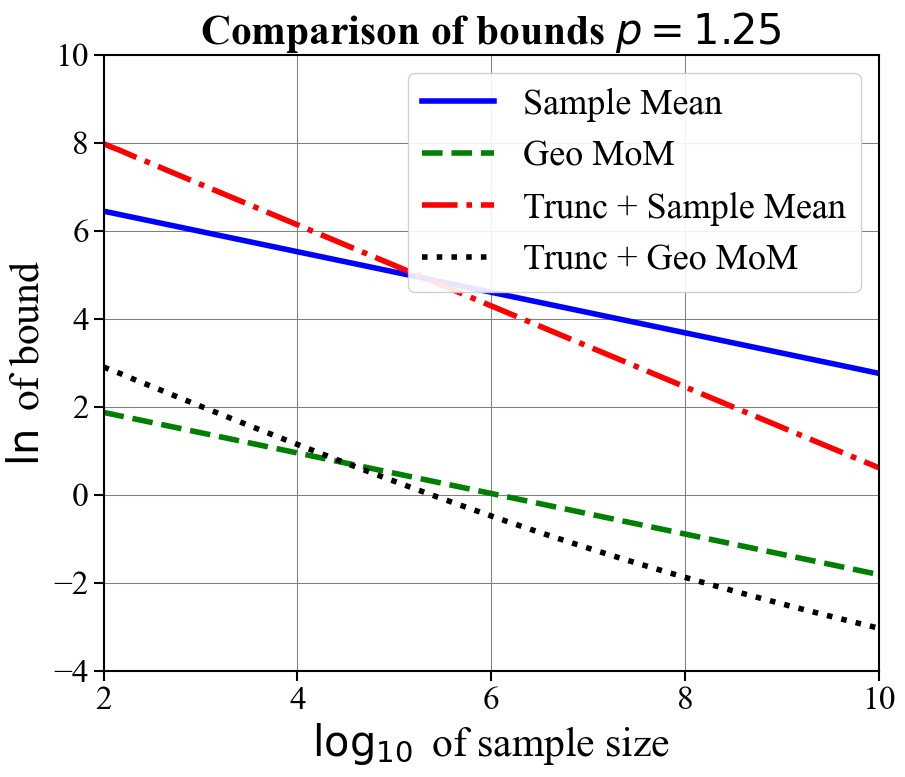
In Figure 1, we compare the confidence bounds obtained for our truncation-based estimators optimized for a fix sample size (Corollary 2.3) against other bounds in the literature. Namely, we compare against geometric median-of-means [33], the sample mean, and (in the case a shared covariance matrix exists for observations) the tournament median-of-means estimator [28]. We plot the natural logarithm of the bounds against the logarithm base ten of the sample sizes $n$ for $n\in[10^{2},10^{10}]$ and for $p\in\{1.25,1.5,1.75,2.0\}$ . We assume $\delta=10^{-4}$ and $v=1$ . For truncation-based estimates, we assume $k=\lfloor n/10\rfloor$ samples are used to produce the initial mean estimate and the remaining $n-k$ are used for the final mean estimate. We plot the resulting bounds for when the initial mean estimate is either computed using the sample mean or geometric median-of-means. For the tournament median-of-means estimate, we assume observations take their values in $\mathbb{R}^{d}$ for $d=100$ , and that the corresponding covariance matrix is the identity $\Sigma=I_{d}/d$ .

As expected, all bounds have a slope of $-(p-1)/p$ when $n$ is large, indicating equivalent dependence on the sample size. For all values of $p$ , the truncation-based estimator using geometric median-of-means as an initial estimate obtains the tightest rate once moderate sample sizes are reached ( $n=10^{4}$ or $n=10^{5}$ ). When $p\in\{1.25,1.5\}$ , much larger sample sizes are needed for truncation-based estimates with a sample mean initial estimate to outperform geometric median means (needing $\geq 10^{10}$ samples for $p=1.25$ ). For $p=2.0$ (i.e., finite variance) the tournament median-of-means estimate, despite achieving optimal sub-Gaussian dependence on $\lambda_{\max}(\Sigma)$ and $\Tr(\Sigma)=v$ , performs worse than even the naive mean estimate. This is due to prohibitively large constants. These plots suggest that the truncation-based estimate is a practical and computationally efficient alternative to approaches based on median-of-means.

Performance of Estimators on Simulated Data

In Figure 2, we examine the performance of the various mean estimators by plotting the distance between the estimates and the true mean. To do this, we sample $n=100,000$ i.i.d. samples $X_{1},\dots,X_{n}\in\mathbb{R}^{d}$ for $d=10$ in the following way. First, we sample i.i.d. directions $U_{1},\dots,U_{n}\sim\mathrm{Unif}(\mathbb{S}^{d-1})$ from the unit sphere. Then, we sample i.i.d. magnitudes $Y_{1},\dots,Y_{n}\sim\mathrm{Pareto}(a)$ from the Pareto II (or Lomax) distribution with $a=1.75$ .¹¹1If $Y\sim\mathrm{Pareto}(a)$ , the $Y$ has inverse polynomial density $\propto(1+x)^{-a}$ . The learner then observes $X_{1}=Y_{1}\cdot U_{1},\dots,X_{n}=Y_{n}\cdot U_{n}$ , and constructs either a geometric median estimate, a sample mean estimate, or a truncated mean estimate.

To compute the number of folds for geometric median-of-means, we follow the parameter settings outlined in Minsker [33] and assume a failure probability of $\delta=10^{-4}$ (although we are not constructing confidence intervals, the failure probability guides how to optimize the estimator). See Appendix B for further discussion on this estimator. Once again, we consider the truncated mean estimator centered at both the sample mean and a geometric median-of-means estimate. We always use $k=\lfloor\sqrt{n}\rfloor$ samples to construct the initial estimate, and produce a plot for hyperparameter $\lambda\in[0.0005,0.005,0.05,0.5]$ .

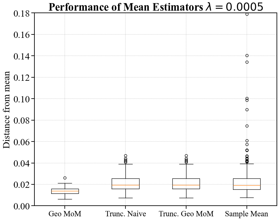
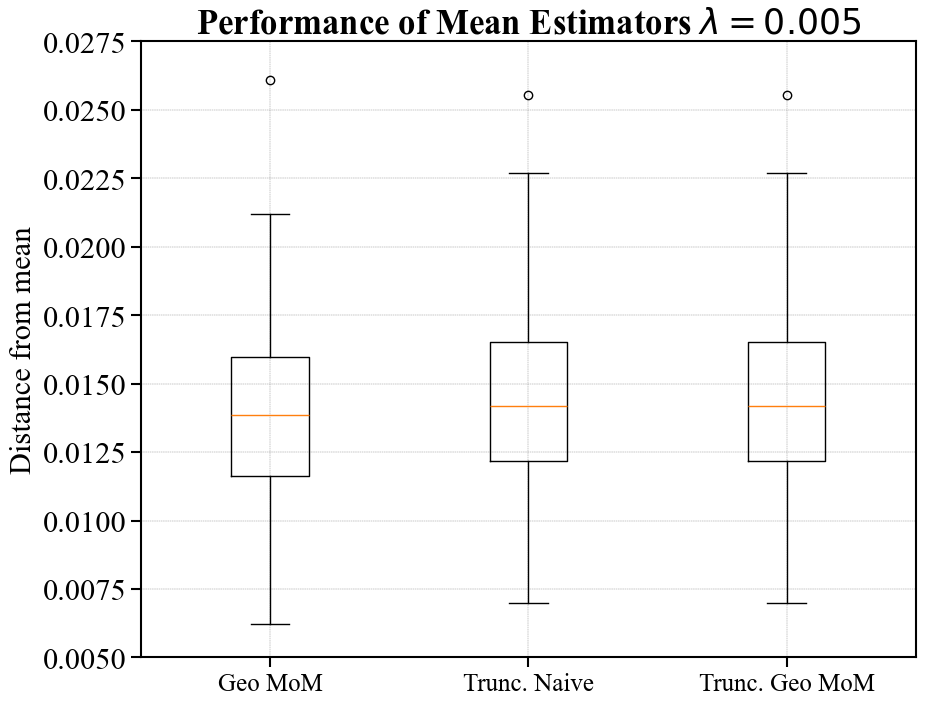
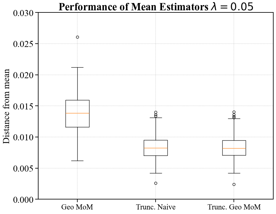
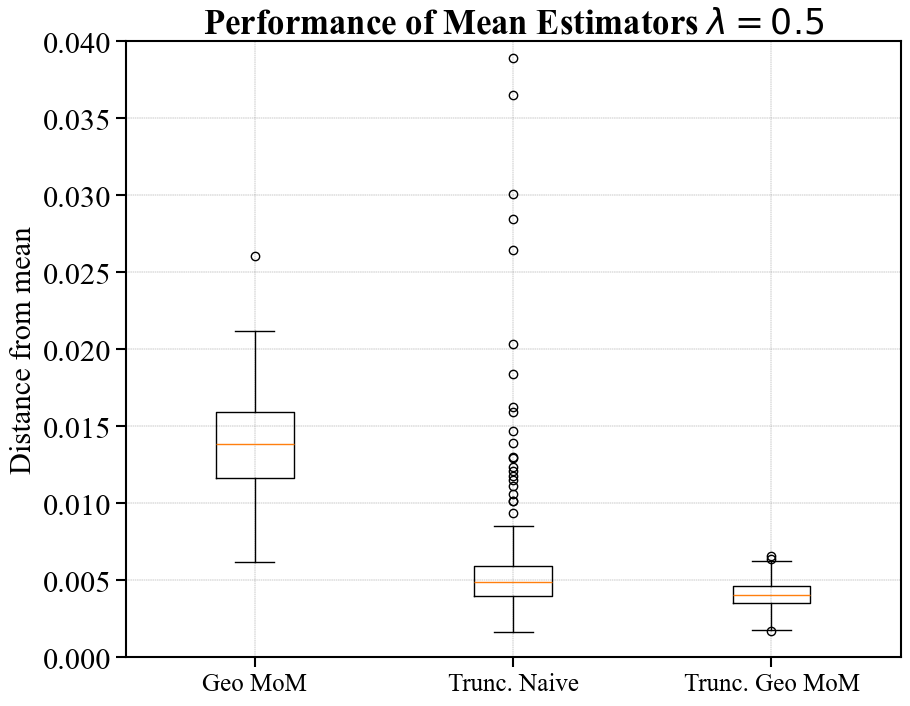
We construct these estimators over 250 independent runs and then construct box and whisker plots summarizing the empirical distance between the estimators and the true mean. The boxes have as a lower bound the first quartile $Q1$ , in the middle the sample median $M$ , and at the top the third quartile $Q3$ . The whiskers of the plot are given by the largest and smallest point falling within $M\pm 1.5\times(Q3-Q2)$ , respectively. All other points are displayed as outliers. We only include the sample mean in the first plot as to not compress the empirical distributions associated with other estimates.

As expected, the sample mean suffers heavily from outliers. For $\lambda\in\{0.0005,0.005\}$ (corresponding to truncation at large radii), the geometric median-of-means estimate is roughly two times closer to the mean than either truncation-based estimate. In the setting of aggressive truncation ( $\lambda\in\{0.05,0.5\}$ ), the truncated mean estimator centered at the geometric median-of-means initial estimate offers a significantly smaller distance to the true mean than just geometric median-of-means alone. The truncated estimate centered at the sample mean performs similarly for $\lambda=0.05$ , but suffers heavily from outliers when $\lambda=0.5$ . Interestingly, the recommended truncation level for optimizing tightness at $n=100,000$ samples is $\lambda\approx 0.0004$ per Corollary 2.2. Our experiments reflect that one may want to truncate more aggressively than is recommended in the corollary. In practice, one could likely choose an appropriate truncation level through cross-validation.

6 Summary

In this work, we presented a novel analysis of a simple truncation/threshold-based estimator of a heavy-tailed mean in smooth Banach spaces, strengthening the guarantees on such estimators that currently exist in the literature. In particular, we allow for martingale dependence between observations, replace the assumption of finite variance with a finite $p$ -th moment for $1<semantics><mrow><mn>1</mn><mo><</mo><mi>p</mi><mo>≤</mo><mn>2</mn></mrow><annotation encoding=$ , and let the centered $p$ -th moment be bounded instead of the raw $p$ -th moment (thus making the estimator translation invariant). Our bounds are also time-uniform, meaning they hold simultaneously for all sample sizes. We provide both a line-crossing inequality that can be optimized for a particular sample size (but remains valid at all times), and a bound whose width shrinks to zero at an iterated logarithm rate. Experimentally, our estimator performs quite well compared to more computationally intensive methods such as geometric median-of-means, making it an appealing choice for practical problems.

References

Abbasi-Yadkori [2013] Yasin Abbasi-Yadkori. Online learning for linearly parametrized control problems. PhD thesis, University of Alberta, 2013.
Alon et al. [1996] Noga Alon, Yossi Matias, and Mario Szegedy. The space complexity of approximating the frequency moments. In Proceedings of the Twenty-Eighth Annual ACM Symposium on Theory of Computing, pages 20–29, 1996.
Bubeck et al. [2013] Sébastien Bubeck, Nicolo Cesa-Bianchi, and Gábor Lugosi. Bandits with heavy tail. IEEE Transactions on Information Theory, 59(11):7711–7717, 2013.
Catoni [2007] Olivier Catoni. PAC-Bayesian supervised classification: the thermodynamics of statistical learning. arXiv preprint arXiv:0712.0248, 2007.
Catoni and Giulini [2017] Olivier Catoni and Ilaria Giulini. Dimension-free PAC-Bayesian bounds for matrices, vectors, and linear least squares regression. arXiv preprint arXiv:1712.02747, 2017.
Catoni and Giulini [2018] Olivier Catoni and Ilaria Giulini. Dimension-free PAC-Bayesian bounds for the estimation of the mean of a random vector. arXiv preprint arXiv:1802.04308, 2018.
Chen et al. [2021] Peng Chen, Xinghu Jin, Xiang Li, and Lihu Xu. A generalized Catoni’s M-estimator under finite $\alpha$ -th moment assumption with $\alpha\in(1,2)$ . Electronic Journal of Statistics, 15(2):5523–5544, 2021.
Cherapanamjeri et al. [2019] Yeshwanth Cherapanamjeri, Nicolas Flammarion, and Peter L Bartlett. Fast mean estimation with sub-Gaussian rates. In Conference on Learning Theory, pages 786–806. PMLR, 2019.
Cholaquidis et al. [2024] Alejandro Cholaquidis, Emilien Joly, and Leonardo Moreno. GROS: A general robust aggregation strategy. arXiv preprint arXiv:2402.15442, 2024.
Chowdhury and Gopalan [2017] Sayak Ray Chowdhury and Aditya Gopalan. On kernelized multi-armed bandits. In International Conference on Machine Learning, pages 844–853. PMLR, 2017.
Chugg et al. [2023a] Ben Chugg, Hongjian Wang, and Aaditya Ramdas. Time-uniform confidence spheres for means of random vectors. arXiv preprint arXiv:2311.08168, 2023a.
Chugg et al. [2023b] Ben Chugg, Hongjian Wang, and Aaditya Ramdas. A unified recipe for deriving (time-uniform) PAC-Bayes bounds. Journal of Machine Learning Research, 24(372):1–61, 2023b.
de la Peña et al. [2004] Victor H de la Peña, Michael J Klass, and Tze Leung Lai. Self-normalized processes: exponential inequalities, moment bounds and iterated logarithm laws. The Annals of Probability, 32(3), 2004.
de la Peña et al. [2007] Victor H de la Peña, Michael J Klass, and Tze Leung Lai. Pseudo-maximization and self-normalized processes. Probability Surveys, 4:172–192, 2007.
Gupta et al. [2024] Shivam Gupta, Samuel Hopkins, and Eric Price. Beyond Catoni: Sharper rates for heavy-tailed and robust mean estimation. In The Thirty Seventh Annual Conference on Learning Theory, pages 2232–2269. PMLR, 2024.
Hartman and Wintner [1941] Philip Hartman and Aurel Wintner. On the law of the iterated logarithm. American Journal of Mathematics, 63(1):169–176, 1941.
Hopkins [2020] Samuel B Hopkins. Mean estimation with sub-Gaussian rates in polynomial time. The Annals of Statistics, 48(2):1193–1213, 2020.
Howard et al. [2020] Steven R Howard, Aaditya Ramdas, Jon McAuliffe, and Jasjeet Sekhon. Time-uniform Chernoff bounds via nonnegative supermartingales. Probability Surveys, 17:257–317, 2020.
Howard et al. [2021] Steven R Howard, Aaditya Ramdas, Jon McAuliffe, and Jasjeet Sekhon. Time-uniform, nonparametric, nonasymptotic confidence sequences. The Annals of Statistics, 49(2):1055–1080, 2021.
Hsu and Sabato [2016] Daniel Hsu and Sivan Sabato. Loss minimization and parameter estimation with heavy tails. Journal of Machine Learning Research, 17(18):1–40, 2016.
Huber [1981] Peter J Huber. Robust statistics. Wiley Series in Probability and Mathematical Statistics, 1981.
Jerrum et al. [1986] Mark R Jerrum, Leslie G Valiant, and Vijay V Vazirani. Random generation of combinatorial structures from a uniform distribution. Theoretical Computer Science, 43:169–188, 1986.
Kesten [1972] Harry Kesten. The 1971 rietz lecture sums of independent random variables–without moment conditions. The Annals of Mathematical Statistics, pages 701–732, 1972.
Langford and Shawe-Taylor [2002] John Langford and John Shawe-Taylor. PAC-Bayes & margins. Advances in Neural Information Processing Systems, 15, 2002.
Ledoux and Talagrand [2013] Michel Ledoux and Michel Talagrand. Probability in Banach Spaces: Isoperimetry and processes. Springer Science & Business Media, 2013.
Lugosi and Mendelson [2019a] Gábor Lugosi and Shahar Mendelson. Mean estimation and regression under heavy-tailed distributions: A survey. Foundations of Computational Mathematics, 19(5):1145–1190, 2019a.
Lugosi and Mendelson [2019b] Gábor Lugosi and Shahar Mendelson. Near-optimal mean estimators with respect to general norms. Probability theory and related fields, 175(3):957–973, 2019b.
Lugosi and Mendelson [2019c] Gábor Lugosi and Shahar Mendelson. Sub-Gaussian estimators of the mean of a random vector. The Annals of Statistics, 47(2):783–794, 2019c.
Lugosi and Mendelson [2021] Gabor Lugosi and Shahar Mendelson. Robust multivariate mean estimation: the optimality of trimmed mean. Annals of Statistics, 2021.
Maller [1980] RA Maller. On the law of the iterated logarithm in the infinite variance case. Journal of the Australian Mathematical Society, 30(1):5–14, 1980.
Martinez-Taboada and Ramdas [2024] Diego Martinez-Taboada and Aaditya Ramdas. Empirical Bernstein in smooth Banach spaces. arXiv preprint arXiv:2409.06060, 2024.
Mathieu [2022] Timothée Mathieu. Concentration study of M-estimators using the influence function. Electronic Journal of Statistics, 16(1):3695–3750, 2022.
Minsker [2015] Stanislav Minsker. Geometric median and robust estimation in Banach spaces. Bernoulli, pages 2308–2335, 2015.
Nemirovskij and Yudin [1983] Arkadij Semenovič Nemirovskij and David Borisovich Yudin. Problem complexity and method efficiency in optimization. 1983.
Oliveira and Orenstein [2019] Roberto I Oliveira and Paulo Orenstein. The sub-Gaussian property of trimmed means estimators. Technical Report, IMPA, 2019.
Pinelis [1992] Iosif Pinelis. An approach to inequalities for the distributions of infinite-dimensional martingales. In Probability in Banach Spaces, 8: Proceedings of the Eighth International Conference, pages 128–134. Springer, 1992.
Pinelis [1994] Iosif Pinelis. Optimum bounds for the distributions of martingales in Banach spaces. The Annals of Probability, pages 1679–1706, 1994.
Ramdas and Wang [2024] Aaditya Ramdas and Ruodu Wang. Hypothesis testing with e-values. arXiv preprint arXiv:2410.23614, 2024.
Robbins [1970] Herbert Robbins. Statistical methods related to the law of the iterated logarithm. The Annals of Mathematical Statistics, 41(5):1397–1409, 1970.
Tukey and McLaughlin [1963] John W Tukey and Donald H McLaughlin. Less vulnerable confidence and significance procedures for location based on a single sample: Trimming/winsorization 1. Sankhyā: The Indian Journal of Statistics, Series A, pages 331–352, 1963.
Ville [1939] Jean Ville. Etude critique de la notion de collectif. Gauthier-Villars Paris, 1939.
Wang and Ramdas [2023] Hongjian Wang and Aaditya Ramdas. Catoni-style confidence sequences for heavy-tailed mean estimation. Stochastic Processes and Their Applications, 163:168–202, 2023.
Whitehouse et al. [2023a] Justin Whitehouse, Aaditya Ramdas, and Steven Z Wu. On the sublinear regret of GP-UCB. Advances in Neural Information Processing Systems, 36:35266–35276, 2023a.
Whitehouse et al. [2023b] Justin Whitehouse, Zhiwei Steven Wu, and Aaditya Ramdas. Time-uniform self-normalized concentration for vector-valued processes. arXiv preprint arXiv:2310.09100, 2023b.

Appendix A Omitted Proofs

Proof of Corollary 2.2.

Taking $\lambda$ as in (2.7) it’s easy to see that the width obeys

\|\widehat{\mu}_{n}(k)-\mu\|\leq\Big{(}(\mathfrak{C}_{p}(\mathbb{B})+K_{p}2^{p-1})(v+r(\delta_{2},k)^{p})\Big{)}^{1/p}\left(\frac{\log(2/\delta_{1})}{n-k}\right)^{(p-1)/p}.

If $k=o(n)$ we have $(\log(2/\delta_{1})/(n-k))^{(p-1)/p}=(\log(2/\delta_{1})/n)^{(p-1)/p}$ and if $r(\delta_{2},k)=o(1)$ then $v+r(\delta_{2},k)^{p}=O(v)$ . Further, if $\delta_{1}=O(\delta)$ then $\log(2/\delta_{1})=O(\log(1/\delta))$ . So under these conditions we have

\|\widehat{\mu}_{n}(k)-\mu\|=O\left(v^{1/p}\left(\frac{\log(1/\delta)}{n}\right)^{1-1/p}\right),

as desired. ∎

Proof of Corollary 2.3.

Let $\widehat{Z}_{k}$ be the empirical mean on the first $k-1$ observations. By Markov and Jensen’s inequality,

	$\displaystyle\mathbb{P}(\\|\widehat{Z}_{k}-\mu\\|\geq r)$	$\displaystyle\leq\frac{\mathbb{E}\\|\widehat{Z}-\mu\\|^{p}}{r^{p}}=\frac{\mathbb{E}\\|\frac{1}{k-1}\sum_{i\leq k-1}(X_{i}-\mu)\\|^{p}}{r^{p}}$
		$\displaystyle\leq\frac{\sum_{i}\mathbb{E}\\|X_{i}-\mu\\|^{p}}{(k-1)^{p}r^{p}}\leq\frac{v}{(k-1)^{p-1}r^{p}}.$		(A.1)

Therefore, taking $r^{p}(\delta,k)=\frac{v}{\delta(k-1)^{p-1}}$ suffices to guarantee that $\mathbb{P}(\|\widehat{Z}_{k}-\mu\|\geq r(\delta,k))\leq\delta$ . Using the binomial expansion (and assuming $k$ is large enough such that $\delta_{2}k^{p-1}\geq 1$ ), write

	$\displaystyle\left(1+\frac{1}{\delta_{2}(k-1)^{p-1}}\right)^{1/p}$	$\displaystyle=1+\frac{1}{p\delta_{2}(k-1)^{p-1}}+O\left(\frac{1}{(\delta_{2}(k-1)^{p-1})^{2}}\right)$
		$\displaystyle=1+O\left(\frac{1}{\delta_{2}k^{p-1}}\right).$

Therefore, taking $\lambda$ as in (2.7) and applying Corollary 2.2, with probability $1-\delta$ ,

	$\displaystyle\\|\widehat{\mu}_{n}(k)-\mu\\|$	$\displaystyle\leq\Big{(}C_{p}(v+r(\delta_{2},k)^{p})\Big{)}^{1/p}\left(\frac{\log(2/\delta_{1})}{n-k}\right)^{(p-1)/p}$
		$\displaystyle=v^{1/p}C_{p}^{1/p}\left(1+O\left(\frac{1}{\delta_{2}k^{p-1}}\right)\right)\left(\frac{\log(2/\delta_{1})}{n-k}\right)^{(p-1)/p},$

as claimed. For the proof of (2.10), we use a very similar argument but use the error rate of geometric median-of-means given in Appendix B. In particular, in this case we may take

r(\delta,k)=O\left(v^{1/p}\left(\frac{\log(1/\delta)}{k}\right)^{1-1/p}\right),

which, when plugged into the previous display, gives the desired result. ∎

Appendix B Geometric Median-of-Means in Banach Spaces

While Minsker [33] studied mean estimation in smooth Banach spaces, his examples weren’t stated explicitly for Banach spaces nor for the case of infinite variance. Here we show that his geometric median-of-means estimator, when paired with empirical mean, achieves rate $O(v^{1/p}(\log(1/\delta)/n)^{\frac{p-1}{p}})$ , the same as our rate.

Minsker [33, Theorem 3.1] provides the following bound. Let $\widehat{\mu}_{1},\dots,\widehat{\mu}_{B}$ be a collection of independent estimators of the mean $\mu$ . Fix $\alpha\in(0,1/2)$ . Let $0<\gamma<\alpha$ and $\epsilon>0$ be such that for all $b$ , $1\leq b\leq B$ , we have

\mathbb{P}(\|\mu-\widehat{\mu}_{b}\|>\epsilon)\leq\gamma.

(B.1)

Let $\widehat{\mu}=\text{median}(\widehat{\mu}_{1},\dots,\widehat{\mu}_{B})$ be the geometric median, defined as

\widehat{\mu}:=\arg\min_{\mu\in\mathbb{B}}\sum_{b=1}^{B}\|\widehat{\mu}_{b}-\mu\|.

Then

\mathbb{P}(\|\mu-\widehat{\mu}\|>C_{\alpha}\epsilon)\leq\exp(-B\psi(\alpha;\gamma)),

(B.2)

where

\psi(\alpha;\gamma)=(1-\alpha)\log\frac{1-\alpha}{1-\gamma}+\alpha\log\frac{\alpha}{\gamma},

and

C_{\alpha}=\frac{2(1-\alpha)}{1-2\alpha}.

We will optimize Minsker’s bound by taking the same optimization parameters as in his paper. That is, we will set $\alpha_{\ast}:=\frac{7}{18}$ and $\gamma_{\ast}:=0.1$ and will set the number of naive mean estimators $B$ to be given by

B:=\left\lfloor\frac{\log(1/\delta)}{\psi(\alpha_{\ast};\gamma_{\ast})}\right\rfloor+1\leq 3.5\log(1/\delta)+1,

which provides an overall failure probability of at most $\exp(-B\psi(\alpha_{\ast};\gamma_{\ast}))\leq\delta.$ Markov’s and Jensen’s inequalities (as in Appendix A, see (A.1)) together yield

\mathbb{P}(\|\widehat{\mu}_{b}-\mu\|\geq\epsilon)\leq\frac{v}{\epsilon^{p}(n/B)^{p-1}}\leq\gamma_{\ast},

if we take

\epsilon=\left(\frac{B^{p-1}v}{\gamma n^{p-1}}\right)^{1/p}.

Therefore, we obtain that with probability $1-\delta$ ,

\displaystyle\|\widehat{\mu}-\mu\|

\displaystyle\leq C_{\alpha_{\ast}}\epsilon=\frac{2(1-\alpha_{\ast})}{1-2\alpha_{\ast}}\left(\frac{B^{p-1}}{\gamma_{\ast}n^{p-1}}\right)^{1/p}v^{1/p}\leq\frac{5.5}{0.1^{1/p}}v^{1/p}\left(\frac{3.5\log(1/\delta)+1}{n}\right)^{1-1/p}.

Appendix C Noncentral moment bounds

For completeness, we state our bound when we assume only a bound on the raw (uncentered) $p$ -th moment of the observations. This was the setting studied by Catoni and Giulini [6]. We replace assumption 1 with the following:

Assumption 3.

We assume $(X_{n})_{n\geq 1}$ are a sequence of $\mathbb{B}$ -valued random variables adapted to a filtration $(\mathcal{F}_{n})_{n\geq 0}$ such that

(1)

$\mathbb{E}(X_{n}\mid\mathcal{F}_{n-1})=\mu$ , for all $n\geq 1$ and some unknown $\mu\in\mathbb{B}$ , and
(2)

$\sup_{n\geq 1}\mathbb{E}\left(\|X_{n}\|^{p}\mid\mathcal{F}_{n-1}\right)\leq v<\infty$ for some known $p\in(1,2]$ and some known constant $v>0$ .

With only the raw moment assumption, we do not try and center our estimator. Instead we deploy $\widehat{\mu}_{n}(0,\lambda,0)=\frac{1}{n}\sum_{m\leq n}\mathtt{Trunc}(\lambda X_{m})X_{m}$ . With this estimator we obtain the following result, which achieves the same rate as Catoni and Giulini [6] and Chugg et al. [11].

Theorem C.1.

Let $X_{1},X_{2},\dots$ be random variables satisfying Assumption 3 which live in some Banach space $(\mathbb{B},\|\cdot\|)$ satisfying Assumption 2. Fix any $\delta\in(0,1]$ . Then, for any $\lambda>0$ , with probability $1-\delta$ , simultaneously for all $n\geq 1$ , we have:

\left\|\widehat{\mu}_{n}(0,\lambda,0)-\mu\right\|\leq 2v\lambda^{p-1}(\mathfrak{C}_{p}(\mathbb{B})+K_{p}2^{p-1})+\frac{\log(2/\delta)}{\lambda n}.

(C.1)

Moreover, if we want to optimize the bound at a particular sample size $n^{*}$ and we set

\lambda=\left(\frac{\log(2/\delta)}{2n^{*}v(\mathfrak{C}_{p}(\mathbb{B})+K_{p}2^{p-1})}\right)^{1/p},

then with probability $1-\delta$ ,

\left\|\widehat{\mu}_{n}(0,\lambda,0)-\mu\right\|\leq(2v(\mathfrak{C}_{p}(B)+K_{p}2^{p-1}))^{1/p}\left(\frac{\log(1/\delta)}{n}\right)^{1-1/p}.

(C.2)

Proof.

Apply Theorem 2.1 with $k=0$ and $\widehat{Z}_{k}=0$ . Then note that we can take $r(\delta,0)=v^{1/p}$ for all $\delta$ since $\|\mu\|\leq(\mathbb{E}\norm{X}^{p})^{1/p}\leq v^{1/p}$ by Jensen’s inequality. ∎

	$\displaystyle\\|\mu-\widetilde{\mu}_{n}(\lambda)\\|$	$\displaystyle=\\|\mathbb{E}_{n-1}[X_{n}]-\mathbb{E}_{n-1}[\mathtt{Trunc}(\lambda(X_{n}-z))(X_{n}-z)+z]\\|$
		$\displaystyle=\\|\mathbb{E}_{n-1}[\{1-\mathtt{Trunc}(\lambda(X_{n}-z))\}(X_{n}-z)\\|$
		$\displaystyle\leq\mathbb{E}[\|1-\mathtt{Trunc}(\lambda(X_{n}-z))\|^{q}]^{1/q}\mathbb{E}[\\|X_{n}-z\\|^{p}]^{1/p},$

$\displaystyle\mathbb{E}_{n-1}[\\|X_{n}-z\\|^{p}]$	$\displaystyle=\mathbb{E}_{n-1}[\\|X_{n}-\mu+\mu-z\\|^{p}]$
	$\displaystyle\leq 2^{p-1}\left(\mathbb{E}_{n-1}[\\|X_{n}-\mu\\|^{p}]+\\|z-\mu\\|^{p}\right)$
	$\displaystyle\leq 2^{p-1}(v+\\|z-\mu\\|^{p}).$	(3.5)

$\displaystyle\mathbb{E}_{n-1}\\|\Delta S_{n}\\|^{2}$	$\displaystyle\leq C\lambda_{n}^{2}\mathbb{E}_{n-1}\left[\\|T_{n}\\|^{p}\\|T_{n}\\|^{2-p}\right]$
	$\displaystyle\leq C\lambda_{n}^{p}\mathbb{E}_{n-1}\left\\|T_{n}\right\\|^{p}$
	$\displaystyle\leq C\lambda_{n}^{p}\mathbb{E}_{n-1}\left\\|Y_{n}\right\\|^{p}$
	$\displaystyle\leq C\lambda_{n}^{p}2^{p-1}(v+\\|\mu-\widehat{Z}_{n}\\|^{p}),$	(3.8)

	$\displaystyle\varphi^{\prime}(0)$	$\displaystyle=\frac{d}{dt}\left(\mathbb{E}_{n-1}\cosh(\\|S_{n-1}+t\Delta S_{n}\\|)\right)\big{\|}_{t=0}$
		$\displaystyle=\mathbb{E}_{n-1}\left[\frac{d}{dt}\cosh(\\|S_{n-1}+t\Delta S_{n}\\|)\Big{\|}_{t=0}\right]$
		$\displaystyle=\mathbb{E}_{n-1}\left[\langle D_{f}\\|f\\|\big{\|}_{f=S_{n-1}},\Delta S_{n}\rangle\cdot\frac{d}{dx}\cosh(x)\big{\|}_{x=\\|S_{n-1}\\|}\right]$
		$\displaystyle=\left\langle D_{f}\\|f\\|\big{\|}_{f=S_{n-1}},\mathbb{E}_{n-1}\Delta S_{n}\right\rangle\cdot\frac{d}{dx}\cosh(x)\big{\|}_{x=\\|S_{n-1}\\|}$
		$\displaystyle=0,$

	$\displaystyle\mathbb{E}_{n-1}\cosh(\\|S_{n}\\|)$	$\displaystyle=\varphi(0)+\varphi^{\prime}(0)+\int_{0}^{1}(1-\theta)\varphi^{\prime\prime}(\theta)d\theta$
		$\displaystyle\leq\cosh(\\|S_{n-1}\\|)\left(1+\beta^{2}\mathbb{E}_{n-1}\left[\\|\Delta S_{n}\\|^{2}\right]\int_{0}^{1}(1-\theta)e^{2\theta}d\theta\right)$
		$\displaystyle\stackrel{{\scriptstyle(i)}}{{\leq}}\cosh(\\|S_{n-1}\\|)\left(1+\beta^{2}\left(\frac{e^{2}-3}{4}\right)\mathbb{E}_{n-1}\left[\\|\Delta S_{n}\\|^{2}\right]\right)$
		$\displaystyle\stackrel{{\scriptstyle(ii)}}{{\leq}}\cosh(\\|S_{n-1}\\|)\left(1+\mathfrak{C}_{p}(\mathbb{B})\lambda_{n}^{p}(v+\\|\mu-\widehat{Z}_{n}\\|^{p})\right)$
		$\displaystyle\stackrel{{\scriptstyle(iii)}}{{\leq}}\cosh(\\|S_{n-1}\\|)\exp\left\{\mathfrak{C}_{p}(\mathbb{B})\lambda_{n}^{p}(v+\\|\mu-\widehat{Z}_{n}\\|^{p})\right\},$

Mean Estimation in Banach Spaces Under Infinite Variance and Martingale Dependence

Abstract

1 Introduction

1.1 Our Contributions

1.2 Related Work

Heavy-tailed mean estimation under independent observations.

Sequential concentration under martingale dependence.

Concentration in Hilbert and Banach Spaces.

1.3 Preliminaries

Assumption 1.

Assumption 2.

Notation and background.

Outline.

2 Main Result

Theorem 2.1 (Main result).

Corollary 2.2.

Corollary 2.3.

3 Proof of Theorem 2.1

3.1 Step 1: Bounding ‖μ~n​(λ)−μ‖\|\widetilde{\mu}_{n}(\lambda)-\mu\|

Lemma 3.1.

Proof.

Lemma 3.2.

Proof.

3.2 Step 2: Bounding ‖ξ^n​(λn)−∑m≤nλm​μ~m​(λm)‖\|\widehat{\xi}_{n}(\lambda^{n})-\sum_{m\leq n}\lambda_{m}\widetilde{\mu}_{m}(\lambda_{m})\|

Proposition 3.3.

Proof.

3.3 Step 3: Bounding Mn​(λn)M_{n}(\lambda^{n})

Lemma 3.4.

Proof.

Proposition 3.5.

Proof.

Proof of Theorem 2.1.

4 Law of the Iterated Logarithm Rates

Theorem 4.1 (Stitching).

Proof of Theorem 4.1.

5 Bound Comparison and Simulations

Comparing Tightness of Bounds

Performance of Estimators on Simulated Data

6 Summary

References

Appendix A Omitted Proofs

Proof of Corollary 2.2.

Proof of Corollary 2.3.

Appendix B Geometric Median-of-Means in Banach Spaces

Appendix C Noncentral moment bounds

Assumption 3.

Theorem C.1.

Proof.

Mean Estimation in Banach Spaces
Under Infinite Variance and Martingale Dependence

3.1 Step 1: Bounding $\|\widetilde{\mu}_{n}(\lambda)-\mu\|$

3.2 Step 2: Bounding $\|\widehat{\xi}_{n}(\lambda^{n})-\sum_{m\leq n}\lambda_{m}\widetilde{\mu}_{m}(\lambda_{m})\|$

3.3 Step 3: Bounding $M_{n}(\lambda^{n})$