MöbiusE: Knowledge Graph Embedding on Möbius Ring
Abstract
In this work, we propose a novel Knowledge Graph Embedding (KGE) strategy, called MöbiusE, in which the entities and relations are embedded to the surface of a Möbius ring. The proposition of such a strategy is inspired by the classic TorusE, in which the addition of two arbitrary elements is subject to a modulus operation. In this sense, TorusE naturally guarantees the critical boundedness of embedding vectors in KGE. However, the nonlinear property of addition operation on Torus ring is uniquely derived by the modulus operation, which in some extent restricts the expressiveness of TorusE. As a further generalization of TorusE, MöbiusE also uses modulus operation to preserve the closeness of addition operation on it, but the coordinates on Möbius ring interacts with each other in the following way: any vector on the surface of a Möbius ring moves along its parametric trace will goes to the right opposite direction after a cycle. Hence, MöbiusE assumes much more nonlinear representativeness than that of TorusE, and in turn it generates much more precise embedding results. In our experiments, MöbiusE outperforms TorusE and other classic embedding strategies in several key indicators.
keywords:
Möbius ring, Torus ring , Knowledge graph , Embedding1 Introduction
Graph or network structure can usually be used to model the intrinsic information behind data [1]. As an typical example, a knowledge graph (KG) is a collection of facts of the real world, related examples include DBpedia [2], YAGO [3] and Freebase [4]. These built KG database can be applied in many realistic engineering tasks, such as knowledge inference, question answering, and sample labeling. Driven by realistic applications, an intriguing and challenging problem for KG is: how to infer those unknown knowledge (or missing data) via the existing built KG database.
For any KG, the basic element of knowledge is represented by a triplet , which composed of two entities and one relation . In detail, is called the head, is called the tail, and means head maps to tail via the operation of relation . For example, the entity U.S.A projects to DonaldTrump under the relation ThePresidentOf, and the entity U.S.A projects to MikePence under the relation TheVicePresidentOf. Based on these two triplets, and considering the fact of “the president and vice president of a country at the same time are colleagues”, one predicts the existence of the triplet DonaldTrump, IsColleagueOf, MikePence if such triplet is not contained in the given database. For realistic applications such as question answering, the core task is to predict those triplets which are not listed in the given database, such as task is called link prediction in KG.
There exists many types of method for link prediction in KG, among which translation-based methods treats each entity and relation as embedded vectors in some constructed algebraic space, and each true triplet can be translated to a simple constraint described by an algebraic expression . Using such a method, if some is not presented in KG but the corresponding algebraic constraint index is very small, then it is reasonable to believe that is a missing fact. Due to the choosing of different algebraic space, many different translation-based models have be obtained. TransE [5] is the first translation-based model for link prediction tasks, in which it uses the Euclidean space as the embedding space and the constraint quantity for each triplet is set as simple as . TransR [6] builds the constraint equation by mapping the entities to a subspace derived by the relation vector. TansH [7] improves TransE in dealing with reflexive/ONE-TO-MANY/MANY-TO-ONE/MANY-TO-MANY cases in KG, such an improvement is caused by treating each relation as a translating operation on a hyperplane. DistMult [8] utilizes a simple bilinear formulation to model the constraint generated by triplets, in this way the composition of relation is characterized by matrix multiplication, which makes such a model good at capturing relational semantics. ComplEx [9] uses the standard dot product between embeddings and demonstrates the capability of complex-valued embeddings instead of real-valued numbers. TorusE [10] chooses a compact Lie group, a torus, as the embedding space, and is more scalable to large-size knowledge graphs because of its lower computational complexity. Other types of embedding methods include TransA [11], a locally and temporally adaptive translation-based approach; ConvE [12], a multi-layer convolutional network embedding model; TransF, an embedding strategy with flexibility in each triplet constraint; QuaternionE [13], an embedding method treats each relation as a quaternion in hypercomplex space.
Among the above embedding methods, the basic operation behind TorusE is a simple modulus operation and this operation automatically regularizes the calculated results to the given bounded area. In this way, there is no need to make an extra regularization operation in TorusE. Inspired by this property of TorusE, we move beyond one-dimensional modulus operation on Lie group and propose MöbiusE, which takes a Möbius ring (whose basic dimension is two) as the embedding space. This MöbiusE has the following major benefits for embedding tasks: At first, MöbiusE provides much more flexibility since each point on the surface of a Möbius ring has two different expressions; Second, the expressiveness of MöbiusE is much greater than TorusE due to the complex distance function built in Möbius ring; Third, MöbiusE also automatically truncates the training vectors to constraint space as that of TorusE; Finally, MöbiusE subsumes TorusE, and inherits all the attractive properties of TorusE, such as its ability to model symmetry/antisymmetry, inversion, and composition.
The rest of the paper is organized as follows: Section 2 revisits the idea of TorusE and proposes the basic idea of MöbiusE, especially, we discuss about how to define the distance function on a Möbius ring. Section 3 provides the experiment results for MöbiusE on datasets FB15K and WN18. Section 4 discuss about related works and compare MöbiusE with other embedding methods. Section 5 concludes this paper. In the end, Section 6 lists the proof for several key propositions on Möbius ring.
2 Embedding on Möbius Ring
A KG is described by a set of triples , where each contains , , and as head entity, relation, and tail entity, respectively. Denote and as the set of entities and relations of . Let be the scoring function, the task of KGE is to find vectors corresponding to which minimize:
| (1) |
where
| (2) | |||||
| (3) | |||||
| (4) |
and , is a margin hyperparameter. The function is defined by for .
Suppose be a positive triple, the trueness of assessed by is given by
| (5) | |||||
In general, we use the value to evaluate the trueness of a candidate triplet.
In order to begin with the following description, we give two critical functions and .
For any and , is defined as111 is equivalent to in [10].
| (6) |
is defined as
| (7) |
Based on these definitions, for any , it is not difficult to verify that , , , and . In particular, can be reformulated as .
2.1 Revisit Torus Ring
Before introducing , we would like review the definition of Torus ring . As shown in Fig. 1, is a one-dimensional ring. In particular, any two points and on can be uniquely defined by their angles and with , these variables are all depicted in Fig. 1.
The addition operation of any two points and is defined by . The distance between and can be viewed as the minimal value among the rotating angles from to and from to , i.e., and as shown in Fig. 1. Describing such an idea in math, we have
This distance function (and all the following distance functions) satisfies
| (11) |
where .
Torus ring can be viewed as the independent stacking of two Torus ring . Given as two points on Torus ring , then the addition operation on is defined by . The distance function on is given as
where is some vector norm.
Torus ring can be extended to -dimensional case, let as two points on , it holds
| (12) | |||||
| (13) |
where
Summarize the above discussion, the objective function (1) becomes TorusE when the scoring function is set as

2.2 Möbius Ring
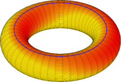
As an intuitive illustration of Möbius ring, we plot the surface of Möbius ring in Fig. 3. In this figure, let the radius from the center of the hole to the center of the tube be , the radius of the tube be , then the parametric equation for Möbius ring is
| (17) |
Letting and , then any point on can be uniquely defined by . In particular, the period of is and the period of is , hence we set .
Given as two points on a Möbius ring, the addition operation on is defined by
| (18) |
i.e., the addition on is formulated by the modulus addition on each dimension with modulus and , respectively.
The distance function between and is defined as
| (19) | |||||
| (20) | |||||
| (21) |
One can further verify that the above definition follows the basic properties in (11). Moreover, the above distance satisfies:
Proposition 1.
For distance defined in (19) for and any two points , in , it holds , where the upperbound achieves when and for some integer and .
We give the proof of Proposition 1 in Appendix 6.3. In what follows, we will explain the reason for the definition (19) by using equation (17).
Given and the corresponding points and on , transforming to (or, to ) needs one of the following two operations:
-
a).
If transform to , then add to the first component of , and add to the second component of for some integer and . If transform to , then add to the first component of , and add to the second component of for some integer and . Hence, when we measure the distance in the first dimension using modulus and considering that , such a distance is . Similarly, if we measure the distance between and in the second dimension using modulus and considering that , the obtained distance is . By adding the distance in the two dimensions, we simply obtain the distance in this case be , which conforms with (20).
-
b).
If transform to , then add to the first component of , and add to the second component of for some integer and . If transform to , then add to the first component of , and add to the second component of for some integer and . In order to make an intuitive calculation, we calculate the value of and for in (17) as
when add to , and add to , it becomes
which coincides with the coordinate of on (ignore multiple of difference). Similar calculation can be conducted for the case of transforming to and hence we omit the details. To sum it up, when we measure the distance in the first dimension using modulus and considering that , such a distance is . Similarly, if we measure the distance between and in the second dimension using modulus and considering that , the obtained distance is . By adding the distance in the two dimensions, we simply obtain the distance in this case be , which conforms with (21).
Summarize the above discussion, the distance between should be the minimum of the two cases, which is equivalent to (19).
In fact, Möbius ring degenerates to Torus ring in some special case, as shown in the following proposition, whose proof is given in Appendix 6.3.
Proposition 2.
If the first dimension of is set to zero, then is equivalent to .
For comparison between Torus ring and Möbius ring, we list the parametric equations for Torus ring as:
| (25) |
As we can see in (25), the period of and are both , hence the following points on are equivalent:
However, in Möbius (17), the period of and are and respectively. In particular, the following points can be viewed as equivalent points on Möbius ring:
which can be verified in (17).
As shown in Fig. 2 and Fig. 3, the parametric curve on Torus ring and Möbius ring are also quite different: fixing in (25) generates a cycle, but fixing in (17) generates a twisted cycle.

2.3 Möbius Ring
The simple Möbius ring can be extended to more general case . Möbius ring is a space constructed on , where are co-prime positive integers, any satisfies:
| (26) | |||||
| (27) | |||||
The reason of why is defined as (30) is similar to that of (19) and hence omitted here. The distance satisfies properties (11) too, and in particular there is:
Proposition 3.
The proof of the above proposition is similar to that of Proposition 1 and hence omitted in this paper. The proof of in in (11) is given in Appendix 6.1.
In order to increase the embedding dimensions for KGE, we define
| (28) |
as the direct sum of Möbius ring . For each , , there is for each and
| (29) | |||||
| (30) |
where and is some vector norm.
For embedding on Möbius ring, the scoring function in (1) will be set as
where the operation is defined in (29) and distance function is defined in (30), which is listed in Tab. 1.
In what follows, we list a key proposition for Möbius ring , whose proof is intuitive and hence omitted here.
Proposition 4.
The solutions of the following equation
| (31) |
in the region for are with and .
In the next, we call the solutions of equation (31) be zero points of .
For any given KG described by set of triplets , one of the difficulties for KGE comes from the cycle structure in the given KG data, a cycle structure in KG means the existence of entities and relations () such that
and or . In the case that the given set contains no cycle structure, the geometric structure of becomes a tree, and the embedding task for this KG without considering the negative samples can be implemented via a simple iteration strategy. However, realistic KG data contains a great amount of logic cycles and an appropriate KGE strategy should choose an algebraic structure which is capable of fitting the constraint generated by tremendous number of cycles.
Consider the properties in (11), the constraint of the above cycle without entities can be described by an equation of relations on :
| (32) |
where , .
In general, the number of cycles in a given KG dataset is much larger than that of the relations, hence the set of equations (32) in Euclidean space is hardly to have an exact solution. Intuitively, since the number of zero points in in the region is , the set of equations (32) derived by all the cycles in given KG data will have more chance to get an exact solution. However, the number of zero point in is only for TorusE, which is much smaller than that of . In the above sense, MöbiusE assumes more powerful expressiveness than TorusE.
3 Experiments
The performance of the proposed MöbiusE is tested on two datasets: FB15K and WN18 [5], which are extracted from realistic knowledge graphs. The basic properties on these two datasets is given in Tab. 2.
We conduct the link prediction task by using the same method reported in [5]. For each test triplet (which is a positive sample), we replace its head (or tail) to generate a corrupted triplet, then the score of each corrupted triplet is calculated by the scoring function , and the ranking of the test triplet is obtained according to these scores, i.e., the definition of in (5). It should be noted from (4) that the set of generated corrupted elements excludes the positive triplets , we call such a set be “filtered” [10], and the ranking values in our experiments are all obtained on the “filtered” set.
We choose stochastic gradient descent algorithm to optimize the objective (1). In order to generate the negative sample in (1), we employ the “Bern” method [7] for negative sampling because of the datasets only contains positive triplets.
To evaluate our model, we use Mean Rank (MR), Mean Reciprocal Rank (MRR) and HIT@m as evaluating indicators [5]. MR is calculated by with be the set of triplet data and is defined in (5), MRR is calculated by , HIT@m is defined by .
We conduct a grid search to find a set of optimal hyper-parameters for each dataset, the searching area for margin in (1) is and the searching area for learning rate in stochastic gradient descent is . Finally, the learning rate is set to both for WN18 and FB15K, the margin is set to for WN18 and for FB15K.
We conduct our experiments on the augmented Möbius ring as defined in (28), and we choose three different types of Möbisu ring for embedding, i.e., , , . In choosing the distance function in , we choose in in (30). We call the above corresponding MöbiusE be MöbiusE(2,1), MöbiusE(3,1), MöbiusE(3,2) in Tab. 3 and Tab. 4. The value of in is set to , which means in each embedding vector we have parameters to be trained. The dimensions for other types of models in Tab. 3 and Tab. 4 are all set to .
As shown in Tab. 3, Möbius(3,1) outperforms the other models in 4 of the 5 critical indicators. In Tab. 4, Möbius(2,1) outperforms the other models also in 4 of the 5 critical indicators.
| Dataset | #Ent | #Rel | #Train | #Valid | #Test |
|---|---|---|---|---|---|
| WN18 | 40,943 | 18 | 141,442 | 5,000 | 5,000 |
| FB15K | 14,951 | 1,345 | 483,142 | 50,000 | 59,071 |
| Model | MRR | MR | HIT@10 | HIT@3 | HIT@1 |
|---|---|---|---|---|---|
| TransE | 0.516 | 73.21 | 0.847 | 0.738 | 0.269 |
| TransH | 0.559 | 82.48 | 0.795 | 0.680 | 0.404 |
| RESCAL | 0.354 | - | 0.587 | 0.409 | 0.235 |
| DistMult | 0.690 | 151.40 | 0.818 | 0.749 | 0.609 |
| ComplEx | 0.673 | 210.17 | 0.796 | 0.713 | 0.606 |
| TorusE | 0.746 | 143.93 | 0.839 | 0.784 | 0.689 |
| MöbiusE(2,1) | 0.782 | 118.53 | 0.862 | 0.817 | 0.731 |
| MöbiusE(3,1) | 0.783 | 114.50 | 0.863 | 0.817 | 0.734 |
| MöbiusE(3,2) | 0.767 | 73.87 | 0.863 | 0.816 | 0.702 |
| Model | MRR | MR | HIT@10 | HIT@3 | HIT@1 |
|---|---|---|---|---|---|
| TransE | 0.414 | - | 0.688 | 0.534 | 0.247 |
| TransR | 0.218 | - | 0.582 | 0.404 | 0.218 |
| RESCAL | 0.890 | - | 0.928 | 0.904 | 0.842 |
| DistMult | 0.797 | 655 | 0.946 | - | - |
| ComplEx | 0.941 | - | 0.947 | 0.945 | 0.936 |
| TorusE | 0.947 | 577.62 | 0.954 | 0.950 | 0.943 |
| MöbiusE(2,1) | 0.947 | 539.80 | 0.954 | 0.950 | 0.944 |
| MöbiusE(3,1) | 0.947 | 531.80 | 0.954 | 0.950 | 0.943 |
| MöbiusE(3,2) | 0.944 | 425.51 | 0.954 | 0.949 | 0.937 |
4 Related Works
The key for different types of KGE strategies is the choosing of embedding spaces, and in turn different addition operations and different scoring functions, i.e., different in (1). As the first work in KGE, TranE [5] uses the basic algebraic addition to generate the score function, and regularizes the obtained vectors via a normalized condition. In TransE, the left (right) entity and the relation uniquely defines the right (left) entity. However, for realistic KG, it may have the following properties: a). ONE-TO-MANY mapping, given any fixed relation , the left (right) entity corresponding to a the right (left) entity is not unique; b): MANY-TO-ONE mapping, given any fixed entities and , the relation between and may not be unique. The original TransE cannot resolve the above two drawbacks in the beginning.
As an improvement of TransE to overcome the above drawback a), TransR [6] maps each relation to a vector and a matrix, the corresponding scoring function is derived by the image of such a relation matrix. In this sense, different entities may be mapped to a same vector in the image space and the drawback a) of TransE is resolved. Similar to TransR, TransH [7] uses a single vector to obtain the image of each entities. As further generalization of TransR and TransH, TransD [15] uses a dynamic matrix which is determined both by relation and entities to generate the above mapping matrix. As another solution to the drawbacks of TransE, TransM [16] introduces a relation-based adjust factor to the scoring function in TransE, such a factor will be much smaller in MANY-TO-MANY case than that of ONE-TO-ONE case and hence penalizing effects works.
Introducing flexibility in the scoring function in some extent enhances the generalization capability of KGE. As an implementation of such an idea, TransF [17] uses a flexible scoring function in KGE, in which the matching degree is desribed by the inner products of desired entities and given relation. Increasing the complexity in the scoring function enhances the nonlinear representative capability of KGE, RESCAL [14] and DistMult [8] uses a matrix-induced inner product to represent the scoring function in KGE, and ComplEx [9] applies the similar but embeds both relation and entities to a complex-valued space. TransA [11] combines the idea of TransE and RESCAL and incorporates the residue vector in TransE to the vector-based norm in RESCAL, such a strategy can adaptively find the loss function according to the structure of knowledge graphs.
MöbiusE is inspired from TorusE [10], however, MöbiusE differs from TorusE in the following aspects: The minimal dimension of Torus ring is , but the minimal dimension of Möbius ring is ; The addition in Torus ring chooses an unique value for modulus operation (generally ), but the addition in Möbius ring chooses different values (generally and in ); The distance function is Möbius ring is strongly nonlinear (see, (30)), which is much more complicated than that of Torus ring. These major difference guarantees the strong expressiveness of MöbiusE.
5 Conclusions
A novel KGE strategy is proposed by taking advantage of the intertwined rotating property of Möbius ring. As a first step, we defined the basic addition operation on Möbius ring and discussed its related properties. Next, in order to obtain an appropriate scoring function based on Möbius ring, we built a distance function on Möbius ring and constructed the corresponding distance-induced scoring function. Finally, a complete KGE strategy is obtained via the above constructions, which outperforms several key KGE strategies in our conducted experiments.
6 Appendix
6.1 Proof of in .
According to the definition of on , we only need to prove .
Note that for any , there is
based on which and the arbitrariness of and , there is
Due to the arbitrariness of , there is .
6.2 Proof of Proposition 1
We define a function with , . Based on which we know has a period of and has a period of . Next, we divide the interval to subintervals , and divide to subintervals with , then the value of can be calculated and all these values are .
6.3 Proof of Proposition 2
Let , , then , hence can be viewed as by constraining the first dimension to zero.
References
- [1] J. Lu, J. Xuan, G. Zhang, X. Luo, Structural property-aware multilayer network embedding for latent factor analysis, Pattern Recognition 76 (2018) 228 – 241.
- [2] S. Auer, C. Bizer, G. Kobilarov, J. Lehmann, R. Cyganiak, Z. Ives, Dbpedia: a nucleus for a web of open data, in: Proceedings of the 6th International Semantic Web Conference and the 2nd Asian Semantic Web Conference, 2007, pp. 722–735.
- [3] M. F. Suchanek, G. Kasneci, G. Weikum, Yago: a core of semantic knowledge, in: Proceedings of the 16th International Conference on World Wide Web, 2007, pp. 697–706.
- [4] K. Bollacker, C. Evans, P. Paritosh, T. Sturge, J. Taylor, Freebase: a collaboratively created graph database for structuring human knowledge, in: Proceedings of the 2008 ACM SIGMOD International Conference on Management of Data, 2008, pp. 1247–1250.
- [5] A. Bordes, N. Usunier, A. García-Durán, J. Weston, O. Yakhnenko, Translating embeddings for modeling multi-relational data, in: Advances in Neural Information Processing Systems, 2013, pp. 2787–2795.
- [6] Y. Lin, Z. Liu, M. Sun, Y. Liu, X. Zhu, Learning entity and relation embeddings for knowledge graph completion, in: Proceedings of the 29th AAAI Conference on Artificial Intelligence, 2015, pp. 2181–2187.
- [7] Z. Wang, J. Zhang, J. Feng, Z. Chen, Knowledge graph embedding by translating on hyperplanes, in: Proceedings of the 28th AAAI Conference on Artificial Intelligence, 2014, pp. 1112–1119.
- [8] B. Yang, W. T. Yih, X. He, J. Gao, L. Deng, Embedding entities and relations for learning and inference in knowledge bases, in: Proceedings of the 4th International Conference of Learning Representations, 2015, pp. 1412–1423.
- [9] T. Trouillon, J. Welbl, S. Riedel, E. Gaussier, G. Bouchard, Complex embeddings for simple link prediction, in: Proceedings of the 29th International Conference on Machine Learning, 2012, pp. 2071–2080.
- [10] T. Ebisu, R. Ichise, Toruse: Knowledge graph embedding on a lie group, in: Proceedings of the 32nd AAAI Conference on Artificial Intelligence, 2018, pp. 1819–1826.
- [11] Y. Jia, Y. Wang, X. Jin, H. Lin, X. Cheng, Knowledge graph embedding: A locally and temporally adaptive translation-based approach, ACM Transactions on the Web (2018) 1559–1131.
- [12] T. Dettmers, P. Minervini, P. Stenetorp, S. Riedel, Convolutional 2D knowledge graph embeddings, in: Proceedings of the 32nd AAAI Conference on Artificial Intelligence, 2018, pp. 1811–1818.
- [13] S. Zhang, Y. Tay, L. Yao, Q. Liu, Quaternion knowledge graph embeddings, in: Advances in Neural Information Processing Systems, 2019, pp. 2731–2741.
- [14] M. Nickel, V. Tresp, H. P. Kriegel, A three-way model for collective learning on multi-relational data, in: Proceedings of the 28th International Conference on Machine Learning, 2011, pp. 809–816.
- [15] G. Ji, S. He, L. Xu, K. Liu, J. Zhao, Knowledge graph embedding via dynamic mapping matrix, in: Proceedings of the 53rd Annual Meeting of the Association for Computational Linguistics and the 7th International Joint Conference on Natural Language Processing of the Asian Federation of Natural Language Processing, 2015, pp. 687–696.
- [16] M. Fan, Q. Zhou, E. Chang, T. F. Zheng, Transition-based knowledge graph embedding with relational mapping properties, in: Proceedings of the 28th Pacific Asia Conference on Language, Information and Computation, 2014, pp. 328–337.
- [17] J. Feng, M. Huang, M. Wang, M. Zhou, Y. Hao, X. Zhu, Knowlege graph embedding by flexible translation, in: Proceedings of the 15th International Conference on Principles of Knowledge Representation and Reasoning, 2016, pp. 557–560.