Maxmin Q-learning: Controlling the Estimation Bias of Q-learning
Abstract
Q-learning suffers from overestimation bias, because it approximates the maximum action value using the maximum estimated action value. Algorithms have been proposed to reduce overestimation bias, but we lack an understanding of how bias interacts with performance, and the extent to which existing algorithms mitigate bias. In this paper, we 1) highlight that the effect of overestimation bias on learning efficiency is environment-dependent; 2) propose a generalization of Q-learning, called Maxmin Q-learning, which provides a parameter to flexibly control bias; 3) show theoretically that there exists a parameter choice for Maxmin Q-learning that leads to unbiased estimation with a lower approximation variance than Q-learning; and 4) prove the convergence of our algorithm in the tabular case, as well as convergence of several previous Q-learning variants, using a novel Generalized Q-learning framework. We empirically verify that our algorithm better controls estimation bias in toy environments, and that it achieves superior performance on several benchmark problems. 111Code is available at https://github.com/qlan3/Explorer
1 Introduction
Q-learning (Watkins, 1989) is one of the most popular reinforcement learning algorithms. One of the reasons for this widespread adoption is the simplicity of the update. On each step, the agent updates its action value estimates towards the observed reward and the estimated value of the maximal action in the next state. This target represents the highest value the agent thinks it could obtain from the current state and action, given the observed reward.
Unfortunately, this simple update rule has been shown to suffer from overestimation bias (Thrun & Schwartz, 1993; van Hasselt, 2010). The agent updates with the maximum over action values might be large because an action’s value actually is high, or it can be misleadingly high simply because of the stochasticity or errors in the estimator. With many actions, there is a higher probability that one of the estimates is large simply due to stochasticity and the agent will overestimate the value. This issue is particularly problematic under function approximation, and can significant impede the quality of the learned policy (Thrun & Schwartz, 1993; Szita & Lőrincz, 2008; Strehl et al., 2009) or even lead to failures of Q-learning (Thrun & Schwartz, 1993). More recently, experiments across several domains suggest that this overestimation problem is common (Hado van Hasselt et al., 2016).
Double Q-learning (van Hasselt, 2010) is introduced to instead ensure underestimation bias. The idea is to maintain two unbiased independent estimators of the action values. The expected action value of estimator one is selected for the maximal action from estimator two, which is guaranteed not to overestimate the true maximum action value. Double DQN (Hado van Hasselt et al., 2016), the extension of this idea to Q-learning with neural networks, has been shown to significantly improve performance over Q-learning. However, this is not a complete answer to this problem, because trading overestimation bias for underestimation bias is not always desirable, as we show in our experiments.
Several other methods have been introduced to reduce overestimation bias, without fully moving towards underestimation. Weighted Double Q-learning (Zhang et al., 2017) uses a weighted combination of the Double Q-learning estimate, which likely has underestimation bias, and the Q-learning estimate, which likely has overestimation bias. Bias-corrected Q-Learning (Lee et al., 2013) reduces the overestimation bias through a bias correction term. Ensemble Q-learning and Averaged Q-learning (Anschel et al., 2017) take averages of multiple action values, to both reduce the overestimation bias and the estimation variance. However, with a finite number of action-value functions, the average operation in these two algorithms will never completely remove the overestimation bias, as the average of several overestimation biases is always positive. Further, these strategies do not guide how strongly we should correct for overestimation bias, nor how to determine—or control—the level of bias.
The overestimation bias also appears in the actor-critic setting (Fujimoto et al., 2018; Haarnoja et al., 2018). For example, Fujimoto et al. (2018) propose the Twin Delayed Deep Deterministic policy gradient algorithm (TD3) which reduces the overestimation bias by taking the minimum value between two critics. However, they do not provide a rigorous theoretical analysis for the effect of applying the minimum operator. There is also no theoretical guide for choosing the number of estimators such that the overestimation bias can be reduced to 0.
In this paper, we study the effects of overestimation and underestimation bias on learning performance, and use them to motivate a generalization of Q-learning called Maxmin Q-learning. Maxmin Q-learning directly mitigates the overestimation bias by using a minimization over multiple action-value estimates. Moreover, it is able to control the estimation bias varying from positive to negative which helps improve learning efficiency as we will show in next sections. We prove that, theoretically, with an appropriate number of action-value estimators, we are able to acquire an unbiased estimator with a lower approximation variance than Q-learning. We empirically verify our claims on several benchmarks. We study the convergence properties of our algorithm within a novel Generalized Q-learning framework, which is suitable for studying several of the recently proposed Q-learning variants. We also combine deep neural networks with Maxmin Q-learning (Maxmin DQN) and demonstrate its effectiveness in several benchmark domains.
2 Problem Setting
We formalize the problem as a Markov Decision Process (MDP), , where is the state space, is the action space, is the transition probabilities, is the reward mapping, and is the discount factor. At each time step , the agent observes a state and takes an action and then transitions to a new state according to the transition probabilities and receives a scalar reward . The goal of the agent is to find a policy that maximizes the expected return starting from some initial state.
Q-learning is an off-policy algorithm which attempts to learn the state-action values for the optimal policy. It tries to solve for
The optimal policy is to act greedily with respect to these action values: from each select from . The update rule for an approximation for a sampled transition is:
| (1) |
where is the step-size. The transition can be generated off-policy, from any behaviour that sufficiently covers the state space. This algorithm is known to converge in the tabular setting (Tsitsiklis, 1994), with some limited results for the function approximation setting (Melo & Ribeiro, 2007).
3 Understanding when Overestimation Bias Helps and Hurts
In this section, we briefly discuss the estimation bias issue, and empirically show that both overestimation and underestimation bias may improve learning performance, depending on the environment. This motivates our Maxmin Q-learning algorithm described in the next section, which allows us to flexibly control the estimation bias and reduce the estimation variance.
The overestimation bias occurs since the target is used in the Q-learning update. Because is an approximation, it is probable that the approximation is higher than the true value for one or more of the actions. The maximum over these estimators, then, is likely to be skewed towards an overestimate. For example, even unbiased estimates for all , will vary due to stochasticity. , and for some actions, will be positive. As a result, .
This overestimation bias, however, may not always be detrimental. And, further, in some cases, erring towards an underestimation bias can be harmful. Overestimation bias can help encourage exploration for overestimated actions, whereas underestimation bias might discourage exploration. In particular, we expect more overestimation bias in highly stochastic areas of the world; if those highly stochastic areas correspond to high-value regions, then encouraging exploration there might be beneficial. An underestimation bias might actually prevent an agent from learning that a region is high-value. Alternatively, if highly stochastic areas also have low values, overestimation bias might cause an agent to over-explore a low-value region.
We show this effect in the simple MDP, shown in Figure 1. The MDP for state has only two actions: Left and Right. It has a deterministic neutral reward for both the Left action and the Right action. The Left action transitions to state where there are eight actions transitions to a terminate state with a highly stochastic reward. The mean of this stochastic reward is . By selecting , the stochastic region becomes high-value, and we expect overestimation bias to help and underestimation bias to hurt. By selecting , the stochastic region becomes low-value, and we expect overestimation bias to hurt and underestimation bias to help.


We test Q-learning, Double Q-learning and our new algorithm Maxmin Q-learning in this environment. Maxmin Q-learning (described fully in the next section) uses estimates of the action values in the targets. For , it corresponds to Q-learning; otherwise, it progresses from overestimation bias at towards underestimation bias with increasing . In the experiment, we used a discount factor ; a replay buffer with size ; an -greedy behaviour with ; tabular action-values, initialized with a Gaussian distribution ; and a step-size of for all algorithms.
The results in Figure 2 verify our hypotheses for when overestimation and underestimation bias help and hurt. Double Q-learning underestimates too much for , and converges to a suboptimal policy. Q-learning learns the optimal policy the fastest, though for all values of , Maxmin Q-learning does progress towards the optimal policy. All methods get to the optimal policy for , but now Double Q-learning reaches the optimal policy the fastest, and followed by Maxmin Q-learning with larger .
4 Maxmin Q-learning
In this section, we develop Maxmin Q-learning, a simple generalization of Q-learning designed to control the estimation bias, as well as reduce the estimation variance of action values. The idea is to maintain estimates of the action values, , and use the minimum of these estimates in the Q-learning target: . For , the update is simply Q-learning, and so likely has overestimation bias. As increase, the overestimation decreases; for some , this maxmin estimator switches from an overestimate, in expectation, to an underestimate. We characterize the relationship between and the expected estimation bias below in Theorem 1. Note that Maxmin Q-learning uses a different mechanism to reduce overestimation bias than Double Q-learning; Maxmin Q-learning with is not Double Q-learning.
The full algorithm is summarized in Algorithm 1, and is a simple modification of Q-learning with experience replay. We use random subsamples of the observed data for each of the estimators, to make them nearly independent. To do this training online, we keep a replay buffer. On each step, a random estimator is chosen and updated using a mini-batch from the buffer. Multiple such updates can be performed on each step, just like in experience replay, meaning multiple estimators can be updated per step using different random mini-batches. In our experiments, to better match DQN, we simply do one update per step. Finally, it is also straightforward to incorporate target networks to get Maxmin DQN, by maintaining a target network for each estimator.
We now characterize the relation between the number of action-value functions used in Maxmin Q-learning and the estimation bias of action values. For compactness, we write instead of . Each has random approximation error
We assume that is a uniform random variable for some . The uniform random assumption was used by Thrun & Schwartz (1993) to demonstrate bias in Q-learning, and reflects that non-negligible positive and negative are possible. Notice that for estimators with samples, the will be proportional to some function of , because the data will be shared amongst the estimators. For the general theorem, we use a generic , and in the following corollary provide a specific form for in terms of and .
Recall that is the number of actions applicable at state . Define the estimation bias for transition to be
where
We now show how the expected estimation bias and the variance of are related to the number of action-value functions in Maxmin Q-learning.
Theorem 1
Under the conditions stated above and assume all actions share the same true action-value,
-
(i)
the expected estimation bias is
decreases as increases: and .
-
(ii)
decreases as increases: for N=1 and for .
Theorem 1 is a generalization of the first lemma in Thrun & Schwartz (1993); we provide the proof in Appendix A as well as a visualization of the expected bias for varying and . This theorem shows that the average estimation bias , decreases as increases. Thus, we can control the bias by changing the number of estimators in Maxmin Q-learning. Specifically, the average estimation bias can be reduced from positive to negative as increases. Notice that when . This suggests that by choosing such that , we can reduce the bias to near .
Furthermore, decreases as increases. This indicates that we can control the estimation variance of target action value through . We show just this in the following Corollary. The subtlety is that with increasing , each estimator will receive less data. The fair comparison is to compare the variance of a single estimator that uses all of the data, as compared to the maxmin estimator which shares the samples across estimators. We show that there is an such that the variance is lower, which arises largely due to the fact that the variance of each estimator decreases linearly in , but the parameter for each estimator only decreases at a square root rate in the number of samples.
Corollary 1
Assuming the samples are evenly allocated amongst the estimators, then where is the variance of samples for and, for the estimator that uses all samples for a single estimate,
Under this uniform random noise assumption, for , .
5 Experiments
In this section, we first investigate robustness to reward variance, in a simple environment (Mountain Car) in which we can perform more exhaustive experiments. Then, we investigate performance in seven benchmark environments.
Robustness under increasing reward variance in Mountain Car
Mountain Car (Sutton & Barto, 2018) is a classic testbed in Reinforcement Learning, where the agent receives a reward of per step with , until the car reaches the goal position and the episode ends. In our experiment, we modify the rewards to be stochastic with the same mean value: the reward signal is sampled from a Gaussian distribution on each time step. An agent should learn to reach the goal position in as few steps as possible.
The experimental setup is as follows. We trained each algorithm with episodes. The number of steps to reach the goal position in the last training episode was used as the performance measure. The fewer steps, the better performance. All experimental results were averaged over runs. The key algorithm settings included the function approximator, step-sizes, exploration parameter and replay buffer size. All algorithm used -greedy with and a buffer size of . For each algorithm, the best step-size was chosen from , separately for each reward setting. Tile-coding was used to approximate the action-value function, where we used tilings with each tile covering th of the bounded distance in each dimension. For Maxmin Q-learning, we randomly chose one action-value function to update at each step.
As shown in Figure 3, when the reward variance is small, the performance of Q-learning, Double Q-learning, Averaged Q-learning, and Maxmin Q-learning are comparable. However, as the variance increases, Q-learning, Double Q-learning, and Averaged Q-learning became much less stable than Maxmin Q-learning. In fact, when the variance was very high (, see Appendix C.2), Q-learning and Averaged Q-learning failed to reach the goal position in steps, and Double Q-learning produced runs steps, even after many episodes.


Results on Benchmark Environments
To evaluate Maxmin DQN, we choose seven games from Gym (Brockman et al., 2016), PyGame Learning Environment (PLE) (Tasfi, 2016), and MinAtar (Young & Tian, 2019): Lunarlander, Catcher, Pixelcopter, Asterix, Seaquest, Breakout, and Space Invaders. For games in MinAtar (i.e. Asterix, Seaquest, Breakout, and Space Invaders), we reused the hyper-parameters and settings of neural networks in (Young & Tian, 2019). And the step-size was chosen from . For Lunarlander, Catcher, and Pixelcopter, the neural network was a multi-layer perceptron with hidden layers fixed to . The discount factor was . The size of the replay buffer was . The weights of neural networks were optimized by RMSprop with gradient clip . The batch size was . The target network was updated every frames. -greedy was applied as the exploration strategy with decreasing linearly from to in steps. After steps, was fixed to . For Lunarlander, the best step-size was chosen from . For Catcher and Pixelcopter, the best step-size was chosen from .
For both Maxmin DQN and Averaged DQN, the number of target networks was chosen from . And we randomly chose one action-value function to update at each step. We first trained each algorithm in a game for certain number of steps. After that, each algorithm was tested by running test episodes with -greedy where . Results were averaged over runs for each algorithm, with learning curves shown for the best hyper-parameter setting (see Appendix C.3 for the parameter sensitivity curves).
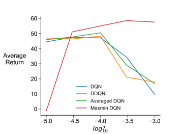
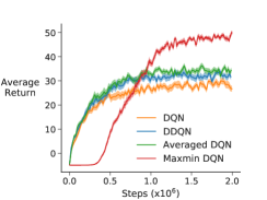
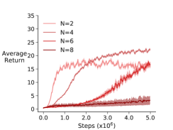
We see from Figure 4 that Maxmin DQN performs as well as or better than other algorithms. In environments where final performance is noticeably better—-Pixelcopter, Lunarlander and Asterix—the initial learning is slower. A possible explanation for this is that the Maxmin agent more extensively explored early on, promoting better final performance. We additionally show on Pixelcopter and Asterix that for smaller , Maxmin DQN learns faster but reaches suboptimal performance—behaving more like Q-learning—and for larger learns more slowly but reaches better final performance.


6 Convergence Analysis of Maxmin Q-learning
In this section, we show Maxmin Q-learning is convergent in the tabular setting. We do so by providing a more general result for what we call Generalized Q-learning: Q-learning where the bootstrap target uses a function of action values. The main condition on is that it maintains relative maximum values, as stated in Assumption 1. We use this more general result to prove Maxmin Q-learning is convergent, and then discuss how it provides convergence results for Q-learning, Ensemble Q-learning, Averaged Q-learning and Historical Best Q-learning as special cases.
Many variants of Q-learning have been proposed, including Double Q-learning (van Hasselt, 2010), Weighted Double Q-learning (Zhang et al., 2017), Ensemble Q-learning (Anschel et al., 2017), Averaged Q-learning (Anschel et al., 2017), and Historical Best Q-learning (Yu et al., 2018). These algorithms differ in their estimate of the one-step bootstrap target. To encompass all variants, the target action-value of Generalized Q-learning is defined based on action-value estimates from both dimensions:
| (2) |
where is the current time step and the action-value function is a function of :
| (3) |
For simplicity, the vector is denoted as , same for . The corresponding update rule is
| (4) |
For different functions, Generalized Q-learning reduces to different variants of Q-learning, including Q-learning itself. For example, Generalized Q-learning can be reduced to Q-learning simply by setting , with . Double Q-learning can be specified with , , and .
We first introduce Assumption 1 for function in Generalized Q-learning, and then state the theorem. The proof can be found in Appendix B.
Assumption 1 (Conditions on )
Let and where , and , and .
-
(i)
If , , , and , then .
-
(ii)
, .
We can verify that Assumption 1 holds for Maxmin Q-learning. Set and set to be a positive integer. Let and define . It is easy to check that part (i) of Assumption 1 is satisfied. Part (ii) is also satisfied because
Assumption 2 (Conditions on the step-sizes)
There exists some (deterministic) constant such that for every , , and with probability ,
Theorem 2
Assume a finite MDP and that Assumption 1 and 2 hold. Then the action-value functions in Generalized Q-learning, using the tabular update in Equation (3), will converge to the optimal action-value function with probability , in either of the following cases: (i) , or (ii) , where is an absorbing state and all policies are proper.
As shown above, because the function for Maxmin Q-learning satisfies Assumption 1, then by Theorem 2 it converges. Next, we apply Theorem 2 to Q-learning and its variants, proving the convergence of these algorithms in the tabular case. For Q-learning, set and . Let . It is straightforward to check that Assumption 1 holds for function . For Ensemble Q-learning, set and set to be a positive integer. Let . Easy to check that Assumption 1 is satisfied. For Averaged Q-learning, the proof is similar to Ensemble Q-learning except that and is a positive integer. For Historical Best Q-learning, set and to be a positive integer. We assume that all auxiliary action-value functions are selected from action-value functions at most updates ago. Define to be the largest action-value among for state . Assumption 1 is satisfied and the convergence is guaranteed.
7 Conclusion
Overestimation bias is a byproduct of Q-learning, stemming from the selection of a maximal value to estimate the expected maximal value. In practice, overestimation bias leads to poor performance in a variety of settings. Though multiple Q-learning variants have been proposed, Maxmin Q-learning is the first solution that allows for a flexible control of bias, allowing for overestimation or underestimation determined by the choice of and the environment. We showed theoretically that we can decrease the estimation bias and the estimation variance by choosing an appropriate number of action-value functions. We empirically showed that advantages of Maxmin Q-learning, both on toy problems where we investigated the effect of reward noise and on several benchmark environments. Finally, we introduced a new Generalized Q-learning framework which we used to prove the convergence of Maxmin Q-learning as well as several other Q-learning variants that use action-value estimates.
Acknowledgments
We would like to thank Huizhen Yu and Yi Wan for their valuable feedback and helpful discussion.
References
- Anschel et al. (2017) Oron Anschel, Nir Baram, and Nahum Shimkin. Averaged-DQN: Variance Reduction and Stabilization for Deep Reinforcement Learning. In International Conference on Machine Learning, pp. 176–185, 2017.
- Bertsekas & Tsitsiklis (1989) Dimitri P Bertsekas and John N Tsitsiklis. Parallel and Distributed Computation: Numerical Methods, volume 23. Prentice hall Englewood Cliffs, NJ, 1989.
- Bertsekas & Tsitsiklis (1996) Dimitri P Bertsekas and John N Tsitsiklis. Neuro-dynamic Programming, volume 5. Athena Scientific Belmont, MA, 1996.
- Brockman et al. (2016) Greg Brockman, Vicki Cheung, Ludwig Pettersson, Jonas Schneider, John Schulman, Jie Tang, and Wojciech Zaremba. OpenAI Gym. arXiv preprint arXiv:1606.01540, 2016.
- David & Nagaraja (2004) Herbert Aron David and Haikady Navada Nagaraja. Order Statistics. Encyclopedia of Statistical Sciences, 2004.
- Fujimoto et al. (2018) Scott Fujimoto, Herke Hoof, and David Meger. Addressing function approximation error in actor-critic methods. In International Conference on Machine Learning, pp. 1587–1596, 2018.
- Haarnoja et al. (2018) Tuomas Haarnoja, Aurick Zhou, Pieter Abbeel, and Sergey Levine. Soft actor-critic: Off-policy maximum entropy deep reinforcement learning with a stochastic actor. In International Conference on Machine Learning, pp. 1861–1870, 2018.
- Hado van Hasselt et al. (2016) Hado Hado van Hasselt, Arthur Guez, and David Silver. Deep Reinforcement Learning with Double Q-learning. In AAAI Conference on Artificial Intelligence, 2016.
- Lee et al. (2013) Donghun Lee, Boris Defourny, and Warren B. Powell. Bias-corrected Q-learning to Control Max-operator Bias in Q-learning. In IEEE Symposium on Adaptive Dynamic Programming and Reinforcement Learning, pp. 93–99, 2013.
- Melo & Ribeiro (2007) Francisco S Melo and M Isabel Ribeiro. Q-learning with Linear Function Approximation. In International Conference on Computational Learning Theory, pp. 308–322, 2007.
- Strehl et al. (2009) Alexander L. Strehl, Lihong Li, and Michael L. Littman. Reinforcement Learning in Finite MDPs: PAC Analysis. Journal of Machine Learning Research, 10(Nov):2413–2444, 2009.
- Sutton & Barto (2018) Richard S Sutton and Andrew G Barto. Reinforcement Learning: An Introduction. MIT Press, second edition, 2018.
- Szita & Lőrincz (2008) István Szita and András Lőrincz. The Many Faces of Optimism: A Unifying Approach. In International Conference on Machine learning, pp. 1048–1055. ACM, 2008.
- Tasfi (2016) Norman Tasfi. Pygame learning environment. https://github.com/ntasfi/PyGame-Learning-Environment, 2016.
- Thrun & Schwartz (1993) Sebastian Thrun and Anton Schwartz. Issues in Using Function Approximation for Reinforcement Learning. In Fourth Connectionist Models Summer School, 1993.
- Tsitsiklis (1994) John N Tsitsiklis. Asynchronous Stochastic Approximation and Q-learning. Machine learning, 1994.
- van Hasselt (2010) Hado van Hasselt. Double Q-learning. In Advances in Neural Information Processing Systems, pp. 2613–2621, 2010.
- Watkins (1989) Chris Watkins. Learning from Delayed Rewards. PhD thesis, King’s College, Cambridge, 1989.
- Young & Tian (2019) Kenny Young and Tian Tian. MinAtar: An Atari-inspired Testbed for More Efficient Reinforcement Learning Experiments. arXiv preprint arXiv:1903.03176, 2019.
- Yu et al. (2018) Wenwu Yu, Rui Wang, Ruiying Li, Jing Gao, and Xiaohui Hu. Historical Best Q-Networks for Deep Reinforcement Learning. In International Conference on Tools with Artificial Intelligence, pp. 6–11, 2018.
- Zhang et al. (2017) Zongzhang Zhang, Zhiyuan Pan, and Mykel J. Kochenderfer. Weighted Double Q-learning. In International Joint Conference on Artificial Intelligence, pp. 3455–3461, 2017.
Appendix A The Proof of Theorem 1
We first present Lemma 1 here as a tool to prove Theorem 1. Note that the first three properties in this lemma are well-known results of order statistics (David & Nagaraja, 2004).
Lemma 1
Let be i.i.d. random variables from an absolutely continuous distribution with probability density function(PDF) and cumulative distribution function (CDF) . Denote and . Set and . Denote the PDF and CDF of as and , respectively. Similarly, denote the PDF and CDF of as and , respectively. We then have
-
(i)
and .
-
(ii)
. .
-
(iii)
. .
-
(iv)
If , we have and for any positive integer .
Proof.
-
(i)
By the definition of , we have . Thus . Since , . The proof of can be found in (David & Nagaraja, 2004, Chapter 4 Section 4.2).
-
(ii)
We first consider the cdf of . . Then the pdf of is .
-
(iii)
Similar to (ii), we first consider cdf of . . Then the pdf of is .
-
(iv)
Since , we have and . . It is easy to check that for any positive integer .
Next, we prove Theorem 1.
Proof. Let and be the cdf and pdf of , respectively. Similarly, Let and be the cdf and pdf of . Since is sampled from , it is easy to get and . By Lemma 1, we have and . The expectation of is
Let , so that . Substitute by where , then
Each term in the denominator decreases as increases, because gets smaller. Therefore, and . Using this, we conclude that decreases as increases and and .
By Lemma 1, the variance of is
decreases as increases. In particular, for and for .
The bias-variance trade-off of Maxmin Q-learning is illustrated by the empirical results in Figure 5, which support Theorem 1. For each , can be selected such that the absolute value of the expected estimation bias is close to according to Theorem 1. As increases, we can adjust to reduce both the estimation variance and the estimation bias.


Finally, we prove the result of the Corollary.
Corollary 1 Assuming the samples are evenly allocated amongst the estimators, then where is the variance of samples for and, for the estimator that uses all samples for a single estimate,
Under this uniform random noise assumption, for , .
Proof. Because is a sample mean, its variance is where is the variance of samples for and its mean is (because it is an unbiased sample average). Consequently, has mean zero and variance . Because is a uniform random variable which has variance , we know that . Plugging this value into the variance formula in Theorem 1, we get that
because for the sample average that uses all the samples for one estimator. Easy to verify that for , .
Appendix B The Convergence Proof of Generalized Q-learning
The convergence proof of Generalized Q-learning is based on Tsitsiklis (1994). The key steps to use this result for Generalized Q-learning include showing that the operator is a contraction and verifying the noise conditions. We first show these two steps in Lemma 2 and Lemma 3. We then use these lemmas to make the standard argument for convergence.
B.1 Problem Setting for Generalized Q-learning
Consider a Markov decision problem defined on a finite state space . For every state , there is a finite set of possible actions for state and a set of non-negative scalars , , , such that for all . The scalar is interpreted as the probability of a transition to , given that the current state is and action is applied. Furthermore, for every state and action , there is a random variable which represents the reward if action is applied at state . We assume that the variance of is finite for every and .
A stationary policy is a function defined on such that for all . Given a stationary policy, we obtain a discrete-time Markov chain with transition probabilities
| (5) |
Let be a discount factor. For any stationary policy and initial state , the state value is defined by
| (6) |
The optimal state value function is defined by
| (7) |
The Markov decision problem is to evaluate the function . Once this is done, an optimal policy is easily determined.
Markov decision problems are easiest when the discount is strictly smaller than . For the undiscounted case (), we will assume throughout that there is a reward-free state, say state , which is absorbing; that is, and for all . The objective is then to reach that state at maximum expected reward. We say that a stationary policy is proper if the probability of being at the absorbing state converges to as time converges to infinity; otherwise, we say that the policy is improper.
We define the dynamic programming operator , with components , by letting
| (8) |
It is well known that if , then is a contraction with respect to the norm and is its unique fixed point.
For Generalized Q-learning algorithm, assume that there are estimators of action-values . Let be the cardinality of and be the cardinality of . We use a discrete index variable in order to count iterations. Denote . After iterations, we have a vector and , with components , , , and .
By definition, for , we have
| (9) |
For , we have . And we update according to the formula
| (10) |
where
| (11) |
Here, each is a nonnegative step-size coefficient which is set to zero for those and for which is not to be updated at the current iteration. Furthermore, is a random sample of the immediate reward if action is applied at state . is a random successor state which is equal to with probability . Finally, is defined as
| (12) |
where is a mapping from to . It is understood that all random samples that are drawn in the course of the algorithm are drawn independently.
Since for , we just preserve current available action-values, we only focus on the case that in the sequel. Let be the mapping from into with components defined by
| (13) |
and note that
| (14) |
If , we can do more updates such that , , , and .
B.2 Key Lemmas and the Proofs
Lemma 2
Assume Assumption 1 holds for function in Generalized Q-learning. Then we have
Proof. Under Assumption 1, the conditional variance of given , is bounded above by the largest possible value that this random variable could take, which is . We then take the conditional variance of both sides of Equation 16, to obtain
| (17) |
We have assumed here that is independent from . If it is not, the right-hand side in the last inequality must be multiplied by , but the conclusion does not change.
Lemma 3
is a contraction mapping, in each of the following cases:
-
(i)
.
-
(ii)
and where is an absorbing state. All policies are proper.
Proof. For discounted problems (), Equation 13 easily yields ,
| (18) |
In particular, is a contraction mapping, with respect to the maximum norm .
For undiscounted problems (), our assumptions on the absorbing state imply that the update equation for degenerates to , for all . We will be assuming in the sequel, that is initialized at zero. This leads to an equivalent description of the algorithm in which the mappings of Equation 13 are replaced by mappings satisfying if and for all , and .
Let us consider the special case where every policy is proper. By Proposition 2.2 in the work of (Bertsekas & Tsitsiklis, 1996), there exists a vector such that is a contraction with respect to the norm . In fact, a close examination of the proof of this Proposition 2.2 shows that this proof is easily extended to show that the mapping (with components ) is a contraction with respect to the norm , where for every and .
B.3 Models and Assumptions
In this section, we describe the algorithmic model to be employed and state some assumptions that will be imposed.
The algorithm consists of noisy updates of a vector , for the purpose of solving a system of equations of the form . Here is assumed to be a mapping from into itself. Let : be the corresponding component mappings; that is, for all .
Let be the set of non-negative integers. We employ a discrete ”time” variable , taking values in . This variable need not have any relation with real time; rather, it is used to index successive updates. Let be the value of the vector at time and let denote its th component. Let be an infinite subset of indicating the set of times at which an update of is performed. We assume that
| (19) |
Regarding the times that is updated, we postulate an update equation of the form
| (20) |
Here, is a step-size parameter belonging to , is a noise term, and is a vector of possibly outdated components of . In particular, we assume that
| (21) |
where each is an integer satisfying . If no information is outdated, we have and for all ; the reader may wish to think primarily of this case. For an interpretation of the general case, see (Bertsekas & Tsitsiklis, 1989). In order to bring Eqs. 19 and 20 into a unified form, it is convenient to assume that , and are defined for every , , and , but that and for .
We will now continue with our assumptions. All variables introduced so far are viewed as random variables defined on a probability space and the assumptions deal primarily with the dependencies between these random variables. Our assumptions also involve an increasing sequence of subfields of . Intuitively, is meant to represent the history of the algorithm up to, and including the point at which the step-sizes for the th iteration are selected, but just before the noise term is generated. Also, the measure-theoretic terminology that ”a random variable is -measurable” has the intuitive meaning that is completely determined by the history represented by .
The first assumption, which is the same as the total asynchronism assumption of Bertsekas & Tsitsiklis (1989), guarantees that even though information can be outdated, any old information is eventually discarded.
Assumption 3
For any and , , with probability 1.
Our next assumption refers to the statistics of the random variables involved in the algorithm.
Assumption 4
Let be an increasing sequence of subfields of .
-
(i)
is -measurable.
-
(ii)
For every and is -measurable.
-
(iii)
For every , and , and are -measurable.
-
(iv)
For every and , we have .
-
(v)
There exist (deterministic) constants and such that
(22)
Assumption 4 allows for the possibility of deciding whether to update a particular component at time , based on the past history of the process. In this case, the step-size becomes a random variable. However, part of the assumption requires that the choice of the components to be updated must be made without anticipatory knowledge of the noise variables that have not yet been realized.
Finally, we introduce a few alternative assumptions on the structure of the iteration mapping . We first need some notation: if , the inequality is to be interpreted as for all . Furthermore, for any positive vector , we define a norm on by letting
| (23) |
Notice that in the special case where all components of are equal to , is the same as the maximum norm .
Assumption 5
Let .
-
(i)
The mapping is monotone; that is, if , then .
-
(ii)
The mapping is continuous.
-
(iii)
The mapping has a unique fixed point .
-
(iv)
If is the vector with all components equal to , and is a positive scalar, then
(24)
Assumption 6
There exists a vector , a positive vector , and a scalar , such that
| (25) |
Assumption 7
There exists a positive vector , a scalar , and a scalar such that
| (26) |
Assumption 8
There exists at least one proper stationary policy. Every improper stationary policy yields infinite expected cost for at least one initial state.
Theorem 4
B.4 Proof of Theorem 2
We first state Theorem 2 here again and then show the proof.
Theorem 2
Assume a finite MDP and that Assumption 1 and 2 hold. Then the action-value functions in Generalized Q-learning, using tabular update in Equation (3), will converge to the optimal action-value function with probability , in each of the following cases:
-
(i)
.
-
(ii)
and where is an absorbing state. All policies are proper.
Proof. We first check Assumptions 3, 4, 2, and 6 in Section B.3 are satisfied. Then we simply apply Theorem 5 to Generalized Q-learning.
Assumption 3 is satisfied in the special case where , which is what was implicitly assumed in Equation 10, but can be also satisfied even if we allow for outdated information.
Regarding Assumption 4, parts and of the assumption are then automatically valid. Part is quite natural: in particular, it assumes that the required samples are generated after we decide which components to update during the current iteration. Part is automatic from Equation 16. Part is satisfied by Lemma 2.
Assumption 2 needs to be imposed on the step-sizes employed by the Generalized Q-learning algorithm. This assumption is standard for stochastic approximation algorithms. In particular, it requires that every state-action pair is simulated an infinite number of times.
Appendix C Additional Empirical Results
C.1 MDP results
Comparison of three algorithms using the simple MDP in Figure 1 with different values of is shown in Figure 6. For , the learning curves of action value are shown in . Here, the true action value is . For , the learning curves of action value are shown in . The true action value is . All results were averaged over runs.


C.2 Mountain Car results


Comparison of four algorithms on Mountain Car under different reward settings is shown in Figure 7. All experimental results were averaged over runs. Note that for reward variance , both Q-learning and Averaged Q-learning fail to reach the goal position in steps so there are no learning curves shown in Figure for these two algorithms.
C.3 Benchmark Environment results
The sensitivity analysis results of seven benchmark environment are shown in Figure 8.