Maximum-Likelihood-Estimate Hamiltonian learning via efficient and robust quantum likelihood gradient

Understanding the quantum states and the corresponding properties of a given quantum Hamiltonian is a crucial problem in quantum physics. Many powerful numerical and theoretical tools have been developed for such purposes and made compelling progress [1, 2, 3, 4, 5]. On the other hand, with the rapid experimental developments of quantum technology, e.g., near-term quantum computation [6, 7] and simulation [8, 9, 10, 11, 12, 13, 14], it is also vital to explore the inverse problem, e.g., Hamiltonian learning - optimize a model Hamiltonian characterizing a quantum system with respect to the measurement results. Given the knowledge and assumption of a target system, researchers have achieved many resounding successes modeling quantum Hamiltonians with physical pictures and phenomenological approaches [15, 16]. However, such subjective perspectives may risk biases and are commonly insufficient on detailed quantum devices. Therefore, the explorations for objective Hamiltonian learning strategies have attracted much recent attention [17, 18, 19, 20, 21, 22, 23, 24, 25].

There are mainly two categories of Hamiltonian-learning strategies, based upon either quantum measurements on a large number of (identical copies of) quantum states, e.g., Gibbs states or eigenstates [17, 18, 19, 20, 21, 22], or initial states’ time evolution dynamics [23, 24, 25, 26], corresponding to the target quantum system. For example, given the measurements of the correlations of a set of local operators, the kernel of the resulting correlation matrix offers a candidate model Hamiltonian [17, 18, 19]. On the other hand, while established theoretically, most approaches suffer from elevated costs and are limited to small systems in experiments or numerical simulations [19, 20, 27, 28]. Besides, there remains much room for improvements in stability towards noises and temperature ranges.

Maximum likelihood estimation (MLE) is a powerful tool that parameterizes and then optimizes the probability distribution of a statistical model so that the given observed data is most probable. MLE’s intuitive and flexible logic makes it a prevailing method for statistical inference. Adding to its wide range of applications, MLE has been applied successfully to quantum state tomography[29, 30, 31, 32, 33], providing the most probable quantum states given the measurement outputs.

Inspired by MLE’s successes in quantum problems, we propose a general MLE Hamiltonian learning protocol: given finite-temperature measurements of the target quantum system in thermal equilibrium, we optimize the model Hamiltonian towards the MLE step-by-step via a “quantum likelihood gradient”. We show that such quantum likelihood gradient, acting collectively on all presenting operators, is negative semi-definite with respect to the negative-log-likelihood function and thus provides efficient optimization. In addition, our strategy may take advantage of the locality of the quantum system, therefore allowing us to extend studies to larger quantum systems with tailored quantum many-body ansatzes such as Lanczos, quantum Monte Carlo (QMC), density matrix renormalization group (DMRG), and finite temperature tensor network (FTTN) [34, 35] algorithms in suitable scenarios. We also demonstrate that MLE Hamiltonian learning is more accurate, less restrictive, and more robust against noises and broader temperature ranges. Further, we generalize our protocol to measurements on pure states, such as the target quantum systems’ ground states or quantum chaotic eigenstates. Therefore, MLE Hamiltonian learning enriches our arsenal for cutting-edge research and applications of quantum devices and experiments, such as quantum computation, quantum simulation, and quantum Boltzmann machines [36].

We organize the rest of the paper as follows: In Sec. II, we review the MLE context and introduce the MLE Hamiltonian learning protocol; especially, we show explicitly that the corresponding quantum likelihood gradient leads to a negative semi-definite change to the negative-log-likelihood function. Via various examples in Sec. III, we demonstrate our protocol’s capability, especially its robustness against noises and temperature ranges. We generalize the protocol to quantum measurements of pure states in Sec. IV and Appendix D, with consistent results for exotic quantum systems such as quantum critical and topological models. We summarize our studies in Sec. V with a conclusion on our protocol’s advantages (and limitations), potential applications, and future outlooks.

To start, we consider an unknown target quantum system $\hat{H}_{s}=\sum_{j}\mu_{j}\hat{O}_{j}$ in thermal equilibrium, and measurements of a set of observables $\{\hat{O}_{i}\}$ on its Gibbs state $\hat{\rho}_{s}=\exp(-\beta\hat{H}_{s})/\mbox{tr}[\exp(-\beta\hat{H}_{s})]$, where $\beta$ is the inverse temperature. Given a sufficient number $N_{i}$ of measurements of the operator $\hat{O}_{i}$, the occurrence time $f_{\lambda_{i}}$ of the $\lambda_{i}^{th}$ eigenvalue $o_{\lambda_{i}}$ approaches:

where $p_{\lambda_{i}}=f_{\lambda_{i}}/N_{i}$ denotes the statistics of the outcome $o_{\lambda_{i}}$, and $\hat{P}_{\lambda_{i}}$ is the corresponding projection operator to the $o_{\lambda_{i}}$ sector. Our goal is to locate the model Hamiltonian $\hat{H}_{s}$ for the quantum system, which commonly requires the presence of all $\hat{H}_{s}$’s terms in the measurement set $\{\hat{O}_{i}\}$.

Following previous MLE analysis [29, 30, 31, 32, 33], the statistical weight of any given state $\hat{\rho}$ is:

upto a trivial factor, where $N_{tot}=\sum_{i}N_{i}$ is the total number of measurements. For Hamiltonian learning, we search for (the set of parameters ${\mu_{j}}$ of) the MLE Hamiltonian $\hat{H}$, whose Gibbs state $\hat{\rho}$ maximizes the likelihood function in Eq. 2. The maximum condition for Eq. 2 can be re-expressed as:

see Appendix A for a detailed review. Solving Eq. 3 is a nonlinear and nontrivial problem, for which many algorithms have been proposed [31, 30, 32, 33]. For example, we can employ iterative updates $\hat{\rho}_{k+1}\propto\hat{R}(\hat{\rho}_{k})\hat{\rho}_{k}\hat{R}(\hat{\rho}_{k})$ until Eq. 3 is fulfilled [31]. These algorithms mostly center around the parameterization and optimization of a quantum state $\hat{\rho}$, whose cost is exponential in the system size. Besides, such iterative updates do not guarantee that the quantum state $\hat{\rho}$ remains a Gibbs form, especially when the measurements are insufficient to uniquely determine the state (e.g., large noises or small numbers of measurements and there are many quantum states satisfying Eq. 3). Consequently, extracting $\hat{H}\propto-\frac{1}{\beta}\ln\hat{\rho}$ from $\hat{\rho}$ further adds up to the inconvenience.

Considering that the operator $\hat{R}(\hat{\rho})$ has the same operator structure as the Hamiltonian, we take an alternative stance for the Hamiltonian learning task and update the candidate Hamiltonian $\hat{H}_{k}$, i.e., the model parameters, collectively and iteratively. In particular, we integrate the corrections to the Hamiltonian coefficients to the operator $\hat{R}(\hat{\rho})$, which offers such a quantum likelihood gradient (Fig. 1):

where $\gamma>0$ is the learning rate - a small parameter controlling the step size. We denote $\hat{R}_{k}\equiv\hat{R}(\hat{\rho}_{k})$ for short here afterwards. Compared with previous Hamiltonian extractions from MLE quantum state tomography, the update in Eq. 4 possesses several advantages in Hamiltonian learning. First, we can utilize the Hamiltonian structure (e.g., locality) to choose suitable numerical tools (e.g., QMC and FTTN) and even calculate within the subregions - we circumvent the costly parametrization of the quantum state $\hat{\rho}$. Also, the update guarantees a state in its Gibbs form. Last but not least, we will show that for $\gamma\ll 1$, such a quantum likelihood gradient in Eq. 4 yields a negative semi-definite contribution to the negative-log-likelihood function, guaranteeing the MLE Hamiltonian (upto a trivial constant) at its convergence and an efficient optimization toward it.

Theorem: For $\gamma\ll 1$, $\gamma>0$, the quantum likelihood gradient in Eq. 4 yields a negative semi-definite contribution to the negative-log-likelihood function $M(\hat{\rho}_{k+1})=-\frac{1}{N_{tot}}\log\mathcal{L}(\hat{\rho}_{k+1})$.

Proof: We note that upto linear order in $\gamma\ll 1$:

where ${\rm ad}_{\hat{A}}^{j}\hat{B}=[\hat{A},{\rm ad}_{\hat{A}}^{j-1}\hat{B}]$ and ${\rm ad}_{\hat{A}}^{0}\hat{B}=\hat{B}$ are the adjoint action of the Lie algebra. The first and third lines are based on the Zassenhaus formula[37] and the Baker-Hausdorff formula [37], respectively, while the second line neglects terms above the linear order of $\gamma$.

Following this, we can re-express the quantum state in Eq. 4 as:

where we have used $\mbox{tr}[\hat{\rho}_{k}\hat{R}_{k}]=1$ as a direct consequence of $R_{k}$’s definition in Eq. 3.

Subsequently, after introducing the quantum likelihood gradient, the negative-log-likelihood function becomes:

where we keep terms upto linear order of $\gamma$ in the $\log$ expansion.

On the other hand, we can establish the following inequality:

where $Z_{k}=\mbox{tr}[e^{-\beta\hat{H}_{k}}]$ is the partition function, $||A||_{F}=\sqrt{\mbox{tr}[A^{\dagger}A]}$ is the Frobenius norm of matrix $A$, and the non-negative definiteness of $\hat{\rho}_{k}$ allows $\hat{\rho}_{k}=(\hat{\rho}_{k}^{1/2})^{2}=(e^{-\beta\hat{H}_{k}/2})^{2}/Z_{k}$. The inequality in the fourth line follows the Cauchy-Schwarz inequality.

We note that the equality - the convergence criteria of our MLE Hamiltonian learning protocol - is established if and only if:

which implies the conventional MLE optimization target $\hat{R}\hat{\rho}=\hat{\rho}$ in Eq. 3. We can also establish such consistency from our iterative convergence ¹¹1In practice, given sufficient measurements, we have $\hat{R}_{k}\sim\hat{I}$ dictating the quantum likelihood gradient at the iteration’s convergence. following Eq. 4:

where we have used the commutation relation $[\hat{R}_{k},\hat{H}_{k}]=0$ between the Hermitian operators $\hat{R}_{k}$ and $\hat{H}_{k}$ following $[\hat{R}_{k},\hat{\rho}_{k}]=[\hat{R}_{k},e^{-\beta\hat{H}_{k}}]=0$.

Finally, combining Eq. 7 and Eq. 8, we have shown that $M(\hat{\rho}_{k+1})-M(\hat{\rho}_{k})\leq 0$ is a negative semi-definite quantity, which proves the theorem.

We conclude that the quantum likelihood gradient in Eq. 4 offers an efficient and collective optimization towards the MLE Hamiltonian, modifying all model parameters simultaneously. For each step of quantum likelihood gradient, the most costly calculation is on $\hat{\rho}_{k+1}$, or more precisely, the expectation value $\mbox{tr}[\hat{\rho}_{k+1}\hat{P}_{\lambda_{i}}]$ from $\hat{H}_{k+1}$. Fortunately, this is a routine calculation in quantum many-body physics and condensed matter physics with various tailored candidate algorithms under different scenarios. For example, we may resort to the FTTN, or the QMC approaches, which readily apply to much larger systems than brute-force exact diagonalization. Thus, we emphasize that MLE Hamiltonian learning works with evaluations of the expectation values of quantum states instead of the more expensive quantum states themselves in their entirety.

Interestingly, MLE Hamiltonian learning also allows a more local stance. For a given Hamiltonian, the necessary expectation value of its Gibbs state $\mbox{tr}[\hat{\rho}\hat{P}_{\lambda_{i}}]$ takes the form:

where $\hat{\rho}^{A}_{eff}$ is the reduced density operator defined upon a relatively local subsystem $A$ still containing $\hat{P}_{\lambda_{i}}$. The effective Hamiltonian $\hat{H}_{eff}^{A}=\hat{H}_{A}+\hat{V}_{eff}^{A}$ of the subregion $A$ contains the existing terms $\hat{H}_{A}$ within the subsystem and the effective interacting terms $\hat{V}_{eff}^{A}$ from the trace operation [39]. According to the conclusions of the quantum belief propagation theory [40, 39], the locality of the interaction in the latter term $||\hat{V}_{eff}^{A}(l_{A})||_{F}\propto(\beta/\beta_{c})^{l_{A}/r}$, where $\beta$ ($\beta_{c}$) denotes the current (model-dependent critical) inverse temperature, $l_{A}$ is the distance between a specific site in the bulk of $A$ and the boundary of the subregion $A$, and $r$ is the maximum acting distance(diameter) of a single operator in the original Hamiltonian(similar to the k-local in the next section). Thus, when $\beta<\beta_{c}$(especially when $\beta\ll\beta_{c}$), $\hat{V}_{eff}^{A}$ is exponentially localized around the boundary of $A$, and the effective Hamiltonian in the bulk of $A$ remains the same as that of the original $\hat{H}_{A}$ of the entire system. Therefore, we may further boost the efficiency of MLE Hamiltonian learning by redirecting the expectation-value evaluations of the global quantum system to that of a series of local patches, as we will show in the next section.

In summary, given the quantum measurements of a thermal (Gibbs) state: $\{\hat{O}_{i}\}$, $N_{i}$, and $f_{\lambda_{i}}$, we can perform MLE Hamiltonian learning to obtain the MLE Hamiltonian via the following steps (Fig. 1):

• 1)

  Initialization/Update:

  For initialization, start with a random model Hamiltonian $\hat{H}_{0}$:

  $$\hat{H}_{0}=\sum_{i}\mu_{i}\hat{O}_{i},$$

  (12)

  or an identity Hamiltonian.

  For update, carry out the quantum likelihood gradient:

  $$\hat{H}_{k+1}=\hat{H}_{k}-\gamma\hat{R}_{k},$$

  (13)

  where $\hat{R}_{k}$ is defined in Eq. 3 or Eq. 16.

• 2)

  Evaluate the properties $\mbox{tr}[\hat{\rho}_{k}\hat{P}_{\lambda_{i}}]$ of the quantum state:

  $$\hat{\rho}_{k}=\frac{e^{-\beta\hat{H}_{k}}}{\mbox{tr}[e^{-\beta\hat{H}_{k}}]},$$

  (14)

  with suitable numerical methods.

• 3)

  Check for convergence: loop back to step 1) to update, $k\rightarrow k+1$, if the relative entropy $M(\hat{\rho}_{k})-M_{0}\geq\epsilon$ is above a given threshold $\epsilon$; otherwise, terminate the process, and the final $\hat{H}_{k}$ is the result for the MLE Hamiltonian. Here, $M_{0}$ is the theoretical minimum of the negative-log-likelihood function:

  $$M_{0}=-\sum_{i,\lambda_{i}}\frac{N_{i}}{N_{tot}}p_{\lambda_{i}}\log{p_{\lambda_{i}}}.$$

  (15)

In practice, $\hat{R}_{k}$ in Eq. 4 is singular for small values of $\mbox{tr}[\hat{\rho}_{k}\hat{P}_{\lambda_{i}}]$ and may become numerically unstable, which requires a minimal or dynamical learning rate $\gamma$ to maintain the range of quantum likelihood gradient properly. Instead, we may employ a re-scaled version of $\hat{R}_{k}$:

where $f_{g}$ is a monotonic tuning-function:

which maps its argument in $(0,\infty)$ to a finite range $(0,g)$. Such a re-scaled $\tilde{\hat{R}}_{k}$ regularizes the quantum likelihood gradient and allows a simple yet relatively larger learning rate $\gamma$ for more efficient MLE Hamiltonian learning. We also have $f_{g}(1)=1$, therefore $\tilde{\hat{R}}_{k}\rightarrow\hat{R}_{k}$ as we approach convergence. We will mainly employ $\tilde{\hat{R}}_{k}$ for our examples in the following sections.

In addition to the negative-log-likelihood function $M(\hat{\rho}_{k})$, we also consider the Hamiltonian distance as another criterion on the quality of Hamiltonian learning:

where $\vec{\mu}_{s}$ and $\vec{\mu}_{k}$ are the (vectors of) coefficients ²²2We typically perform MLE Hamiltonian learning and update the model Hamiltonian on the projection-operator basis; therefore, we transform the Hamiltonian back to the original, ordinary operator basis before $\Delta\vec{\mu}_{k}$ evaluations. of the target Hamiltonian and the learned Hamiltonian after $k$ iterations, respectively. However, we do not recommend $\Delta{\vec{\mu}}_{k}$($\Delta\mu$ for short) as convergence criteria as $\vec{\mu}_{s}$ is generally unknown aside from benchmark scenarios [28].

In this section, we demonstrate the performance of the MLE Hamiltonian learning protocol. For better numerical simulations, we consider the $k$-local Hamiltonians, with operators acting non-trivially on no more than $k$ contiguous sites in each direction. For example, for a 1-dimensional spin-$\frac{1}{2}$ system, a $k$-local operator for $k=2$ takes the form $\hat{S}_{i}^{\alpha}\hat{S}_{i+1}^{\beta}$ or $\hat{S}_{i}^{\alpha}$, $\alpha,\beta\in\{x,y,z\}$, where $\hat{S}_{i}^{\alpha}$ denotes the spin operator. In particular, we focus on general 1D quantum spin chains with $k=2$, taking the following form:

where $\hat{S}_{i}^{\alpha}$ denotes the spin operator on site $i$, $\alpha,\beta,\in\{x,y,z\}$. There are $12L-9$ 2-local operators under the open boundary condition, where $L$ is the system size. We generate the model parameters $\vec{\mu}_{s}=\{J_{i}^{\alpha\beta},h_{i}^{\alpha}\}$ randomly following a uniform distribution in $[-1,1]$. This Hamiltonian $\hat{H}_{s}$, specifically the model parameters $\vec{\mu}_{s}$, will be our target for MLE Hamiltonian learning. As the protocol’s inputs, we simulate quantum measurements of all 2-local operators $\{\hat{O}_{i}\}$ on the Gibbs states of $\hat{H}_{s}$ numerically via exact diagonalization on small systems and FTTN for large systems. For the latter, we use a tensor network ansatz called the “ancilla” method [34], where we purify a Gibbs state with some auxiliary qubits $\hat{\rho}_{s}=\mbox{tr}_{aux}|\psi_{s}\rangle\langle\psi_{s}|$, and obtain $\ket{\psi_{s}}=e^{-\beta\hat{H}_{s}/2}\ket{\psi_{0}}$ from a maximally-entangled state $\ket{\psi_{0}}$ via imaginary time evolution. In addition, given a large number $n$ of Trotter steps, the imaginary time evolution operator $e^{-\beta\hat{H}_{s}/2}$ is decomposed into Trotter gates’ product as $(\Pi_{i}e^{-\mu_{i}\hat{O}_{i}\beta/2n})^{n}+O(\beta^{2}/n)$. Here, we set the Trotter step $\delta t=\beta/n\in[0.01,0.1]$, for which the Trotter errors of order $O(\beta^{2}/n)$ show little impact on our protocol’s accuracy. Without loss of generality, we employ the integrated FTTN algorithm in the ITensor numerical toolkit [35], and set the number of measures $N_{i}=N$ for all operators in our examples for simplicity.

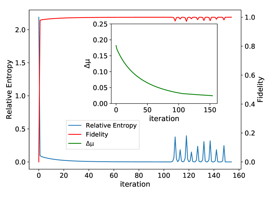
As we demonstrate in Fig. 2, MLE Hamiltonian learning obtains the target Hamiltonians with high accuracy and efficiency under various settings of system sizes and inverse temperatures $\beta$. Besides, instead of the original quantum likelihood gradient in Eq. 3, we may obtain a faster convergence with the re-scaled $\tilde{\hat{R}}_{k}$ in Eq. 16 and a larger learning rate, as we discuss in Appendix B. In the following numerical examples, we use the re-scaled quantum likelihood gradient $\tilde{\hat{R}}_{k}$ and set $g=2$ for the tuning function in Eq. 17. Within the given iterations, not only have we achieved results (Hamiltonian distance $\Delta\mu\sim O(10^{-12})$ and relative entropy $M(\hat{\rho}_{k})-M_{0}\sim O(10^{-16})$) comparable to, if not exceeding, previous methods [19] for $L=10$ systems and $\beta=1$ straightforwardly, but we have also achieved satisfactory consistency ($\Delta\mu\sim O(10^{-2})$ and $M(\hat{\rho}_{k})-M_{0}\sim O(10^{-9})$) for large systems $L=100$ and low temperatures $\beta=3$ that were previously inaccessible.

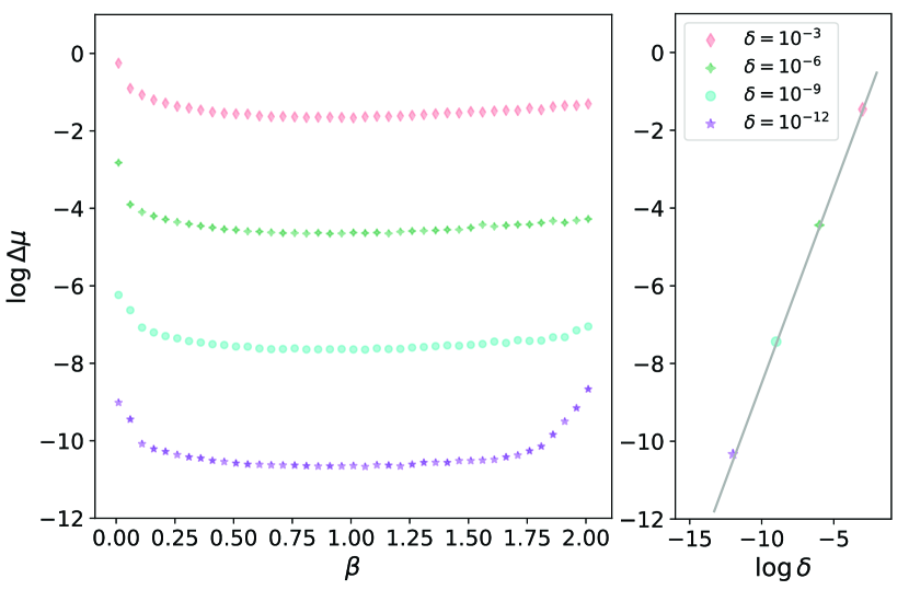
MLE Hamiltonian learning is also relatively robust against temperature and noises, two key factors impacting accuracy in Hamiltonian learning. For illustration, we include random errors $\delta\langle\hat{O}_{i}\rangle$ following Gaussian distribution with zero mean and standard deviation $\delta$ to all quantum measurements: $\langle\hat{O}_{i}\rangle\rightarrow\langle\hat{O}_{i}\rangle+\delta\langle\hat{O}_{i}\rangle$. We note that such $\delta$ may also depict the quantum fluctuations [19, 21] from a finite number of measurements $\delta\propto N_{i}^{-1/2}$. We also focus on smaller systems with $L=10$ and employ exact diagonalization to avoid confusion from potential Trotter error of the FTTN ansatz[34]. We summarize the results in Fig. 3.

Most previous algorithms on Hamiltonian learning have a rather specific applicable temperature range. For example, the high-temperature expansion of $e^{-\beta\hat{H}}$ only works in the $\beta\ll 1$ limit [42, 43]. Besides, gradient descent on the log partition function, despite a convex optimization, performs well in a narrow temperature range [20]. The gradient of this algorithm is proportional to the inverse temperature, so the algorithm’s convergence slows at high temperatures. Also, the gradient descent algorithm cannot extend to the $\beta\rightarrow\infty$ limit - the ground state, while our protocol is directly applicable to the ground states of quantum systems, as we will generalize and justify later.

MLE Hamiltonian learning is also more robust to noises, with an accuracy of Hamiltonian distance $\Delta\mu\sim O(10^{-11})$ across a broad temperature range at noise strength $\delta\sim O(10^{-12})$. Such noise level is hard to realize in practice; nevertheless, it is necessary to safeguard the correlation matrix method [17, 19, 44]. Even so, due to the uncontrollable spectral gap, the correlation matrix method is susceptible to high temperature, and its accuracy drastically decreases to $\Delta\mu\sim O(10^{-3})$ at $\beta=0.01$. In comparison, MLE Hamiltonian learning is more versatile, with an approximately linear dependence between its accuracy $\Delta\mu$ and the noise strength $\delta$ across a broad range of temperatures and noise strengths, saturating the previous bound [20]; see the right panel of Fig. 3. We also provide more detailed comparisons between the algorithms in Appendix C.

Despite efficient quantum likelihood gradient and applicable quantum many-body ansatz, the computational cost of MLE Hamiltonian learning still increases rapidly with the system size $L$. Fortunately, as stated above in Eq. 11, we may resort to calculations on local patches, especially for low dimensions and high temperatures due to their quasi-Markov property. In particular, when $\beta<\beta_{c}$ ($T>T_{c}$), the difference between the cutoff Hamiltonian $\hat{H}_{A}$ and the effective Hamiltonian $\hat{H}_{eff}^{A}$ in a local subregion $A$, $V_{eff}^{A}$, should be weak, short-ranged, and localized at $A$’s boundary [40, 39]; therefore, for those operators $\hat{P}_{\lambda_{i}}$ adequately deep inside $A$, we can use $\hat{\rho}^{A}$, the Gibbs state defined by $\hat{H}_{A}$, to estimate the corresponding $\mbox{tr}[\hat{\rho}\hat{P}_{\lambda_{i}}]$; see illustration in Fig. 4 upper panel.

For example, we apply MLE Hamiltonian learning on $L=100$ systems, where we iteratively calculate the necessary expectation values on different local patches of size $L_{A}=10,16$. We also choose different cut-offs $\Lambda$, and evaluate $\mbox{tr}[\hat{\rho}^{A}\hat{P}_{\lambda_{i}}]$ for those operators at least $\Lambda$ away from the boundaries and sufficiently deep inside the subregion $A$, so that the effective potential $V^{A}_{eff}$ may become negligible. We also employ a sufficient number of local patches to guarantee full coverage of necessary observables - operators outside $A$ or in $\Lambda_{A}$ are obtainable from another local patch $B$, as shown in the upper panel of Fig. 4, and so on so forth. Both the $L=100$ target system and the local patches for MLE Hamiltonian learning are simulated via FTTN. We have no problem achieving convergence, and the resulting Hamiltonians’ accuracy, the Hamiltonian distance $\Delta\mu$ versus the inverse temperature $\beta$, is summarized in the lower panel of Fig. 4. Indeed, the local-patch approximation is more reliable at higher temperatures, as well as with larger subsystems and cutoffs, albeit with rising costs. We also note that we can achieve much larger systems with the local patches than $L=100$ we have demonstrated.

In addition to the Gibbs states, MLE Hamiltonian learning also applies to measurements of certain eigenstates of target quantum systems:

1. The ground states are essentially the $\beta\rightarrow\infty$ limit of the Gibbs states. However, due to the order-of-limit issue, the $\gamma\rightarrow 0$ requirement of the theorem on Gibbs states forbids a direct extension to the ground states. In the Appendix D, we offer rigorous proof of the effectiveness of quantum likelihood gradient based on ground-state measurements, along with several nontrivial MLE Hamiltonian learning examples on quantum critical and topological ground states. We note that Ref. 45 offers preliminary studies on pure-state quantum state tomography, inspiring this work.

2. A highly-excited eigenstate of a (non-integrable) quantum chaotic system $\hat{H}_{s}$ is believed to obey the eigenstate thermalization hypothesis (ETH), that its density operator $\hat{\rho}_{s}=\ket{\psi_{s}}\bra{\psi_{s}}$ behaves locally indistinguishable from a Gibbs state $\hat{\rho}_{s,A}$ in thermal equilibrium [46]:

where $\beta_{s}$ is an effective temperature determined by the energy expectation value $\braket{\psi_{s}}{\hat{H}_{s}}{\psi_{s}}=\frac{\mbox{tr}[e^{-\beta_{s}\hat{H}_{s}}\hat{H}_{s}]}{\mbox{tr}[e^{-\beta_{s}\hat{H}_{s}}]}$. As MLE Hamiltonian learning only engages local operators, its applicability directly generalizes to such eigenstates $\ket{\psi_{s}}$ following ETH.

3. In general, ETH applies to eigenstates in the center of the spectrum of quantum chaotic systems, while low-lying eigenstates are too close to the ground state to exhibit ETH [47]. However, in the rest of the section, we demonstrate numerically that MLE Hamiltonian learning still works well for low-lying eigenstates.

We consider the 1D longitudinal-transverse-field Ising model [46, 47] as our target quantum system:

where the system size is $L=80$. We set $J=1$, $g_{x}=0.9045$, and $g_{z}=0.8090$. The quantum system is strongly non-integrable under such settings. Previous studies mainly focused on eigenstates in the middle of the energy spectrum. In contrast, we pick the first excited state - a typical low-lying eigenstate considered asymptotically integrable and ETH-violating [47] - for quantum measurements (via DMRG) and then MLE Hamiltonian learning for its candidate Hamiltonian (via FTTN).

We summarize the results in Fig. 5. Further, the model Hamiltonian we established is approximately equivalent to the target quantum Hamiltonian at an (inverse) temperature $\beta_{s}\approx 4$ [46], which we have absorbed into the unit of our $\hat{H}_{k}$. Therefore, we have accurately established the model Hamiltonian and derived the effective temperature consistent with previous results [46] for a low-lying excited eigenstate not necessarily following ETH. The physical reason for quantum likelihood gradient applicability in such states is an interesting problem that deserves further studies.

We have proposed a novel MLE Hamiltonian learning protocol to achieve the model Hamiltonian of the target quantum system based on quantum measurements of its Gibbs states. The protocol updates the model Hamiltonian iteratively with respect to the negative-log-likelihood function from the measurement data. We have theoretically proved the efficiency and convergence of the corresponding quantum likelihood gradient and demonstrated it numerically on multiple non-trivial examples, which show more accuracy, better robustness against noises, and less temperature dependence. Indeed, the accuracy is almost linear to the imposed noise amplitude, thus inverse proportional to the square root of the number of samples, the asymptotic upper bound[20]. Further, MLE Hamiltonian learning directly rests on the Hamiltonians and their physical properties instead of direct and costly access to the quantum many-body states. Consequently, we can resort to various quantum many-body ansatzes in our systematic quantum toolbox and even local-patch approximation when the situation allows. These advantages allow applications to larger systems and lower temperatures with better accuracy than previous approaches. On the other hand, while our protocol is generally applicable for learning any Hamiltonian, its advantages are most apparent for local Hamiltonians, where various quantum many-body ansatzes and local-patch approximation shine. Despite such limitations, we note that the physical systems are characterized by local Hamiltonians in a significant proportion of scenarios.

In addition to the Gibbs states, we have generalized the applicability of MLE Hamiltonian learning to eigenstates of the target quantum states, including ground states, ETH states, and even selected cases of low-lying excited states. We have also provided theoretical proof of quantum likelihood gradient rigor and convergence in the Appendix D, along with several other numerical examples.

Our strategy may apply to the entanglement Hamiltonians and the tomography of the quantum states under the maximum-likelihood-maximum-entropy assumption [48]. Besides, our algorithm may also provide insights into the quantum Boltzmann machine [36] - a quantum version of the classical Boltzmann machine with degrees of freedom that obey the distribution of a target quantum Gibbs state. Instead of brute-force calculations of the loss function derivatives with respect to the model parameters or approximations with the gradients’ upper bounds, our protocol provides an efficient optimization that updates the model parameters collectively.

Acknowledgement:- We thank insightful discussions with Jia-Bao Wang. We acknowledge support from the National Key R&D Program of China (No.2021YFA1401900) and the National Science Foundation of China (No.12174008 & No.92270102). The calculations of this work are supported by HPC facilities at Peking University.

References

- Lanczos [1950] C. Lanczos, An iteration method for the solution of the eigenvalue problem of linear differential and integral operators, Journal of Research of the National Bureau of Standards 45, 255 (1950).
- White [1992] S. R. White, Density matrix formulation for quantum renormalization groups, Phys. Rev. Lett. 69, 2863 (1992).
- Schollwoeck and Germany Institute for Advanced Study Berlin [2011] U. Schollwoeck and . B. Germany Institute for Advanced Study Berlin, Wallotstrasse 19, The density-matrix renormalization group in the age of matrix product states, Annals of Physics (New York) 326, 10.1016/j.aop.2010.09.012 (2011).
- Foulkes et al. [2001] W. M. C. Foulkes, L. Mitas, R. J. Needs, and G. Rajagopal, Quantum monte carlo simulations of solids, Rev. Mod. Phys. 73, 33 (2001).
- Zhang and Liu [2019] X. W. Zhang and Y. L. Liu, Electronic transport and spatial current patterns of 2d electronic system: A recursive green’s function method study, AIP Advances 9, 115209 (2019).
- Nielsen and Chuang [2002] M. A. Nielsen and I. Chuang, Quantum computation and quantum information (2002).
- Nayak et al. [2008] C. Nayak, S. H. Simon, A. Stern, M. Freedman, and S. Das Sarma, Non-abelian anyons and topological quantum computation, Rev. Mod. Phys. 80, 1083 (2008).
- Buluta and Nori [2009] I. Buluta and F. Nori, Quantum simulators, Science 326, 108 (2009).
- Georgescu et al. [2014] I. M. Georgescu, S. Ashhab, and F. Nori, Quantum simulation, Rev. Mod. Phys. 86, 153 (2014).
- Barthelemy and Vandersypen [2013] P. Barthelemy and L. M. K. Vandersypen, Quantum dot systems: a versatile platform for quantum simulations, Annalen der Physik 525, 808 (2013).
- Browaeys and Lahaye [2020] A. Browaeys and T. Lahaye, Many-body physics with individually controlled rydberg atoms, Nature Physics 16, 132 (2020).
- Scholl et al. [2021] P. Scholl, M. Schuler, H. J. Williams, A. A. Eberharter, D. Barredo, K.-N. Schymik, V. Lienhard, L.-P. Henry, T. C. Lang, T. Lahaye, A. M. Läuchli, and A. Browaeys, Quantum simulation of 2d antiferromagnets with hundreds of rydberg atoms, Nature 595, 233 (2021).
- Ebadi et al. [2022] S. Ebadi, A. Keesling, M. Cain, T. T. Wang, H. Levine, D. Bluvstein, G. Semeghini, A. Omran, J.-G. Liu, R. Samajdar, X.-Z. Luo, B. Nash, X. Gao, B. Barak, E. Farhi, S. Sachdev, N. Gemelke, L. Zhou, S. Choi, H. Pichler, S.-T. Wang, M. Greiner, V. Vuletić, and M. D. Lukin, Quantum optimization of maximum independent set using rydberg atom arrays, Science 376, 1209 (2022).
- Bluvstein et al. [2021] D. Bluvstein, A. Omran, H. Levine, A. Keesling, G. Semeghini, S. Ebadi, T. T. Wang, A. A. Michailidis, N. Maskara, W. W. Ho, S. Choi, M. Serbyn, M. Greiner, V. Vuletić, and M. D. Lukin, Controlling quantum many-body dynamics in driven rydberg atom arrays, Science 371, 1355 (2021).
- Bistritzer and MacDonald [2011] R. Bistritzer and A. H. MacDonald, Moiré bands in twisted double-layer graphene, Proceedings of the National Academy of Sciences 108, 12233 (2011).
- Bardeen et al. [1957] J. Bardeen, L. N. Cooper, and J. R. Schrieffer, Theory of superconductivity, Phys. Rev. 108, 1175 (1957).
- Qi and Ranard [2019] X.-L. Qi and D. Ranard, Determining a local Hamiltonian from a single eigenstate, Quantum 3, 159 (2019).
- Dupont et al. [2019] M. Dupont, N. Macé, and N. Laflorencie, From eigenstate to hamiltonian: Prospects for ergodicity and localization, Phys. Rev. B 100, 134201 (2019).
- Bairey et al. [2019] E. Bairey, I. Arad, and N. H. Lindner, Learning a local hamiltonian from local measurements, Phys. Rev. Lett. 122, 020504 (2019).
- Anshu et al. [2021] A. Anshu, S. Arunachalam, T. Kuwahara, and M. Soleimanifar, Sample-efficient learning of interacting quantum systems, Nature Physics 17, 931 (2021).
- Zhou and Zhou [2022] J. Zhou and D. L. Zhou, Recovery of a generic local hamiltonian from a steady state, Phys. Rev. A 105, 012615 (2022).
- Turkeshi et al. [2019] X. Turkeshi, T. Mendes-Santos, G. Giudici, and M. Dalmonte, Entanglement-guided search for parent hamiltonians, Phys. Rev. Lett. 122, 150606 (2019).
- Valenti et al. [2022] A. Valenti, G. Jin, J. Léonard, S. D. Huber, and E. Greplova, Scalable hamiltonian learning for large-scale out-of-equilibrium quantum dynamics, Phys. Rev. A 105, 023302 (2022).
- Wenjun Yu [2022] Z. H. X. Y. Wenjun Yu, Jinzhao Sun, Practical and efficient hamiltonian learning (2022), arXiv:2201.00190 .
- Hsin-Yuan Huang [2022] D. F. Y. S. Hsin-Yuan Huang, Yu Tong, Learning many-body hamiltonians with heisenberg-limited scaling (2022), arXiv:2210.03030 .
- Frederik Wilde [2022] I. R. D. H. R. S. J. E. Frederik Wilde, Augustine Kshetrimayum, Scalably learning quantum many-body hamiltonians from dynamical data (2022), arXiv:2209.14328 .
- Wang et al. [2017] J. Wang, S. Paesani, R. Santagati, S. Knauer, A. A. Gentile, N. Wiebe, M. Petruzzella, J. L. O’Brien, J. G. Rarity, A. Laing, and M. G. Thompson, Experimental quantum hamiltonian learning, Nature Physics 13, 551 (2017).
- Carrasco et al. [2021] J. Carrasco, A. Elben, C. Kokail, B. Kraus, and P. Zoller, Theoretical and experimental perspectives of quantum verification, PRX Quantum 2, 010102 (2021).
- Hradil [1997] Z. Hradil, Quantum-state estimation, Phys. Rev. A 55, R1561 (1997).
- Řeháček et al. [2007] J. Řeháček, Z. c. v. Hradil, E. Knill, and A. I. Lvovsky, Diluted maximum-likelihood algorithm for quantum tomography, Phys. Rev. A 75, 042108 (2007).
- Lvovsky [2004] A. I. Lvovsky, Iterative maximum-likelihood reconstruction in quantum homodyne tomography, Journal of Optics B: Quantum and Semiclassical Optics 6, S556 (2004).
- Teo et al. [2012] Y. S. Teo, B. Stoklasa, B.-G. Englert, J. Řeháček, and Z. c. v. Hradil, Incomplete quantum state estimation: A comprehensive study, Phys. Rev. A 85, 042317 (2012).
- Fiurášek and Hradil [2001] J. Fiurášek and Z. c. v. Hradil, Maximum-likelihood estimation of quantum processes, Phys. Rev. A 63, 020101 (2001).
- Feiguin and White [2005] A. E. Feiguin and S. R. White, Finite-temperature density matrix renormalization using an enlarged hilbert space, Phys. Rev. B 72, 220401 (2005).
- Fishman et al. [2022] M. Fishman, S. R. White, and E. M. Stoudenmire, The ITensor Software Library for Tensor Network Calculations, SciPost Phys. Codebases , 4 (2022).
- Amin et al. [2018] M. H. Amin, E. Andriyash, J. Rolfe, B. Kulchytskyy, and R. Melko, Quantum boltzmann machine, Phys. Rev. X 8, 021050 (2018).
- Kimura [2017] T. Kimura, Explicit description of the Zassenhaus formula, Progress of Theoretical and Experimental Physics 2017, 10.1093/ptep/ptx044 (2017), 041A03.
- Note [1] In practice, given sufficient measurements, we have dictating the quantum likelihood gradient at the iteration’s convergence.
- Kuwahara et al. [2020] T. Kuwahara, K. Kato, and F. G. S. L. Brandão, Clustering of conditional mutual information for quantum gibbs states above a threshold temperature, Phys. Rev. Lett. 124, 220601 (2020).
- Bilgin and Poulin [2010] E. Bilgin and D. Poulin, Coarse-grained belief propagation for simulation of interacting quantum systems at all temperatures, Phys. Rev. B 81, 054106 (2010).
- Note [2] We typically perform MLE Hamiltonian learning and update the model Hamiltonian on the projection-operator basis; therefore, we transform the Hamiltonian back to the original, ordinary operator basis before evaluations.
- Jeongwan Haah [2021] E. T. Jeongwan Haah, Robin Kothari, Optimal learning of quantum hamiltonians from high-temperature gibbs states (2021), arXiv:2108.04842 .
- Rudinger and Joynt [2015] K. Rudinger and R. Joynt, Compressed sensing for hamiltonian reconstruction, Phys. Rev. A 92, 052322 (2015).
- Tim J. Evans [2019] S. T. F. Tim J. Evans, Robin Harper, Scalable bayesian hamiltonian learning (2019), arXiv:1912.07636 .
- Jia-Bao Wang [2022] Y. Z. Jia-Bao Wang, Single-shot quantum measurements sketch quantum many-body states (2022), arXiv:2203.01348 .
- Garrison and Grover [2018] J. R. Garrison and T. Grover, Does a single eigenstate encode the full hamiltonian?, Phys. Rev. X 8, 021026 (2018).
- Kim et al. [2014] H. Kim, T. N. Ikeda, and D. A. Huse, Testing whether all eigenstates obey the eigenstate thermalization hypothesis, Phys. Rev. E 90, 052105 (2014).
- Teo et al. [2011] Y. S. Teo, H. Zhu, B.-G. Englert, J. Řeháček, and Z. c. v. Hradil, Quantum-state reconstruction by maximizing likelihood and entropy, Phys. Rev. Lett. 107, 020404 (2011).
- Rahmani et al. [2015] A. Rahmani, X. Zhu, M. Franz, and I. Affleck, Phase diagram of the interacting majorana chain model, Phys. Rev. B 92, 235123 (2015).
- Gong et al. [2017] S.-S. Gong, W. Zhu, J.-X. Zhu, D. N. Sheng, and K. Yang, Global phase diagram and quantum spin liquids in a spin- triangular antiferromagnet, Phys. Rev. B 96, 075116 (2017).
- Zhang et al. [2012] Y. Zhang, T. Grover, A. Turner, M. Oshikawa, and A. Vishwanath, Quasiparticle statistics and braiding from ground-state entanglement, Phys. Rev. B 85, 235151 (2012).
Appendix A Maximum condition for MLE
A general quantum state takes the form of a density operator: