Maximizing Unambiguous Velocity Range in Phase-contrast MRI with Multipoint Encoding

A time-varying field gradient may be used to encode spin velocity into image phase. For $L$ encodings with first moments of time varying field gradient $\bm{m}_{l}$, and true velocity $\bm{v}$, the complex-valued measurements at each spatial location are

$$\widetilde{y}_{l}=a_{l}e^{i(\phi_{0}+\gamma\bm{m}_{l}^{\intercal}\bm{v})}+n_{l},\qquad l=1,...,L,$$

(1)

where $a_{l}\in\mathbb{R}$ is noiseless signal magnitude, $\gamma$ is the gyromagnetic ratio, and ^⊺ denotes transpose. Here, $n_{l}\in\mathbb{C}$ is i.i.d. additive circularly symmetric complex Gaussian noise.

Without requiring additional measurement, to obtain equations only related to $\bm{v}$, the background phase $\phi_{0}$ is canceled via conjugate multiplication of points, $\widetilde{y}_{l}$. For $L$-point encoding, there are $N=\frac{L(L-1)}{2}$ pairs of phase differences, define

	$\displaystyle\bm{m}_{i,j}$	$\displaystyle=$	$\displaystyle\bm{m}_{i}-\bm{m}_{j}$
	$\displaystyle\bm{A}$	$\displaystyle=$	$\displaystyle\gamma\begin{bmatrix}[r]\bm{m}_{2,1}&\bm{m}_{3,1}&\cdots&\bm{m}_{L,L-1}\end{bmatrix}^{\intercal}$
	$\displaystyle\widetilde{\phi}_{i,j}$	$\displaystyle=$	$\displaystyle\angle\widetilde{y}_{i}\widetilde{y}_{j}^{*}$
	$\displaystyle\widetilde{\bm{\phi}}$	$\displaystyle=$	$\displaystyle\begin{bmatrix}[r]\widetilde{\phi}_{2,1}&\widetilde{\phi}_{3,1}&\cdots&\widetilde{\phi}_{L,L-1}\end{bmatrix}^{\intercal},$		(2)

where $(\cdot)^{*}$ denotes conjugation. We formulate the $N$ congruence equations

$$\bm{A}\bm{v}+\bm{\epsilon}\equiv\widetilde{\bm{\phi}}\mod 2\pi$$

(3)

where $\bm{\epsilon}$ is the noise, now correlated owing to the conjugate multiplies, and close to Gaussian for $\bm{n}$ is small. Considering the wrapping of phases, we can reformulate (3) as

$\displaystyle\bm{A}\bm{v}+\bm{\epsilon}=\widetilde{\bm{\phi}}+2\pi\bm{k},$

(4)

where $\bm{k}$ is a vector of wrapping integers. For multi-coil case, $\angle\widetilde{y}_{i}\widetilde{y}_{j}^{*}$ is replaced with the the angle of summation of conjugate multiplication across coils, detailed derivation is in [4].

For (4), the solution technique in [4] may be extended to provide an approximate maximum likelihood estimate of the three velocity components $\bm{v}$. The solution is found by searching a small set of possible wrapping integers and computing a weighted linear combination of the $N$ phase differences:

$$\widehat{\bm{v}}=\left(\bm{A}^{\intercal}\bm{\Sigma}^{-1}\bm{A}\right)^{-1}\bm{A}^{\intercal}\bm{\Sigma}^{-1}\left(\widetilde{\bm{\phi}}+2\pi\widehat{\bm{k}}\right).$$

(5)

The estimator incorporates correlation matrix, $\bm{\Sigma}\in\mathbb{R}^{N\times N}$, of the noise $\bm{\epsilon}$. Assuming correct detection of the wrapping integers, $\bm{k}$, the noise sensitivity, $\eta$, reported as the volume of an uncertainty ellipsoid around the velocity estimate, is

$$\eta=\left(\det\bm{A}^{\intercal}\bm{\Sigma}^{-1}\bm{A}\right)^{-1}.$$

(6)

Let $\bm{P}$ denote any $D$-by-$N$ matrix that pre-processes the $N$ phase differences into $3\leq D\leq N$ new equations, $\bm{P}\bm{A}\bm{v}+\bm{P}\bm{\epsilon}\equiv\bm{P}\widetilde{\bm{\phi}}+2\pi\bm{P}\bm{k}$. The noise sensitivity, $\eta_{\bm{P}}$, then becomes

$$\eta_{\bm{P}}=\left(\det\bm{A}^{\intercal}\bm{P}^{\intercal}\left(\bm{P\Sigma}\bm{P}^{\intercal}\right)^{-1}\bm{PA}\right)^{-1}.$$

(7)

Note from the data processing inequality [6] that $\eta_{\bm{P}}\geq\eta$ for any $\bm{P}$. Additionally, assessment of 5 for candidate wrapping integers also yields the probabilities of wrapping errors, given the noise power in the complex-valued data, $\widetilde{y}_{l}$.

We assume that the matrix $\bm{A}$ has rank 3, so that no direction is invisible to the data acquisition. For the noiseless congruence problem $\bm{Av}\equiv\bm{0}\mod 2\pi$, all solutions $\bm{v}$ in 3D Euclidean space, $\mathbb{R}^{3}$, make a periodic lattice $\bm{\Lambda}$ [5, 7, 8]. Given phase differences $\widetilde{\bm{\phi}}$ and a corresponding solution $\bm{v}_{\star}$ to (3), addition of any lattice point to $\bm{v}_{\star}$ yields another solution; thus, the congruence equations are ambiguous for the velocity. There exist three vectors $\bm{v}_{1},\bm{v}_{2},\bm{v}_{3}$ such that all points $\bm{v}\in\bm{\bm{\Lambda}}$ admit a unique representation

$\displaystyle\bm{v}=\sum_{i=1}^{3}p_{i}\bm{v}_{i},~{}p_{i}\in\mathbb{Z},$

(8)

where $\mathbb{Z}$ is the set of integers. The triple of vectors $\bm{V}=[\bm{v}_{1},\bm{v}_{2},\bm{v}_{3}]$ makes a $3$-by-$3$ matrix and is called a basis of $\bm{\Lambda}$. Following [7], we define the set

$\displaystyle\Omega=\left\{\sum_{i=1}^{3}\alpha_{i}\bm{v}_{i},~{}\alpha_{i}\in[0,1)\right\}$

(9)

as a fundamental parallelepiped of the lattice $\bm{\Lambda}$. This implies that the shifts of $\Omega$, $\{\Omega+\bm{v},\bm{v}\in\bm{\Lambda}\}$, cover $\mathbb{R}^{3}$ without overlapping. We call the set $\Omega$ an unambiguous range for the congruence equations specified by $\bm{A}$.

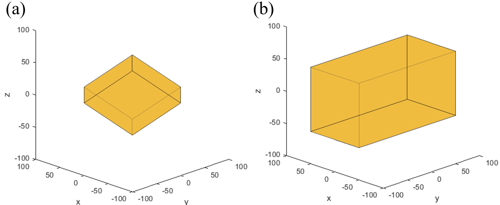
The choice of basis $\bm{V}$ and corresponding parallelepiped is not unique; but, all choices have the same volume, denoted $|\Omega|$ and equal to $|\det(\bm{V})|$. Among all possible $\bm{V}$, we choose the $\bm{V}$ with the smallest condition number, i.e., we choose $\Omega$ closest to a cube to spread the unambiguous velocity coverage in a nearly isotropic manner. However, choices of a parallelepiped with a long and “pointy” shape along a certain direction might be desirable for a specific application. Examples of two possible fundamental parallelepipeds are shown in Fig. 1 for the encoding matrix

$$\bm{A}=2\pi\begin{bmatrix}[r]1&0&0\\ 0&\frac{1}{2}&0\\ 0&0&\frac{1}{3}\end{bmatrix}.$$

(10)

To numerically construct a parallelepiped for the unambiguous range, we set $\widetilde{\bm{\phi}}=\bm{0}$ and search over $\bm{\Lambda}$. The search can be simplified by finding an upper bound on $\Omega$. To handle the case that an element of $\bm{A}$ may be zero, we define $\oslash$ to be the modified element-wise division, and $\overline{\text{lcm}}$ as a generalized least common multiple (lcm) of numbers that can include $0$:

	$\displaystyle\bm{c}$	$\displaystyle=$	$\displaystyle a\oslash\bm{b},\text{where }c_{i}=\begin{cases}\frac{a}{b_{i}},\text{ if }b_{i}\not=0\\ 0,\text{ else}\end{cases}$
	$\displaystyle\overline{\text{lcm}}(\{b_{i}\})$	$\displaystyle=$	$\displaystyle\text{lcm}(\{b_{i}|b_{i}\not=0\}).$		(11)

For convenience, we use $\bm{A}_{:,i}$ and $\bm{A}_{i,:}$ to denote the $i^{th}$ column and row of $\bm{A}$, respectively. Thus, we can observe that if $\bm{A}\bm{v}_{\star}\equiv\bm{0}\mod 2\pi$, then

$\displaystyle\bm{A}\left(\bm{v}_{\star}+\begin{bmatrix}[r]~{}\overline{\text{lcm}}(2\pi\oslash\bm{A}_{:,1})\\ ~{}\overline{\text{lcm}}(2\pi\oslash\bm{A}_{:,2})\\ ~{}\overline{\text{lcm}}(2\pi\oslash\bm{A}_{:,3})\end{bmatrix}\right)\equiv\bm{0}\mod 2\pi.$

(12)

Let $\Delta$ be a hyper-rectangle in $\mathbb{R}^{3}$ with edge along dimension $i$ given by

$\displaystyle\left[-\overline{\text{lcm}}(2\pi\oslash\bm{A}_{:,i}),~{}\overline{\text{lcm}}(2\pi\oslash\bm{A}_{:,i})\right].$

(13)

Observe that basis vectors $\bm{v}_{1},\bm{v}_{2},\bm{v}_{3}\in\Omega\subseteq\Delta$ are solutions to $\bm{A}\bm{v}\equiv\bm{0}\mod 2\pi$. Then we can numerically find solutions of (4) inside $\Delta$ by searching all possible choices of wrapping integers $\bm{k}$ determined by $\left\lfloor\frac{1}{2\pi}\bm{A}\Delta\right\rfloor$, where $\lfloor\cdot\rfloor$ is floor function. Among solutions achieving the minimum volume, we choose one with the smallest condition number, $\kappa(\bm{V})$.

Balanced 4-point encoding uses vertexes of a regular tetrahedron:

$\displaystyle\bm{M}=m\begin{bmatrix}[r]-1&-1&-1\\ +1&+1&-1\\ +1&-1&+1\\ -1&+1&+1\end{bmatrix},\bm{A}=\gamma m\begin{bmatrix}[r]2&2&0\\ 2&0&2\\ 0&2&2\\ 0&-2&2\\ -2&0&2\\ -2&2&0\end{bmatrix}$

(14)

where $m$ is a positive constant. In 1991, Pelc et al. [9] introduced 3-directional flow encoding and pre-processed the phase differences to conveniently yield a decoupled set of three equations in three unknown velocity components. Specifically, the pre-processing is given by $\bm{P}_{91}\in\mathbb{R}^{3\times 6}$:

	$\displaystyle\bm{P}_{91}\bm{A}\bm{v}+\bm{P}_{91}\bm{\epsilon}\equiv\bm{P}_{91}\widetilde{\bm{\phi}}\mod 2\pi$				(15)
	$\displaystyle\bm{P}_{91}=\begin{bmatrix}[r]1&0&0&0&0&-1\\ 1&0&0&0&0&1\\ 0&0&1&1&0&0\end{bmatrix}$				(16)
	$\displaystyle\bm{P}_{91}\bm{A}=\gamma m\begin{bmatrix}[r]4&0&0\\ 0&4&0\\ 0&0&4\end{bmatrix}$	.			(17)

The pre-processing diminishes the information content. Starting from (17), the noise sensitivity is degraded by $3\%$ compared to using all six phase differences, for a signal-to-noise ratio (SNR) of $\sqrt{a_{l}^{2}/\text{var}(n_{l})}=5$. The unambiguous set of velocities is reduced to a cube of edge length $\pi(2\gamma m)^{-1}$.

In 2010, Johnson and Markl [10] proposed a pre-processing that keeps the first three rows of $\bm{A}$, resulting in three coupled equations in three unknowns:

	$\displaystyle\bm{P}_{10}\bm{A}v+\bm{P}_{10}\bm{\epsilon}\equiv\bm{P}_{10}\widetilde{\phi}\mod 2\pi$				(18)
	$\displaystyle\bm{P}_{10}=\begin{bmatrix}[r]1&0&0&0&0&0\\ 0&1&0&0&0&0\\ 0&0&1&0&0&0\end{bmatrix}$				(19)
	$\displaystyle\bm{P}_{10}\bm{A}=\gamma m\begin{bmatrix}[r]2&2&0\\ 2&0&2\\ 0&2&2\end{bmatrix}$	.			(20)

To conveniently eliminate the need for phase unwrapping, the unambiguous set of velocities is defined in [10] such that $-\pi\preccurlyeq\bm{P}_{10}\bm{A}\bm{v}\preccurlyeq\pi$

$$-\pi\preccurlyeq\bm{P}_{10}\bm{A}\bm{v}\preccurlyeq\pi,$$

(21)

where $\preccurlyeq$ is element-wise inequality. Thus, the unambiguous set in [10] is determined by six linear inequalities. The pre-processing slightly worsens noise sensitivity by $6\%$ at SNR of 5,compared to using all six phase differences; interestingly, the pre-processing and restriction in (21) in this case preserve the fundamental parallelepiped for the encoding matrix $\bm{A}$.

In Fig. 2, we illustrate the unambiguous velocity range for 4-point encoding and compare with the pre-processing approaches reviewed above. The pre-processing $\bm{P}_{91}$ leads to a 4 times smaller parallelepiped volume compared to both the fundamental parallelepiped, $\Omega$, and the pre-processing with $\bm{P}_{10}$.

Balanced 5-point encoding [10] augments the balanced 4-point encoding with an additional point at the origin:

$\displaystyle\bm{M}=m\begin{bmatrix}[r]0&0&0\\ -1&-1&-1\\ +1&+1&-1\\ +1&-1&+1\\ -1&+1&+1\end{bmatrix},\bm{A}=\gamma m\small\begin{bmatrix}[r]-1&-1&-1\\ 1&1&-1\\ 1&-1&1\\ -1&1&1\\ 2&2&0\\ 2&0&2\\ 0&2&2\\ 0&-2&2\\ -2&0&2\\ -2&2&0\end{bmatrix}.$

(22)

The pre-processing proposed in [10] for 5-point encoding utilizes the first four equations of $\bm{A}$ to determine the unambiguous velocity range.

	$\displaystyle\bm{P}_{5}\bm{A}v+\bm{P}_{5}\bm{\epsilon}\equiv\bm{P}_{5}\widetilde{\bm{\phi}}\mod 2\pi$		(23)
	$\displaystyle\bm{P}_{5}=\begin{bmatrix}[r]\bm{I}_{4\times 4}&\bm{0}_{4\times 6}\end{bmatrix}$		(24)
	$\displaystyle\bm{P}_{5}\bm{A}=\gamma m\begin{bmatrix}[r]-1&-1&-1\\ 1&1&-1\\ 1&-1&1\\ -1&1&1\end{bmatrix}$		(25)

The four equations in three unknowns are solved least-squares, again with the restriction

$$-\pi\preccurlyeq\gamma\bm{P}_{5}\bm{A}\bm{v}\preccurlyeq\pi.$$

(26)

In Fig. 3, we illustrate the unambiguous velocity range for the $\bm{P}_{5}$ pre-processing with restriction in (26). Using all phase differences leads to $1.5$ times larger volume and $10\%$ better noise sensitivity, compared to the $\bm{P}_{5}$ pre-processing.

We have shown that in phase-contrast-based flow imaging, all phase differences can be processed jointly to maintain the noise sensitivity and full unambiguous range intrinsic to the encoding matrix, $\bm{A}$. In this subsection, we illustrate the potential of utilizing simple lattice concept in Section 2.4 to enable encoding design resulting in an increased unambiguous velocity range, $\Omega$.

For 4-point encoding, we replace the first row of $\bm{M}$ with $\left[-1,\,-0.5,\,-1\right]$ to obtain $\bm{M}^{\prime}$. Then after processing all phase differences, the unambiguous range $\Omega$ for $\bm{M}^{\prime}$ is $4$ times larger than for $\bm{M}$, as illustrated in Fig. 4.

For 5-point encoding, we replace the first row of $\bm{M}$ with $\left[0,\,0,\,0.4\right]$ to obtain $\bm{M}^{\prime}$. Then after processing all phase differences, the unambiguous range $\Omega$ for $\bm{M}^{\prime}$ is $2$ times larger, as illustrated in Fig. 5.

These two examples are suggestive of possible improvements; optimized acquisition would combine unambiguous range given by the parallelepiped $\Omega$, noise sensitivity in (6), and probability of wrapping errors [4]. The optimized design is beyond the scope of this short conference manuscript. In conclusion, we have demonstrated that compared to the existing practice of employing a pre-processing step, jointly processing all phase differences leads to a larger unambiguous velocity range and higher VNR.

References

- [1] Norbert J Pelc, Robert J Herfkens, Ann Shimakawa, Dieter R Enzmann, et al., “Phase contrast cine magnetic resonance imaging,” Magn. Reson. Q., vol. 7, no. 4, pp. 229–254, 1991.
- [2] Michael Markl, Alex Frydrychowicz, Sebastian Kozerke, Mike Hope, and Oliver Wieben, “4D flow MRI,” J. Magn. Reson. Imaging, vol. 36, no. 5, pp. 1015–1036, 2012.
- [3] Adam Rich, Lee C Potter, Ning Jin, Joshua Ash, Orlando P Simonetti, and Rizwan Ahmad, “A Bayesian model for highly accelerated phase-contrast MRI,” Magn. Reson. Med., vol. 76, no. 2, pp. 689–701, 2016.
- [4] Shen Zhao, Rizwan Ahmad, and Lee C Potter, “Venc design and velocity estimation for phase contrast MRI,” arXiv preprint arXiv:2109.12481, 2021.
- [5] Carl Friedrich Gauss, Disquisitiones arithmeticae, Translated into English by Arthur A. Clarke, S. J. Yale University Press, New Haven, Conn., 1966.
- [6] Thomas M. Cover and Joy A. Thomas, Elements of Information Theory, pp. 34–35, Wiley-Interscience, USA, 2006.
- [7] Alexander Barvinok, “Math 669: Combinatorics, Geometry, and Complexity of Integer Points,” www.math.lsa.umich.edu/~barvinok/c20.html, Accessed: 2021-10-11.
- [8] Oliver Knill, “A multivariable Chinese remainder theorem,” arXiv preprint arXiv:1206.5114, 2012.
- [9] Norbert J Pelc, Matt A Bernstein, Ann Shimakawa, and Gary H Glover, “Encoding strategies for three-direction phase-contrast MR imaging of flow,” J. Magn. Reson. Imaging, vol. 1, no. 4, pp. 405–413, 1991.
- [10] Kevin M Johnson and Michael Markl, “Improved SNR in phase contrast velocimetry with five-point balanced flow encoding,” Magn. Reson. Med., vol. 63, no. 2, pp. 349–355, 2010.