^a^ainstitutetext: Theory Center, Institute of Particle and Nuclear Studies, KEK
Tsukuba, Ibaraki, 305-0801, Japan^b^binstitutetext: National Institute of Technology, Kurume College,
Kurume, Fukuoka, 830-8555, Japan

Matter from multiply enhanced singularities in F-theory

Shun’ya Mizoguchi b and Taro Tani [email protected] [email protected]

(July 20, 2024)

Abstract

We investigate the geometrical structure of multiply enhanced codimension-two singularities in the $SU(5)$ model of six-dimensional F-theory, where the rank of the singularity increases by two or more. We perform blow-up processes for the enhancement $SU(5)\rightarrow G^{\prime}$ , where $G^{\prime}=E_{6}$ , $E_{7}$ or $E_{8}$ , to examine whether a sufficient set of exceptional curves emerge that can explain the charged matter generation predicted from anomaly cancelation. We first apply one of the six Esole-Yau small resolutions to the multiply enhanced singularities, but it turns out that the proper transform of the threefold equation does not reflect changes in the singularity or how the generic codimension-two singularities gather there. We then use a(n) (apparently) different way of small resolutions than Esole-Yau to find that, except for the cases of $G^{\prime}=E_{6}$ and special cases of $E_{7}$ , either (1) the resolution only yields exceptional curves that are insufficient to cancel the anomaly, or (2) there arises a type of singularity that is neither a conifold nor a generalized conifold singularity. Finally, we revisit the Esole-Yau small resolution and show that the change of the way of small resolutions amounts to simply exchanging the proper transform and the constraint condition, and under this exchange the two ways of small resolutions are completely equivalent.

^†^†preprint: KEK-TH-2637

1 Introduction

There is no doubt that singularities play an essential role in F-theory. It is basically formulated on an elliptically fibered complex manifold on some base, where the elliptic fiber modulus represents the value of the complex scalar field $\tau$ of type IIB string theory Vafa . Depending on its complex structure, a singularity may arise somewhere on the fiber. From the perspective of type IIB theory compactified on the base, this is where a 7-brane exists. More precisely, a 7-brane resides at a locus on the base over which the fiber develops a singularity. As branes overlap or intersect each other to achieve gauge symmetry or matter in string theory MV1 ; MV2 ; BIKMSV , the structure of the singularities in F-theory determines how they are geometrically realized.

On an elliptic surface, the types of singularities are classified by Kodaira Kodaira . Precisely speaking, it classifies the types of the set of exceptional fibers that arise through the process of resolving a singularity. As is well known, Kodaira’s fiber type is specified by, except for a few exceptional cases, an extended Dynkin diagram of some simple Lie algebra representing how $\hbox{\mybb P}^{1}$ ’s arising as exceptional sets intersect each other. So each fiber type is naturally associated with some simple Lie algebra $G$ ; its fiber type is often specified by this Lie algebra $G$ or its corresponding Dynkin diagram, just like the du Val-Kleinian $ADE$ singularities, rather than by the original name of Kodaira’s fiber type. We will also use this terminology to refer to these singularities in this paper. In the literature, such a singularity is often called a codimension-one singularity¹¹1 We should note that the usage of this term is somewhat misleading; what is actually codimension-one is the locus on the base of the elliptic fibration, but the actual singularity lies on the fiber over such a locus. Therefore, while this terminology is appropriate for the type IIB (or F-GUT DonagiWijnholt ; BHV1 ; BHV2 ; DonagiWijnholt2 ) perspective, from the F-theory perspective it would be more reasonable to say that this singularity is codimension-two, counting the codimensions in the total elliptic space. However, in this paper, following EsoleYau , we will (somewhat misleadingly) refer to this as a codimension-one singularity, which is the same terminology as in much of the literature on F-GUT. .

If one fibers such elliptic surfaces over some base manifold $\cal B$ , one can obtain a higher-dimensional elliptic manifold whose base is a $\hbox{\mybb P}^{1}$ fibration over ${\cal B}$ , on which one can consider F-theory. In six-dimensional F-theory, the base of the elliptic fibration is complex two-dimensional, so codimension-one discriminant loci intersect each other generically at isolated points. As is well known, matter emerges from these codimension-two singularities²²2Again, what is codimension-two is the locus on the base, and the singularity itself on the elliptic manifold is codimension three. Still, we call it codimension-two similarly. KatzVafa ; BIKMSV , and on the fiber over such loci, the $G$ singularity over the generic codimension-one loci changes into a different $G^{\prime}$ singularity of higher rank. The change in the rank from $G$ to $G^{\prime}$ is one generically.

In this paper, we consider codimension-two singularities in six-dimensional F-theory, where the rank of the singularity $G^{\prime}$ is two or more higher than that of the generic co-dimension-one singularity $G$ around it. We will call such a change in the rank of the Lie algebras of the singularities “multiple enhancement”. In six dimensions, these multiply enhanced codimension-two singularities do not generically occur, but appear only when the complex structure moduli are specifically tuned so that several generic codimension-two singularities happen to overlap. In the intersecting 7-brane picture, this corresponds to the case where two branes no longer intersect transversally.

In a generic rank-one enhancement from $G$ to $G^{\prime}$ in six dimensions, massless matter arising there can be understood as coming from light M2-branes KatzVafa wrapped around extra two-cycles that newly emerge over the enhanced point. An understanding of matter generation in terms of string junction was discussed in Tani . In typical cases, these massless states correspond to one of the roots of $G^{\prime}$ . In particular, if there is no monodromy among these two-cycles (the “split” case), the massless matter arising there is given by $G^{\prime}/(G\times U(1))$ , which forms a homogeneous Kähler manifold. As was investigated in detail in BIKMSV , if the base space of the elliptic fibration is taken to be a Hirzebruch surface MV1 ; MV2 , the set of matter multiplets given by this rule coincides exactly with those of $E_{8}\times E_{8}$ heterotic string on a K3 surface, in particular all anomalies cancel. On the other hand, as mentioned above, a singularity that enhances the rank by two or more occurs when several ordinary rank-one enhanced singularities come together and overlap. This means that, at such special points on the moduli space, the massless matter hypermultiplets arising from some of the ordinary rank-one enhanced singularities that existed disappear, and a new set of massless matter hypermultiplets is created at the multiply enhanced singularity.

In six dimensions, however, the constraints for anomaly cancelation are very strict so that the changes in the spectrum of massless matter are severely restricted. Indeed, anomaly cancellation requires that there should be no net change in the number of hypermultiplets in such transitions MTanomaly . This is simply because the Green-Schwarz mechanism in six dimensions GSW ; Sadov requires that the numbers of vector, tensor and hypermultiplets $n_{V}$ , $n_{T}$ and $n_{H}$ satisfy

\displaystyle n_{H}-n_{V}

\displaystyle=

\displaystyle 273-29n_{T}.

(1)

Therefore, the number of hypermultiplets cannot change unless the number of multiplets in vectors and tensors does not change (which is assumed here)³³3In general, a different representation contributes differently to the anomalies, so the number of hypermultiplets in each representation must be the same before and after the transition.. This prohibition on the change in the number of hypermultiplets in turn predicts what charged hypermultiplets occur from such a singularity with a multiple enhancement. The purpose of this paper is to examine whether the massless matter predicted in this way can be understood from the geometric structure of the singularity with a multiple enhancement.

In this paper we revisit the well-studied compactification of six-dimensional F-theory on Hilzebruch surfaces $\hbox{\mybb F}_{n}$ MV1 ; MV2 ; BIKMSV with unbroken $SU(5)$ gauge symmetry. We will explicitly carry out the resolution process in the cases of multiple enhancements $SU(5)\rightarrow E_{6}$ , $E_{7}$ and $E_{8}$ to see whether the expected matter spectrum can be explained in terms of exceptional curves arising from the resolutions. We are interested in the local structure of the singularity, so although we work in this particular global set-up, the result will apply to any six-dimensional F-theory compactification.

The singularity structure of the four-dimensional F-theory $SU(5)$ model compactified on a Calabi-Yau fourfold was analyzed in EsoleYau , and very impressive results were revealed. (See also relatedanalysis1 ; relatedanalysis2 ; relatedanalysis3 ; relatedanalysis4 ; relatedanalysis5 .) starting with the $SU(5)$ equation in Tate’s form, two-time codimension-one blow-ups yield an equation in the “binomial” form, that is, the equation for the threefold after the two blow-ups takes the form

\displaystyle u_{1}u_{2}u_{3}-v_{1}v_{2}

\displaystyle=

\displaystyle 0,

(2)

where $u_{1},\ldots,v_{2}$ are sections of some relevant line bundles (see later sections for details). The equation (2) indicates that, if $v_{1}$ , $v_{2}=0$ and two (and only two) of the three sections $u_{1}$ , $u_{2}$ and $u_{3}$ simultaneously vanish, there is a conifold singularity. This is the place where a codimension-two singularity resides; after the codimension-one blow-ups, conifold singularities remain at the codimension-two loci (in the sense of the base as we remarked). Note that, in four-dimensional F-theory considered in EsoleYau , these conifold singularities form complex curves such as discussed in ConifoldTransitionsinMtheory .

It was found in EsoleYau that, generically, these conifold singularities are all disingularized by successive two small resolutions inserting two curves of $\hbox{\mybb P}^{1}$ ’s replacing the curves of singularities. There are six ways to do this, depending on which of $u_{i}$ ’s is paired with $v_{1}$ or $v_{2}$ . For instance, this is done by replacing, say, $(v_{1},u_{1})$ and $(v_{2},u_{2})$ with

	$\displaystyle v_{1}=\xi V_{1},~{}~{}~{}u_{1}=\xi U_{1},$		(3)
	$\displaystyle v_{2}=\zeta V_{2},~{}~{}~{}u_{2}=\zeta U_{2},$		(4)

where $(V_{1}:U_{1})$ and $(V_{2}:U_{2})$ are the homogeneous coordinates of $\hbox{\mybb P}^{1}$ ’s mentioned above, and $\xi$ and $\zeta$ are sections of appropriate line bundles served for projectivization⁴⁴4 $\xi$ , $\zeta$ here were denoted as $\delta_{3}$ , $\delta_{4}$ in Yukawas , respectively..

This also applies to the present six-dimensional case. Again, in the generic case where there is no multiple enhancement, all the codimension-two conifold singularities are resolved in this way. However, in the case of multiple enhancement, a different type of singularity appears than a conifold singularity, at which all three $u_{i}$ ’s vanish simultaneously. In fact, such singularities are also known to appear in generic four-dimensional models: The codimension-three $E_{6}$ singularity. In this four-dimensional case, even such non-conifold singularities are readily resolved by the above two small resolutions EsoleYau ; Yukawas . In six dimensions, on the other hand, there is no such thing as “codimension-three” singularity (since the base is two-dimensional) but such singularities appear only when the complex structure is properly tuned.

We will perform the resolution of this kind of singularity in two different ways. A difference occurs after the two codimension-one blow-ups⁵⁵5 In fact, the first small resolutions ((3) and (5)) performed after the codimension-one blow-ups are the same, so the difference arises in the second small resolutions.. One way is through two small resolutions (3)(4) done in EsoleYau as described above. As we will see, it turns out that if we do this, we run into something strange: Even in the case of multiple enhancements, it ends up looking like nothing special is happening. So we consider an alternative way of small resolutions: We perform the same first small resolution (3) as above, but for the second small resolution we insert $\hbox{\mybb P}^{1}$ at $V_{1}=u_{3}=0$ :

	$\displaystyle v_{1}=\xi V_{1},~{}~{}~{}u_{1}=\xi U_{1},$		(5)
	$\displaystyle V_{1}=\eta V^{\prime}_{1},~{}~{}~{}u_{3}=\eta U_{3}.$		(6)

This change of the center of the blow up leads to an equivalent small resolution for ordinary conifold singularities. However, we will see that there is indeed a difference between (4) and (6) when we actually apply the resolution procedure to a multiply enhanced singularity.

We will then revisit the first way of small resolutions (4). We will show what was overlooked and why it looked like “nothing happened” then. In fact, if we properly consider what we missed, we will see that the two ways of small resolutions are again equivalent for multiply enhanced singularities as well, and exactly the same conclusions can be drawn from both. This equivalence is realized in a rather interesting way as a certain “duality”, in which the proper transform of the threefold equation in one way of small resolutions corresponds to the constraint equation in the other.

The organization of this paper is as follows. In section 2, we list possible realizations of singularities to achieve each multiple enhancement. We also examine how many hypermultiplets are expected to arise there to cancel the anomalies. In section 3, we apply the Esole-Yau small resolution (3)(4) to those singularities and find that, in all cases, the proper transform after the two-time codimension-one blow-ups is regular. In section 4, we use the alternative small resolution (5)(6) and show that, in this procedure, the proper transforms reflect changes in the singularity. We find that, except for the case of $G^{\prime}=E_{6}$ and special cases of $G^{\prime}=E_{7}$ , either (1) the resolution only yields exceptional curves that are insufficient to cancel the anomaly, or (2) there arises a type of singularity that is neither a conifold nor a generalized conifold singularity⁶⁶6One can show that these phenomena are not specific to $SU(5)\rightarrow E_{n}$ , but common to multiple enhancements. In particular, a simple example of (1) is $SU(2)\rightarrow SO(8)$ .. In section 5, we revisit the Esole-Yau small resolution and find that there is a “duality” between the two ways of small resolution, showing that they are equivalent.

2 Multiply enhanced singularities in 6D F-theory

2.1 Tate’s form and multiply enhanced singularities

We consider six-dimensional compactifications of F-theory on Calabi-Yau threefolds (CY₃), which are elliptically fibered over a Hirzebruch surface $\hbox{\mybb F}_{n}$ . Let $z$ and $w$ are affine coordinates of the fiber $\hbox{\mybb P}^{1}$ and the base $\hbox{\mybb P}^{1}$ in the relevant coordinate patch of $\hbox{\mybb F}_{n}$ , respectively. We describe such a CY₃ in Tate’s form

y^{2}+a_{1}xy+a_{3}y=x^{3}+a_{2}x^{2}+a_{4}x+a_{6}.

(7)

$a_{i}$ ’s are polynomials of the coordinates $(z,w)$ of $\hbox{\mybb F}_{n}$ of particular degrees, representing the sections of appropriate line bundles that satisfy the Calabi-Yau condition. Such a CY₃ can also be seen as a K3 fibered geometry over the base $\hbox{\mybb P}^{1}$ of $\hbox{\mybb F}_{n}$ .

To achieve a split $SU(5)$ model BIKMSV , we assume the orders of the sections in $z$ as

{\rm o}(a_{1}\,,a_{2},\,a_{3},\,a_{4},\,a_{6})=(0,1,2,3,5),

(8)

where we write the order of the polynomial $a_{i}(z)$ in $z$ as ${\rm o}(a_{i})$ . They are realized by assuming

\begin{split}a_{1}&=a_{1,0}+a_{1,1}z+\cdots,\\ a_{2}&=a_{2,1}z+a_{2,2}z^{2}+\cdots,\\ a_{3}&=a_{3,2}z^{2}+a_{3,3}z^{3}+\cdots,\\ a_{4}&=a_{4,3}z^{3}+a_{4,4}z^{4}+\cdots,\\ a_{6}&=a_{6,5}z^{5}+a_{6,6}z^{6}+\cdots,\end{split}

(9)

where $a_{i,j}$ are polynomials of $w$ . The leading terms are sufficient to describe the relevant structure of the singularity. The independent polynomials defining the $SU(5)$ singularity are

\displaystyle a_{1,0},\,a_{2,1},\,a_{3,2},\,a_{4,3},\,a_{6,5},

(10)

and (7) reads (to leading order in $z$ for each $a_{i}$ )

\displaystyle y^{2}+a_{1,0}xy+a_{3,2}z^{2}y=x^{3}+a_{2,1}zx^{2}+a_{4,3}z^{3}x+a_{6,5}z^{5}.

(11)

The corresponding Weierstrass equation is given by

\displaystyle y^{2}=x^{3}+fx+g

(12)

with

\begin{split}f&=-\frac{1}{48}a_{1,0}^{4}+\left(-\frac{1}{6}a_{1,0}^{2}a_{2,1}+\cdots\right)z+\left(-\frac{1}{6}(2a_{2,1}^{2}-3a_{1,0}a_{3,2})+\cdots\right)z^{2}\\ &+(a_{4,3}+\cdots)z^{3}+\cdots,\\ g&=\frac{1}{864}a_{1,0}^{6}+\left(\frac{1}{72}a_{1,0}^{4}a_{2,1}+\cdots\right)z+\left(\frac{1}{72}a_{1,0}^{2}(4a_{2,1}^{2}-3a_{1,0}a_{3,2})+\cdots\right)z^{2}\\ &+\left(\frac{1}{108}(8a_{2,1}^{3}-18a_{1,0}a_{2,1}a_{3,2}-9a_{1,0}^{2}a_{4,3})+\cdots\right)z^{3}\\ &+\left(\frac{1}{12}(3a_{3,2}^{2}-4a_{2,1}a_{4,3})+\cdots\right)z^{4}+(a_{6,5}+\cdots)z^{5}+\cdots.\end{split}

(13)

The discriminant is given by

\begin{split}\Delta&=4f^{3}+27g^{2}\\ &=\frac{1}{16}\big{(}a_{1,0}^{4}\,P_{8,5}\,z^{5}+a_{1,0}^{2}\,Q_{10,6}\,z^{6}+R_{12,7}z^{7}+\cdots\big{)},\end{split}

(14)

where

\begin{split}P_{8,5}&=a_{2,1}a_{3,2}^{2}-a_{1,0}a_{3,2}a_{4,3}+a_{1,0}^{2}a_{6,5},\\ Q_{10,6}&=8a_{2,1}^{2}a_{3,2}^{2}+(\mbox{terms divisible by}\,\,a_{1,0}),\\ R_{12,7}&=16a_{2,1}^{3}a_{3,2}^{2}+(\mbox{terms divisible by}\,\,a_{1,0}).\end{split}

(15)

The orders of $f,g$ and $\Delta$ are generically given by $\mbox{o}(f,g,\Delta)=(0,0,5)$ and the $SU(5)$ singularity is realized at the codimansion-one locus $z=0$ .

The degrees in $w$ of the independent polynomials (10) depend on $n$ of $\hbox{\mybb F}_{n}$ and are given by

\mbox{deg}(a_{i,j})=n\,(i-j)+2i.

(16)

Writing explicitly:

\mbox{deg}(a_{1,0},\,a_{2,1},\,a_{3,2},\,a_{4,3},\,a_{6,5})=(n+2,\,n+4,\,n+6,\,n+8,\,n+12).

(17)

The number of neutral hypermultiplets is thus

n_{H0}=(n+3)+(n+5)+(n+7)+(n+9)+(n+13)-1=5n+36.

(18)

Charged hypermultiplets are localized at codimension-two discriminant loci, where the singularity gets enhanced. At $a_{1,0}=0$ , one can see from (13) and (14) that $\mbox{o}(f,g,\Delta)=(2,3,7)$ , thus the enhancement $SU(5)\rightarrow SO(10)$ occurs (see Table 1 for the Weierstrass orders in the Kodaira classification). Correspondingly, a chiral matter in $\mathbb{10}$ is localized at each point of $a_{1,0}=0$ . Also, at $P_{8,5}=0$ , $\mbox{o}(f,g,\Delta)=(0,0,6)$ and the enhancement $SU(5)\rightarrow SU(6)$ occurs. It gives a chiral matter in $\mathbb{5}$ localized at $P_{8,5}=0$ . Note that both of them are rank-one enhancements. Since $a_{1,0}$ and $P_{8,5}$ have degrees $n+2$ and $3n+16$ , respectively, we obtain the charged matter spectrum

(n+2)\mathbb{10}\oplus(3n+16)\mathbb{5}.

(19)

The number of the charged hypermultiplets is thus

n_{Hc}=(n+2)\times 10+(3n+16)\times 5=25n+100,

(20)

which gives the number of hypermultiplets as

n_{H}=n_{H0}+n_{Hc}=30n+136,

(21)

satisfying the anomaly-free condition MV1

n_{H}-n_{V}=30n+112

(22)

with the number of vector multiplets $n_{V}=24$ for $SU(5)$ .

Additional conditons on $a_{ij}$ ’s yield multiple enhancements (rank $\geq$ 2 enhancements). The conditions for realizing the enhancements to $SO(12)$ and $E_{n}$ ( $n=6,7,8$ ) can be read from (13), (14) and (15) and are summarized in Table 1.

Singularity	$\mbox{o}(f)$	o(g)	$\mbox{o}(\Delta)$	Conditions for $a_{i,j}$ (Tate’s orders)
$SU(5)$	0	0	5
$SU(6)$	0	0	6	$P_{8,5}=0$
$SO(10)$	2	3	7	$a_{1,0}=0$
$SO(12)$	2	3	8	$a_{1,0}=a_{3,2}=0$
$E_{6}$	$\geq$ 3	4	8	$a_{1,0}=a_{2,1}=0$
$E_{7}$	3	$\geq$ 5	9	$a_{1,0}=a_{2,1}=a_{3,2}=0$
$E_{8}$	$\geq$ 4	5	10	$a_{1,0}=a_{2,1}=a_{3,2}=a_{4,3}=0$

Table 1: rank-one and rank

\geq 2

enhancements of

SU(5)

2.2 Incomplete/Complete multiply enhanced singularities

Even if the Lie algebra to which the singularity is enhanced is specified, there are variety of possibilities in achieving the enhancement in general. For example, let us consider the rank-two enhancement $SU(5)\rightarrow E_{6}$ . This enhancement is a generic one in four dimensions, but in six dimensions it only occurs if the complex structure is so tuned, as we mentioned. The condition for this enhancement is

\displaystyle a_{1,0}=a_{2,1}=0.

(23)

Since $a_{1,0}=0$ is the condition for the enhancement to $SO(10)$ , this is where a 10 hypermultiplet arises. If $a_{2,1}=0$ is further satisfied, $P_{8,5}$ will also become $0$ , so this is also the place where a 5 appears as localized matter. Thus we see that an $E_{6}$ point⁷⁷7We say that a point on the two-dimensional base ( $=\hbox{\mybbsub F}_{n}$ in the present case) of the elliptic fibration is a $G$ point if the elliptic fiber over that point develops a $G$ singularity in the sense of Kodaira as a singularity of a surface (in the present case the fiber K3 surface of the K3 fibration over the base $\hbox{\mybbsub P}^{1}$ of $\hbox{\mybbsub F}_{n}$ ). can be made up of an $SO(10)$ point and an $SU(6)$ point overlapping each other. Since the condition only requires that $a_{1,0}$ or $a_{2,1}$ be zero there, their orders in $w$ are arbitrary. Therefore, we may alternatively assume that $a_{1,0}$ has a double root ${\rm o}_{w}(a_{1,0})=2$ there, where we denote the order of the polynomial $a_{i,j}(w)$ by ${\rm o}_{w}(a_{i,j})$ . Then, a slight deformation of the complex structure will result in two single roots of $a_{1,0}=0$ that are close to each other, at each of which a hypermultiplet 10 occurs. Put in the reverse direction, such a multiply enhanced point arises from two $SO(10)$ points and one $SU(6)$ point. Therefore, two 10 and one 5 must be generated there to remain free of anomalies.

This is reminiscent of the case of the ordinary rank-one enhancement from $SU(6)$ to $E_{6}$ , where a generic codimension-two singularity generates half-hypermultiplets MT . In that case, let $t_{r}$ be the relevant section (in the notation of halfhyper ), then if ${\rm o}_{w}(a_{1,0})=1$ , a single half-hypermultiplet 20 of $SU(6)$ appears, while if ${\rm o}_{w}(a_{1,0})=2$ , there arise two half-hypermultiplets to form a full hypermultiplet. It was found MT that, in the latter case, there appears an additional conifold singularity, and an extra exceptional curve arising through the resolution “completes” the full $E_{6}$ Dynkin diagram. A related analysis was done in Yukawas , and other cases where massless half-hypermultiplets are generated were investigated in halfhyper .

In the present $SU(5)$ models, if the enough number of exceptional curves arise to form the full $E_{6}$ Dynkin diagram, then one might similarly expect that

\displaystyle E_{6}/(SU(5)\times U(1)^{2})

\displaystyle=

\displaystyle{\bf 10}\oplus{\bf 10}\oplus{\bf 5}\oplus{\bf 1}

(24)

arise as localized matter there. On the right side here and below, the 5 and the ${\bf\bar{5}}$ are denoted interchangeably as a hypermultiplet. We call such a codimension-two $E_{6}$ singularity (enhanced from $SU(5)$ ) made of two 10’s and one 5 a complete singularity, whereas one made of a single 10 and a single 5 an incomplete singularity⁸⁸8In MT , the terms complete/incomplete resolutions were used; we will slightly change the nomenclature because what is incomplete is not the process of resolution and so it is somewhat misleading.. (In this paper, we ignore the match of the number of singlets, focusing only the change of the numbers of charged hypermultiplets.)

In the cases where half-hypermultiplets are involved, the change in the structure of the singularity successfully explains the matter generation expected to occur there MT ; halfhyper . So, then, in the case of multiple enhancement where ordinary hypermultiplets (that is, full hypermultiplets that are not half ones) gather, is there also a singularity structure that can account for the matter generation of that much? This is the question that we would like to address in this paper.

2.3 Incomplete singularities in $SU(5)\rightarrow E_{6}$ , $E_{7}$ and $E_{8}$

Similarly, we define a complete singularity in the enhancement to $G^{\prime}=E_{7}$ and $E_{8}$ as one made up of generic codimension-two singularities that generate the same set of charged hypermultiplets as $G^{\prime}/(SU(5)\times U(1)^{{\rm rank}G^{\prime}-4})$ . If, on the other hand, an $G^{\prime}=E_{7}$ or $E_{8}$ singularity made of a coalescence of generic singularities that support smaller number of hypermultiplets will be called an incomplete singularity.

As we saw in the previous subsection, how many hypermultiplets (or rather, how many generic codimension-two singularities that generate them) gather is determined by the order in $w$ of relevant sections that vanish there. In the following, we will examine each case of $G^{\prime}=E_{6},E_{7}$ , and $E_{8}$ in turn to see what they are in detail.

$SU(5)\rightarrow E_{6}$

As we have already seen in the previous subsection, we can distinguish two cases:

$\mbox{o}_{w}(a_{1,0})$	$\mbox{o}_{w}(a_{2,1})$	$\mbox{o}_{w}(a_{3,2})$	$\mbox{o}_{w}(a_{4,3})$	$\mbox{o}_{w}(a_{6,5})$	$\mbox{o}_{w}(P_{8,5})$	name
$1$	$1$	$0$	$0$	$0$	$1$	incomplete
$2$	$1$	$0$	$0$	$0$	$1$	complete

Table 2:

E_{6}

patterns.

Of course, we could consider further patterns in which more general codimension-two singularities overlap than in the complete case, but we limit ourselves to these cases in this paper. Also, we note that the orders of $P_{8,5}$ are calculated for generic sections $a_{1,0},\ldots,a_{6,5}$ with the specified orders; they can be accidentally larger than them if $a_{1,0},\ldots,a_{6,5}$ satisfy some relation.

$SU(5)\rightarrow E_{7}$

If a set of exceptional curves occurs such that the intersection diagram coincides with the complete $E_{7}$ Dinkin diagram, then the resulting hypermultiplets will be

\displaystyle E_{7}/(SU(5)\times U(1)^{3})

\displaystyle=

\displaystyle 3\cdot{\bf 10}\oplus 4\cdot{\bf 5}\oplus 3\cdot{\bf 1},

(25)

where, again, ${\bf 5}$ and ${\bf\bar{5}}$ are identified as the same hypermultiplet. Thus we define a complete $E_{7}$ singularity as an $E_{7}$ singularity where $\mbox{o}_{w}(a_{1,0})=3$ , $\mbox{o}_{w}(P_{8,5})=4$ , and $\mbox{o}_{w}(a_{2,1})$ , $\mbox{o}_{w}(a_{3,2})$ , $\mbox{o}_{w}(a_{4,3})$ and $\mbox{o}_{w}(a_{6,5})$ take minimum values. We also define various incomplete $E_{7}$ singularities as ones with $1\leq\mbox{o}_{w}(a_{1,0})\leq 3$ and $2\leq\mbox{o}_{w}(P_{8,5})\leq 4$ such that $\mbox{o}_{w}(a_{2,1})$ , $\mbox{o}_{w}(a_{3,2})$ , $\mbox{o}_{w}(a_{4,3})$ and $\mbox{o}_{w}(a_{6,5})$ have minimum values for each fixed pair of $\mbox{o}_{w}(a_{1,0})$ and $\mbox{o}_{w}(P_{8,5})$ . Four such incomplete singularities can be found, and they are listed in Table 3 together with the complete singularity.

$\mbox{o}_{w}(a_{1,0})$	$\mbox{o}_{w}(a_{2,1})$	$\mbox{o}_{w}(a_{3,2})$	$\mbox{o}_{w}(a_{4,3})$	$\mbox{o}_{w}(a_{6,5})$	$\mbox{o}_{w}(P_{8,5})$	name
$1$	$1$	$1$	$0$	$0$	$2$	incomplete 1
$2$	$1$	$1$	$0$	$0$	$3$	incomplete 2
$2$	$1$	$2$	$0$	$0$	$4$	incomplete 3
$3$	$1$	$1$	$0$	$0$	$3$	incomplete 4
$3$	$2$	$1$	$0$	$0$	$4$	complete

Table 3:

E_{7}

patterns.

$SU(5)\rightarrow E_{8}$

We can similarly list 45 patterns of complete and incomplete singularities. In fact, we will see later that the details of Tate’s orders for each pattern are not very relevant to the analysis of the resolution. Since it is not very informative, we leave the results to Appendix A.

In the $E_{8}$ case

\displaystyle E_{8}/(SU(5)\times U(1)^{4})

\displaystyle=

\displaystyle 5\cdot{\bf 10}\oplus 10\cdot{\bf 5}\oplus 10\cdot{\bf 1},

(26)

so a complete $E_{8}$ singularity should have $\mbox{o}_{w}(a_{1,0})=5$ and $\mbox{o}_{w}(P_{8,5})=10$ . There are five such patterns, all named complete singularities in Table 4 in Appendix A.

3 Resolution of multiply enhanced singularities in 6D F-theory I : Esole-Yau resolution

3.1 Generalities of the resolution of 6D $SU(5)$ models

In this section, we summarize the general aspects of singularity resolution in 6D $SU(5)$ F-theory models. This also enables us to state the results of EsoleYau on the structure of the $SU(5)$ models in our notation, with some appropriate modifications to six dimensions.

As we said, we work on an elliptic CY threefold over a Hirzebruch surface (11). By moving the terms on the left-hand side, let us write the equation as

\displaystyle\Phi(x,y,z,w)

\displaystyle\equiv

\displaystyle-(y^{2}+a_{1,0}xy+a_{3,2}z^{2}y)+x^{3}+a_{2,1}zx^{2}+a_{4,3}z^{3}x+a_{6,5}z^{5}~{}=~{}0.

(27)

$(x,y,z,w)=(0,0,0,\mbox{any})$ is the codimension-one $SU(5)$ singularity at generic $w$ . As is well known, it is desingularized by two-time insertions of lines of $\hbox{\mybb P}^{2}$ ’s along $(x,y,z)=(0,0,0)$ with arbitrary $w$ . This is done by setting

\displaystyle(x,y,z)

\displaystyle=

\displaystyle(x_{1}z,y_{1}z,z)

(28)

the first time, and

\displaystyle(x_{1},y_{1},z)

\displaystyle=

\displaystyle(x_{1},x_{1}y_{2},x_{1}z_{2})

(29)

the second time⁹⁹9To be completely precise, (28) is a particular expression of the $\hbox{\mybbsub P}^{2}$ blow-up $(x,y,z)=(\delta_{1}X_{1},\delta_{1}Y_{1},\delta_{1}Z_{1})$ , $(X_{1}:Y_{1}:Z_{1})\in\hbox{\mybbsub P}^{2}$ in the patch $Z_{1}\neq 0$ , where $(x_{1}:y_{1}:1)=(X_{1}:Y_{1}:Z_{1})$ are (the former) the affine coordinates in this patch, and $z$ itself becomes the variable for projectivization $\delta_{1}$ . Similarly, (29) is the expression of the blow-up $(x_{1},y_{1},z)=(\delta_{2}X_{2},\delta_{2}Y_{2},\delta_{2}Z_{2})$ , $(X_{2}:Y_{2}:Z_{2})\in\hbox{\mybbsub P}^{2}$ in the patch $X_{2}\neq 0$ . . By plugging (28) into (27), we define

	$\displaystyle\Phi_{z}(x_{1},y_{1},z,w)$	$\displaystyle\equiv$	$\displaystyle z^{-2}\Phi(x_{1}z,y_{1}z,z,w)$
		$\displaystyle=$	$\displaystyle-y_{1}(y_{1}+a_{1,0}x_{1}+a_{3,2}z)+z(x_{1}^{3}+a_{2,1}x_{1}^{2}+a_{4,3}zx_{1}+a_{6,5}z^{2})=0,$

which is called the proper transform. Note that by factoring out $z^{2}$ , the canonical class is preserved so that the new threefold $\Phi_{z}(x_{1},y_{1},z,w)=0$ remains a Calabi-Yau. Likewise we use (29) in (LABEL:Phiz) to obtain

	$\displaystyle\Phi_{zx}(x_{1},y_{2},z_{2},w)$	$\displaystyle\equiv$	$\displaystyle x_{1}^{-2}\Phi_{z}(x_{1},x_{1}y_{2},x_{1}z_{2},w)$
		$\displaystyle=$	$\displaystyle-y_{2}(y_{2}+a_{1,0}+a_{3,2}z_{2})+x_{1}z_{2}(x_{1}+a_{2,1}+a_{4,3}z_{2}+a_{6,5}z_{2}^{2})=0.$

Again, factoring out $x_{1}^{2}$ yields a “crepant” resolution, meaning that it does not change the canonical class.

We performed the second blow-up (29) because $\Phi_{z}(x_{1},y_{1},z,w)=0$ is singular at $(x_{1},y_{1},z)=(0,0,0)$ for arbitrary $w$ . Then after the second blow-up, the new threefold defined by the equation $\Phi_{zx}(x_{1},y_{2},z_{2},w)=0$ is regular except for codimension-two discrete loci on the base, on the fibers over which conifold singularities appear EsoleYau ; MT . This can be clearly seen by rewriting (LABEL:Phizx) as

\displaystyle u_{1}u_{2}u_{3}-v_{1}v_{2}

\displaystyle=

\displaystyle 0

(32)

with

$\displaystyle u_{1}$	$\displaystyle=$	$\displaystyle x_{1},$
$\displaystyle u_{2}$	$\displaystyle=$	$\displaystyle z_{2},$
$\displaystyle u_{3}$	$\displaystyle=$	$\displaystyle x_{1}+a_{2,1}+a_{4,3}z_{2}+a_{6,5}z_{2}^{2}.$
$\displaystyle v_{1}$	$\displaystyle=$	$\displaystyle y_{2},$
$\displaystyle v_{2}$	$\displaystyle=$	$\displaystyle y_{2}+a_{1,0}+a_{3,2}z_{2}.$	(33)

We have already shown these equations as (2) in Introduction.

From (32), we can see that there are three types of conifold singularities in a generic six-dimensional $SU(5)$ model:

•

$v_{1}=v_{2}=0$ and $u_{1}=u_{2}=0$
This occurs if $a_{1,0}=0$ . In this case $y_{2}=x_{1}=z_{2}=0$ . In generic cases where $a_{2,1}\neq 0$ , $u_{3}$ does not vanish. We call this conifold singularity ${\mathfrak{v}}_{2}$ .
•

$v_{1}=v_{2}=0$ and $u_{2}=u_{3}=0$
This also occurs if $a_{1,0}=0$ . In this case $y_{2}=z_{2}=0$ and $x=-a_{2,1}$ . Again, in generic cases where $a_{2,1}\neq 0$ , $(x_{1}=)\,u_{1}$ does not vanish, so this is (generically) a different conifold singularity than ${\mathfrak{v}}_{2}$ . We call this ${\mathfrak{v}}_{1}$ .
•

$v_{1}=v_{2}=0$ and $u_{1}=u_{3}=0$
This type of conifold singularity occurs if $z_{2}$ can simultaneously satisfy $a_{1,0}+a_{3,2}z_{2}=0$ and $a_{2,1}+a_{4,3}z_{2}+a_{6,5}z_{2}^{2}=0$ . This is when $P_{8,5}$ (15) is $0$ . In this case $y_{2}=x_{1}=0$ , and $z_{2}$ is a common solution to the two equations. We call this conifold singularity ${\mathfrak{u}}_{2}$ .

The first two arise if $a_{1,0}=0$ ; they are the conifold singularities responsible for the generation of a 10 hypermultiplet at codimension-two $SO(10)$ points on the base. Similarly, the last one appears if $P_{8,5}=0$ , so is the one that generates a 5 hypermultiplet. ${\mathfrak{v}}_{1}$ can already be seen in the locus of $\Phi_{z}$ (LABEL:Phiz), hence the name with the index “1”.

As stated above, these conifold singularities are all distinct unless $a_{1,0}$ and $a_{2,1}$ simultaneously vanish, and then they are all desingularized by two additional small resolutions EsoleYau . This is done by taking two pairs of sections $(v_{1},u_{i})$ , $(v_{2},u_{j})$ $(i,j=1,2,3)$ and considering the projectivizations

	$\displaystyle v_{1}=\xi V_{1},~{}~{}~{}u_{i}=\xi U_{i},$		(34)
	$\displaystyle v_{2}=\zeta V_{2},~{}~{}~{}u_{j}=\zeta U_{j},$		(35)

where $(V_{1}:U_{i})$ , $(V_{2}:U_{j})$ are sections of $\hbox{\mybb P}^{1}$ bundles. Specifically, if we take $i=1$ and $j=2$ for instance, (34) (35) reduce to (3) (4), or

	$\displaystyle y_{2}=\xi V_{1},~{}~{}~{}x_{1}=\xi U_{1},$		(36)
	$\displaystyle y_{2}+a_{1,0}+a_{3,2}z_{2}=\zeta V_{2},~{}~{}~{}z_{2}=\zeta U_{2}.$		(37)

Doing these replacements in (LABEL:Phizx) and factoring out $\xi\zeta$ , we obtain

$\displaystyle\Phi_{zx\xi\zeta}((V_{1}:U_{1}),\xi,(V_{2}:U_{2}),\zeta)$	$\displaystyle\equiv$	$\displaystyle\xi^{-1}\zeta^{-1}\Phi_{zx}\left(\xi U_{1},\xi V_{1},\zeta U_{2},w((V_{1}:U_{1}),\xi,(V_{2}:U_{2}),\zeta)\right)$	(38)
	$\displaystyle=$	$\displaystyle-V_{1}V_{2}+U_{1}U_{2}\left(\xi U_{1}+a_{2,1}(w)+a_{4,3}(w)\zeta U_{2}+a_{6,5}(w)(\zeta U_{2})^{2}\right)$
	$\displaystyle=$	$\displaystyle 0,$

where $w((V_{1}:U_{1}),\xi,(V_{2}:U_{2}),\zeta)$ is the implicit function determined by the first equation of (37), or

\displaystyle\xi V_{1}+a_{1,0}(w)+a_{3,2}(w)\zeta U_{2}=\zeta V_{2}.

(39)

Later we will see that this constraint equation plays a significant role in the analysis of the structure of multiply enhanced singularities.

Since (36) (or (3)) is a small resolution for the conifold singularities ${\mathfrak{v}}_{2}$ and ${\mathfrak{u}}_{2}$ , and (37) (or (4)) is for ${\mathfrak{v}}_{2}$ and ${\mathfrak{v}}_{1}$ , all the conifold singularities in a generic $SU(5)$ model are resolved by these two small resolutions. Note that, although both (36) and (37) are small resolutions for ${\mathfrak{v}}_{2}$ , only one (and not two) $\hbox{\mybb P}^{1}$ (’s) is inserted here because $(V_{1},U_{1})$ and $(V_{2},U_{2})$ are not independent but constrained by (39).

3.2 Esole-Yau resolution of multiply enhanced singularities: The first look

So far, we have given an overview of the generalities of the singularity resolution in a generic 6D $SU(5)$ F-theory model. In fact, since we have discussed the Esole-Yau resolutions quite generally, we can just use the formula of the proper transform (38) to consider multiply enhanced singularities if we assume that the various sections in Tate’s form have the designated orders in $w$ shown in Tables 2,3 and 4. For example, one can have the equation for the “Esole-Yau-resolved” $E_{6}$ incomplete singularity by setting the orders of $(a_{1,0},a_{2,1},a_{3,2},a_{4,3},a_{6,5})$ in $w$ to $(1,1,0,0,0)$ in (38), and also have the one for the “Esole-Yau-resolved” $E_{6}$ complete singularity by setting them to $(2,1,0,0,0)$ , respectively¹⁰¹⁰10More precisely, the resulting smooth model obtained by this choice of pairs is called ${\mathscr{B}}_{2,1}$ in EsoleShaoYau1 ; EsoleShaoYau2 among the six Esole-Yau resolutions. .

Here, however, we are faced with a somewhat puzzling fact: Since $\Phi_{zx\xi\zeta}$ (38) is of the form

\displaystyle\Phi_{zx\xi\zeta}

\displaystyle=

\displaystyle-V_{1}V_{2}+U_{1}U_{2}\left(\xi U_{1}+\cdots\right),

(40)

(i)

We can set $V_{1}=U_{2}=1$ in the patch $V_{1}\neq 0~{}\bigcap~{}U_{2}\neq 0$ to read

$\displaystyle\Phi_{zx\xi\zeta}$ $\displaystyle=$ $\displaystyle-V_{2}+\cdots.$ (41)
(ii)

We can set $V_{2}=U_{1}=1$ in the patch $V_{2}\neq 0~{}\bigcap~{}U_{1}\neq 0$ to read

$\displaystyle\Phi_{zx\xi\zeta}$ $\displaystyle=$ $\displaystyle-V_{1}+\cdots.$ (42)
(iii)

We can set $V_{1}=V_{2}=1$ in the patch $V_{1}\neq 0~{}\bigcap~{}V_{2}\neq 0$ to read

$\displaystyle\Phi_{zx\xi\zeta}$ $\displaystyle=$ $\displaystyle-1+\cdots.$ (43)
(iv)

We can set $U_{1}=U_{2}=1$ in the patch $U_{1}\neq 0~{}\bigcap~{}U_{2}\neq 0$ to read

$\displaystyle\Phi_{zx\xi\zeta}$ $\displaystyle=$ $\displaystyle-V_{1}V_{2}+\xi+\cdots.$ (44)

In all these cases, the equation $\Phi_{zx\xi\zeta}=0$ appears to be regular no matter how high the orders of the sections are, as long as $((V_{1}:U_{1}),\xi,(V_{2}:U_{2}),\zeta)$ are the coordinates!

In fact, this argument is too naïve, and careful consideration will show in the later section that this last “proviso” is no longer valid. But before we consider this, we will discuss in the next section an alternative way of small resolutions of multiply enhanced singularities.

4 Resolution of multiply enhanced singularities in 6D F-theory II : Alternative small resolution

4.1 Alternative small resolution

In this section we consider the small resolutions (5), (6), or more specifically

	$\displaystyle y_{2}=\xi V_{1},~{}~{}~{}x_{1}=\xi U_{1},$		(45)
	$\displaystyle V_{1}=\eta V^{\prime}_{1},~{}~{}~{}\xi U_{1}+a_{2,1}+a_{4,3}z_{2}+a_{6,5}z_{2}^{2}=\eta U_{3},$		(46)

As we already mentioned in Introduction, this way of small resolution (46) is an equivalent change of the center of the blow up for ordinary conifold singularities, and so if there were no multiply emphanced singularities, it should have been classified as the same smooth model ${\mathscr{B}}_{2,3}$ ¹¹¹¹11 in the notation in EsoleShaoYau1 ; EsoleShaoYau2 . Also, using the same notation, the model obtained by the blow up (6) can be represented as $\displaystyle{\mathscr{B}}_{2,\bullet}\stackrel{{\scriptstyle(y,t|e_{4})}}{{\longleftarrow}}\tilde{\mathscr{B}}_{2,3},$ where we have indicated the smooth model with a tilde to distinguish it from ${\mathscr{B}}_{2,3}$ . In fact, although the proper transforms of the threefold equations are indeed different between ${\mathscr{B}}_{2,3}$ and $\tilde{\mathscr{B}}_{2,3}$ , they turn out to be ultimately equivalent when viewed from a certain perspective, which will be discussed in section 5. . Using these equations in (LABEL:Phizx) and dividing it by $\xi\eta$ , we can derive in the $U_{1}=V^{\prime}_{1}=1$ patch (which is the only relevant one)

$\displaystyle\Phi_{zx\xi\eta}(U_{3},\eta,z_{2},w)$	$\displaystyle\equiv$	$\displaystyle\xi^{-1}\eta^{-1}\Phi_{zx}\left(\xi(U_{3},\eta,z_{2},w),\xi(U_{3},\eta,z_{2},w)\eta V^{\prime}_{1},z_{2},w\right)$	(47)
	$\displaystyle=$	$\displaystyle z_{2}(U_{3}-a_{3,2}(w))-\xi(U_{3},\eta,z_{2},w)\eta-a_{1,0}(w)$
	$\displaystyle=$	$\displaystyle 0,$

where

\displaystyle\xi(U_{3},\eta,z_{2},w)

\displaystyle\equiv

\displaystyle\eta U_{3}-(a_{2,1}(w)+a_{4,3}(w)z_{2}+a_{6,5}(w)z_{2}^{2}).

(48)

Unlike $\Phi_{zx\xi\zeta}$ , which always accompanies a first-order (or constant) term (41)-(44), these formulas show that new singularities can appear depending on the orders of the sections in Tate’s form. In the following, we will examine the structure of the singularity in detail in each case of enhancement to $E_{6}$ , $E_{7}$ , and $E_{8}$ .

4.2 $SU(5)\rightarrow E_{6}$

4.2.1 Incomplete $E_{6}$

Let us first consider the incomplete $E_{6}$ singularity. To focus on such a specific point, we set $a_{1,0}=w$ , where the coefficient is set to $1$ without loss of generality. Substituting

\begin{split}a_{1,0}&=w,\\ a_{2,1}&=w\,c\end{split}

(49)

into (27), we obtain Tate’s form of the geometry

\Phi\equiv-(y^{2}+wxy+a_{3,2}z^{2}y)+x^{3}+w\,c\,zx^{2}+a_{4,3}z^{3}x+a_{6,5}z^{5}=0.

(50)

It contains singularities aligned at $(x,y,z,w)=(0,0,0,w)$ , which we denote as ${\mathfrak{p}}_{0}$ .

Blow up of ${\mathfrak{p}}_{0}$

To blow up ${\mathfrak{p}}_{0}$ , we set $(x,y,z)=(x_{1}z,y_{1}z,z)$ as in (28). The geometry after this blow up is given by (LABEL:Phiz) with (49):

\Phi_{z}\equiv z^{-2}\Phi=-y_{1}\{y_{1}+(wx_{1}+a_{3,2}z)\}+z(x_{1}^{3}+w\,c\,x_{1}^{2}+a_{4,3}zx_{1}+a_{6,5}z^{2})=0.

(51)

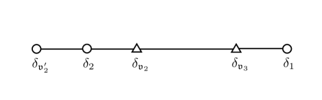
It still contains a codimension-one singularity at $(x_{1},y_{1},z,w)=(0,0,0,w)$ , which we call ${\mathfrak{p}}_{1}$ . The exceptional sets $C^{\pm}_{1}$ aligned over the curve ${\mathfrak{p}}_{0}$ are obtained by setting $z=0$ in (51) and the exceptional curve $\delta_{1}$ above the $E_{6}$ point are given by taking their $w\rightarrow 0$ limit (Figure 1):

\begin{cases}C^{+}_{1}\,:\,z=0,\,\,y_{1}=0\\ C^{-}_{1}\,:\,z=0,\,\,y_{1}=-wx_{1}\end{cases}\quad\rightarrow\quad\delta_{1}\,:\,w=0,\,\,z=0,\,\,y_{1}=0.

(52)

Blow up of ${\mathfrak{p}}_{1}$

To blow up ${\mathfrak{p}}_{1}$ , we set $(x_{1},y_{1},z)=(x_{1},x_{1}y_{2},x_{1}z_{2})$ as in (29). The geometric data after this blow up are given as follows:

\begin{split}&\Phi_{zx}\equiv x_{1}^{-2}\Phi_{z}=-y_{2}\{y_{2}+(w+a_{3,2}z_{2})\}+x_{1}z_{2}(x_{1}+w\,c+a_{4,3}z_{2}+a_{6,5}z_{2}^{2})=0.\\ &\mbox{Singularity}\,:\,{\mathfrak{v}}_{2}=(0,0,0,0),\\ &\begin{cases}C_{2}^{+}\,:\,x_{1}=0,\,\,y_{2}=0\\ C_{2}^{-}\,:\,x_{1}=0,\,\,y_{2}=-(w+a_{3,2}z_{2})\end{cases}\rightarrow\hskip 5.69046pt\begin{cases}\delta_{2}^{+}\,:\,x_{1}=0,\,\,y_{2}=0,\,\,w=0\\ \delta_{2}^{-}\,:\,x_{1}=0,\,\,y_{2}=-a_{3,2}z_{2},\,\,w=0\end{cases}\\ &\begin{cases}C_{1}^{+}\,:\,z_{2}=0,\,\,y_{2}=0\\ C_{1}^{-}\,:\,z_{2}=0,\,\,y_{2}=-w\end{cases}\hskip 82.51282pt\hskip 11.38092pt\delta_{1}\,:\,z_{2}=0,\,y_{2}=0,\,w=0.\end{split}

(53)

Here $C_{2}^{\pm}$ are the exceptional sets at generic $w$ arised via the blow up of $\mathfrak{p}_{1}$ and $\delta_{2}^{\pm}$ are their $w\rightarrow 0$ limits. $C_{1}^{\pm}$ and $\delta_{1}$ are the lift-ups of the objects defined in (52).

Refer to caption — Figure 1: The resolution process of the incomplete $E_{6}$ . ${\mathfrak{p}}_{1}$ is a codimension-one singularity; ${\mathfrak{v}}_{2}$ and ${\mathfrak{v}}_{3}$ are codimension-two singularities. The down arrows denote the limit $w\rightarrow 0$ . (For the complete case, one more codimension-two singularity ${\mathfrak{v}}_{4}$ remains. See section 4.2.2.)

The intersections of these objects are depicted in the second column of Figure 1. $C^{\pm}_{i}$ ’s form the $SU(5)$ Dynkin diagram. Three $\delta$ ’s meet at one point, where the singularity ${\mathfrak{v}}_{2}$ is located. This ${\mathfrak{v}}_{2}$ is not a conifold singularity since the second term of $\Phi_{zx}$ is of order three or higher. This type of singularities are known as generalized conifold singularities generalizedconifoldsingularities1 ; generalizedconifoldsingularities2 . Although it is not an ordinary conifold singularity, it can be regarded as consisting of two overlapping conifold singularities, which can be resolved by inserting two $\hbox{\mybb P}^{1}$ ’s successively as we will see below.

For this, we rewrite $\Phi_{zx}$ as we did in (32) as

\Phi_{zx}(u_{1},u_{2},u_{3},v_{1})=u_{1}u_{2}u_{3}-v_{1}\{v_{1}+(w+a_{3,2}u_{2})\}.

(54)

with

\begin{split}u_{1}&\equiv x_{1},\\ u_{2}&\equiv z_{2},\\ u_{3}&\equiv x_{1}+w\,c+a_{4,3}z_{2}+a_{6,5}z_{2}^{2},\\ v_{1}&\equiv y_{2}.\end{split}

(55)

$w$ in the second term of (54) is written using these coordinates as

w=\frac{1}{c}(u_{3}-u_{1}-a_{4,3}u_{2}-a_{6,5}u_{2}^{2}).

(56)

In the four-dimensional case, the corresponding geometry has the form $u_{1}u_{2}u_{3}-v_{1}v_{2}=0$ and the five coordinates are all independent, whereas in the six-dimensional case the coordinate $v_{2}$ is not independent.

The exceptional sets (53) are written in these coordinates as

\begin{split}&\begin{cases}\displaystyle C_{1}^{+}\,:\,u_{2}=0,\ v_{1}=0,\,w=\frac{1}{c}(u_{3}-u_{1}),\\ \displaystyle C_{1}^{-}\,:\,u_{2}=0,\,v_{1}=-w,\,w=\frac{1}{c}(u_{3}-u_{1}),\end{cases}\hskip 17.07182pt\delta_{1}\,:\,u_{2}=0,\,v_{1}=0,\,u_{3}=u_{1},\\ &\begin{cases}\displaystyle C_{2}^{+}\,:\,u_{1}=0,\,v_{1}=0,\,w=\frac{1}{c}(u_{3}-a_{4,3}u_{2}-a_{6,5}u_{2}^{2}),\,\\ \displaystyle C_{2}^{-}\,:\,u_{1}=0,\,v_{1}=-(w+a_{3,2}u_{2}),\,w=\frac{1}{c}(u_{3}-a_{4,3}u_{2}-a_{6,5}u_{2}^{2}),\,\end{cases}\\ &\hskip 113.81102pt\rightarrow\hskip 5.69046pt\begin{cases}\delta_{2}^{+}\,:\,u_{1}=0,\,v_{1}=0,\,u_{3}=a_{4,3}u_{2}+a_{6,5}u_{2}^{2},\,\\ \delta_{2}^{-}\,:\,u_{1}=0,\,v_{1}=-a_{3,2}u_{2},\,u_{3}=a_{4,3}u_{2}+a_{6,5}u_{2}^{2}.\end{cases}\end{split}

(57)

Resolution of ${\mathfrak{v}}_{2}$

For the first step of our resolution, we first insert $\hbox{\mybb P}^{1}$ in the $(u_{1},v_{1})$ plane as

(u_{1},v_{1})\equiv(\xi U_{1},\xi V_{1})

(58)

similarly to the Esole-Yau. There are two local coordinate patches: $U_{1}=1$ and $V_{1}=1$ , which we call patch $1$ and patch $2$ , respectively. In patch $1$ ,

(u_{1},v_{1})=(\xi,\xi V_{1}).

(59)

The resolved geometry is given by

\Phi_{zx1}(\xi,u_{2},u_{3},V_{1})\equiv\xi^{-1}\Phi_{zx}(\xi,u_{2},u_{3},\xi V_{1})=u_{2}u_{3}-V_{1}(\xi V_{1}+w+a_{3,2}u_{2})=0

(60)

with

w=\frac{1}{c}(u_{3}-\xi-a_{4,3}u_{2}-a_{6,5}u_{2}^{2}).

(61)

It contains a residual codimension-two singularity at the origin which we call ${\mathfrak{v}}_{3}$ :

{\mathfrak{v}}_{3}=(0,0,0,0).

(62)

The inserted $\hbox{\mybb P}^{1}$ (denoted as $\delta_{{\mathfrak{v}}_{2}}$ ) corresponds to the original singularity ${\mathfrak{v}}_{2}=(u_{1},u_{2},u_{3},v_{1})=(0,0,0,0)$ . In this patch, it is

\delta_{{\mathfrak{v}}_{2}}\,:\,\xi=0,\,u_{2}=0,\,u_{3}=0.

(63)

The exceptional sets (57) are now given by

\begin{split}&\begin{cases}\displaystyle C_{1}^{+}\,:\,u_{2}=0,\,V_{1}=0,\,w=\frac{1}{c}(u_{3}-\xi),\\ \displaystyle C_{1}^{-}\,:\,u_{2}=0,\,\xi V_{1}=-w,\,w=\frac{1}{c}(u_{3}-\xi),\end{cases}\hskip 14.22636pt\hskip 5.69046pt\delta_{1}\,:\,u_{2}=0,\,V_{1}=0,\,u_{3}=\xi,\\ &\begin{cases}\displaystyle C_{2}^{+}\,:\,\xi=0,\,u_{2}u_{3}=V_{1}(w+a_{3,2}u_{2}),\,w=\frac{1}{c}(u_{3}-a_{4,3}u_{2}-a_{6,5}u_{2}^{2}),\\ \displaystyle C_{2}^{-}\,:\,\mbox{invisible},\end{cases}\\ &\hskip 142.26378pt\begin{cases}\delta_{2}^{+}\,:\,\xi=0,\,u_{3}=a_{3,2}V_{1},\,u_{3}=a_{4,3}u_{2}+a_{6,5}u_{2}^{2},\\ \delta_{2}^{-}\,:\,\mbox{invisible}.\end{cases}\end{split}

(64)

Three exceptional curves $\delta_{{\mathfrak{v}}_{2}}$ , $\delta_{1}$ and $\delta_{2}^{+}$ are intersecting each other at one point and ${\mathfrak{v}}_{3}$ is located there (see the third diagram in the lower row in Figure 1)¹²¹²12The equations (64) are derived by substituting (59) into (57) and picking up the multiplicity-one independent component in $\Phi_{zx1}=0$ . For $C_{1}^{+}$ , the substitution gives the form $u_{2}=0,\,\,\,\xi V_{1}=0,\,\,\,w=\frac{1}{c}(u_{3}-\xi).$ Since this $C_{1}^{+}$ is a subvariety of $\Phi_{zx1}=0$ , an additional constraint $V_{1}w=0$ should be satisfied. It is solved by $V_{1}=0$ since $w\neq 0$ at generic point of the codimension-one discriminant locus. Then the second equation $\xi V_{1}=0$ is satisfied, giving the form of $C_{1}^{+}$ in (64). Also, $\delta_{1}$ is rewritten as $u_{2}=0,\,\,\,\xi V_{1}=0,\,\,\,u_{3}=\xi,$ which satisfies $\Phi_{zx1}=0$ . It has two components $u_{2}=0,\xi=0,u_{3}=0$ and $u_{2}=0,V_{1}=0,u_{3}=\xi$ . The former one is equivalent to $\delta_{{\mathfrak{v}}_{2}}$ (63), and hence the latter component gives the equation of $\delta_{1}$ . The forms of $C_{1}^{-}$ , $C_{2}^{+}$ and $\delta_{2}^{+}$ are similarly obtained. $C_{2}^{-}$ is given by the equations $\xi=0,\,\,\,0=-(w+a_{3,2}u_{2}),\,\,\,w=\frac{1}{c}(u_{3}-a_{4,3}u_{2}-a_{6,5}u_{2}^{2}),\,\,\,u_{2}u_{3}=0,$ where the last condition comes from $\Phi_{zx1}=0$ . From the second equation, $u_{2}\neq 0$ for generic $w$ , and hence $u_{3}=0$ from the last equation. The second and the third equations yield $w=-a_{3,2}u_{2}$ and $-c\,a_{3,2}+a_{4,3}+a_{6,5}u_{2}=0$ , which have no solution for generic $w$ . Thus $C_{2}^{-}$ is invisible in this patch. The equation of $\delta_{2}^{-}$ is equivalent to $\delta_{{\mathfrak{v}}_{2}}$ and has no independent component..

Naïvely, one might think of $\delta_{1}$ as arising from $C_{1}^{+}$ and $C_{1}^{-}$ , or $\delta_{\mathscr{v}_{2}}$ as from $C_{2}^{+}$ and $C_{2}^{-}$ only. In fact, however, if one carefully examines how the defining equations of these exceptional sets factorize in the $w\rightarrow 0$ limit, one can recognize exactly which exceptional sets that occur in the limit are composed of which exceptional sets defined prior to taking the limit MT ; Yukawas ; halfhyper . For example, from (64), one can see that the limit $w\rightarrow 0$ of $C$ ’s are written in terms of $\delta$ ’s as follows:

C_{1}^{+}\rightarrow\delta_{1},\quad C_{1}^{-}\rightarrow\delta_{1}+\delta_{{\mathfrak{v}}_{2}},\quad C_{2}^{+}\rightarrow\delta_{2}^{+}+\delta_{{\mathfrak{v}}_{2}}.

(65)

The limit of $C_{2}^{+}$ is obtained by

\begin{split}\mbox{lim}_{w\rightarrow 0}\,C_{2}^{+}&=\{\xi=0,\,u_{2}u_{3}=V_{1}a_{3,2}u_{2},\,u_{3}=a_{4,3}u_{2}+a_{6,5}u_{2}^{2}\}\\ &=\{\xi=0,\,u_{3}=V_{1}a_{3,2},\,u_{3}=a_{4,3}u_{2}+a_{6,5}u_{2}^{2}\}\cup\{\xi=0,\,u_{2}=0,\,u_{3}=0\}\\ &=\delta_{2}^{+}\cup\delta_{{\mathfrak{v}}_{2}}.\end{split}

(66)

Similar calculations will be done repeatedly throughout this paper. Note that the summations in (65) should be understood as those in the weight space of $SU(5)$ or divisors Yukawas .

In the other patch $(u_{1},v_{1})=(\xi U_{1},\xi)$ (patch 2, the $V_{1}=1$ patch), the resolved geometry is given by

\begin{split}\Phi_{zx2}(U_{1},u_{2},u_{3},\xi)&\equiv\xi^{-1}\Phi_{zx}(\xi U_{1},u_{2},u_{3},\xi)=U_{1}u_{2}u_{3}-(\xi+w+a_{3,2}u_{2})=0,\\ &w=\frac{1}{c}\big{\{}u_{3}-\xi U_{1}-a_{4,3}u_{2}-a_{6,5}u_{2}^{2}\big{\}}.\end{split}

(67)

It contains no singularity and is regular. The intersections and limits are similarly calculated as in patch $1$ (the $U_{1}=1$ patch). We found that $\delta_{2}^{-}\cdot\delta_{{\mathfrak{v}}_{2}}\neq 0$ and ( $C_{1}^{+}$ and $\delta_{1}$ are invisible)

C_{1}^{-}\rightarrow\delta_{{\mathfrak{v}}_{2}},\quad C_{2}^{+}\rightarrow\delta_{2}^{+}+\delta_{{\mathfrak{v}}_{2}},\quad C_{2}^{-}\rightarrow\delta_{2}^{-}.

(68)

This completes the first step of our small resolution. The result is summarized in the third diagram in the lower row of Figure 1.

The remaining codimension-two singularity ${\mathfrak{v}}_{3}$ in patch $1$ (the $U_{1}=1$ patch) is a conifold singularity since $\Phi_{zx1}$ (60) has the form

\Phi_{zx1}(\xi,u_{2},u_{3},V_{1})=u_{2}u_{3}-V_{1}\{w+\cdots\}=u_{2}u_{3}-V_{1}\big{\{}-\frac{1}{c}\xi+\cdots\big{\}}.

(69)

It is resolved by a standard small resolution, which is the second step of our resolution. This means that ${\mathfrak{v}}_{2}$ consists of two overlapping conifold singularities.

Resolution of ${\mathfrak{v}}_{3}$

For this small resolution, we choose the plane $(u_{3},V_{1})$ and insert a $\hbox{\mybb P}^{1}$ (denoted as $\delta_{{\mathfrak{v}}_{3}}$ ) as follows :

(u_{3},V_{1})=(\eta U_{3},\eta V^{\prime}_{1}).

(70)

The two patches with $U_{3}=1$ and $V^{\prime}_{1}=1$ are denoted as patch $1^{\prime}$ and patch $2^{\prime}$ . In patch $1^{\prime}$ with $(u_{3},V_{1})=(\eta,\eta V^{\prime}_{1})$ , the data of the resolved geometry is given by

\begin{split}&\Phi_{zx11^{\prime}}(\xi,u_{2},\eta,V^{\prime}_{1})\equiv\eta^{-1}\Phi_{zx1}(\xi,u_{2},\eta,\eta V^{\prime}_{1})=u_{2}-V^{\prime}_{1}(\xi\eta V^{\prime}_{1}+w+a_{3,2}u_{2})=0,\\ &\hskip 76.82234ptw=\frac{1}{c}(\eta-\xi-a_{4,3}u_{2}-a_{6,5}u_{2}^{2}).\\ &\mbox{Singularity : none (regular)},\\ &\begin{cases}\displaystyle C_{1}^{+}\,:\,u_{2}=0,\,V^{\prime}_{1}=0,\,w=\frac{1}{c}(\eta-\xi),\\ \displaystyle C_{1}^{-}\,:\,u_{2}=0,\,\xi\eta V^{\prime}_{1}=-w,\,w=\frac{1}{c}(\eta-\xi),\end{cases}\hskip 42.67912pt\delta_{1}\,:\,\,u_{2}=0,V^{\prime}_{1}=0,\,\eta=\xi,\\ &\hskip 11.38092ptC_{2}^{+}\,:\,\xi=0,\,u_{2}=V^{\prime}_{1}(w+a_{3,2}u_{2}),\,w=\frac{1}{c}(\eta-a_{4,3}u_{2}-a_{6,5}u_{2}^{2}),\\ &\hskip 184.9429pt\delta_{2}^{+}\,:\,\xi=0,\,a_{3,2}V^{\prime}_{1}=1,\,\eta=a_{4,3}u_{2}+a_{6,5}u_{2}^{2},\\ &\hskip 184.9429pt\delta_{{\mathfrak{v}}_{2}}\,:\,\mbox{invisible},\\ &\hskip 184.9429pt\delta_{{\mathfrak{v}}_{3}}\,:\,\xi=0,\,\eta=0,u_{2}=0.\end{split}

(71)

$\delta_{1}$ and $\delta_{{\mathfrak{v}}_{3}}$ intersect at the origin, whereas $\delta_{2}^{+}$ and $\delta_{{\mathfrak{v}}_{3}}$ intersect at another point $(\xi,u_{2},\eta,V^{\prime}_{1})=(0,0,0,\frac{1}{a_{3,2}})$ :

\delta_{1}\cdot\delta_{{\mathfrak{v}}_{3}}\neq 0,\quad\delta_{2}^{+}\cdot\delta_{{\mathfrak{v}}_{3}}\neq 0.

(72)

The limits can be read from (71) as

C_{1}^{+}\rightarrow\delta_{1},\quad C_{1}^{-}\rightarrow\delta_{1}+2\delta_{{\mathfrak{v}}_{3}},\quad C_{2}^{+}\rightarrow\delta_{2}^{+}+\delta_{{\mathfrak{v}}_{3}}.

(73)

For example,

\begin{split}\mbox{lim}_{w\rightarrow 0}\,C_{1}^{-}&=\{u_{2}=0,\,\xi\eta V^{\prime}_{1}=0,\,0=\eta-\xi\}\\ &=\{u_{2}=0,\,\eta^{2}V^{\prime}_{1}=0,\xi=\eta\}\\ &=\{u_{2}=0,\,V^{\prime}_{1}=0,\,\xi=\eta\}\cup\{u_{2}=0,\,\eta=0,\,\xi=0\}^{\otimes 2}\\ &=\delta_{1}\cup 2\delta_{{\mathfrak{v}}_{3}}.\end{split}

(74)

In patch $2^{\prime}$ with $(u_{3},V_{1})=(\eta U_{3},\eta)$ (the $V^{\prime}_{1}=1$ patch), the resolved geometry is given by

\begin{split}&\Phi_{zx12^{\prime}}(\xi,u_{2},U_{3},\eta)\equiv\eta^{-1}\Phi_{zx1}(\xi,u_{2},\eta U_{3},\eta)=u_{2}U_{3}-(\xi\eta+w+a_{3,2}u_{2})=0,\\ &\hskip 76.82234ptw=\frac{1}{c}(\eta U_{3}-\xi-a_{4,3}u_{2}-a_{6,5}u_{2}^{2}).\end{split}

(75)

These equations are the same as (47) and (48) with $a_{1,0}=w$ and $a_{2,1}=wc$ substituted. $\Phi_{zx12^{\prime}}$ is denoted by $\Phi_{zx\xi\eta}$ in (47)¹³¹³13 The constraint is solved for $w$ here, whereas it is (formally) solved for $\xi$ in (48). Of cource the geometry is the same.. The other geometric data are given by

\begin{split}&\hskip 11.38092pt\mbox{Singularity\,:\, none (regular)},\\ &\begin{cases}\displaystyle C_{1}^{+}\,:\,\mbox{invisible},\\ \displaystyle C_{1}^{-}\,:\,u_{2}=0,\,\xi\eta=-w,\,w=\frac{1}{c}(\eta U_{3}-\xi),\end{cases}\hskip 14.22636pt\hskip 62.59596pt\delta_{1}\,:\,\mbox{invisible},\\ &\hskip 11.38092ptC_{2}^{+}\,:\,\xi=0,\,u_{2}U_{3}=(w+a_{3,2}u_{2}),\,w=\frac{1}{c}(\eta U_{3}-a_{4,3}u_{2}-a_{6,5}u_{2}^{2}),\\ &\hskip 156.49014pt\delta_{2}^{+}\,:\,\xi=0,\,U_{3}=a_{3,2},\,\eta U_{3}=a_{4,3}u_{2}+a_{6,5}u_{2}^{2},\\ &\hskip 156.49014pt\delta_{{\mathfrak{v}}_{2}}\,:\,\xi=0,\,u_{2}=0,\,U_{3}=0,\\ &\hskip 156.49014pt\delta_{{\mathfrak{v}}_{3}}\,:\,\xi=0,\,u_{2}=0,\,\eta=0.\end{split}

(76)

$\delta_{2}^{+}$ and $\delta_{{\mathfrak{v}}_{3}}$ intersect at $(\xi,u_{2},U_{3},\eta)=(0,0,a_{3,2},0)$ , whereas $\delta_{{\mathfrak{v}}_{2}}$ and $\delta_{{\mathfrak{v}}_{3}}$ intersect at the origin:

\delta_{2}^{+}\cdot\delta_{{\mathfrak{v}}_{3}}\neq 0,\quad\delta_{{\mathfrak{v}}_{2}}\cdot\delta_{{\mathfrak{v}}_{3}}\neq 0.

(77)

The limits are given by

C_{1}^{-}\rightarrow\delta_{{\mathfrak{v}}_{2}}+2\delta_{{\mathfrak{v}}_{3}},\quad C_{2}^{+}\rightarrow\delta_{2}^{+}+\delta_{{\mathfrak{v}}_{2}}+\delta_{{\mathfrak{v}}_{3}}.

(78)

This completes the resolution process. The whole intersecting pattern is shown in the rightmost diagram in Figure 1. The limits of $C_{i}$ ’s are obtained by taking the union of the results of all patches (65), (68), (73) and (78) as

\begin{split}C_{1}^{+}&=\delta_{1},\\ C_{1}^{-}&=\delta_{1}+\delta_{{\mathfrak{v}}_{2}}+2\delta_{{\mathfrak{v}}_{3}},\\ C_{2}^{+}&=\delta_{2}^{+}+\delta_{{\mathfrak{v}}_{2}}+\delta_{{\mathfrak{v}}_{3}},\\ C_{2}^{-}&=\delta_{2}^{-},\end{split}

(79)

where, again, the equalities should be understood as those of $SU(5)$ weights or divisors. Under this identification, one can easily check that the intersection matrix of $C_{i}$ ’s is equivalent to (minus) the $SU(5)$ Cartan matrix if the intersection matrix of $\delta_{i}$ ’s has the form

\delta_{i}\cdot\delta_{j}=-\left(\begin{array}[]{rrrrr}2&-1&0&0&0\\ -1&2&-1&0&0\\ 0&-1&\frac{3}{2}&-\frac{1}{2}&-1\\ 0&0&-\frac{1}{2}&\frac{3}{2}&0\\ 0&0&-1&0&2\end{array}\right),

(80)

where the rows and the columns are ordered as $\delta_{2}^{-},\delta_{{\mathfrak{v}}_{2}},\delta_{{\mathfrak{v}}_{3}},\delta_{2}^{+}$ and $\delta_{1}$ . This intersection matrix is depicted in Figure 2. The second node from the right of the $E_{6}$ Dynkin diagram is removed¹⁴¹⁴14 If we insert $\hbox{\mybbsub P}^{1}$ in the plane $(u_{2},V_{1})$ instead of the plane $(u_{3},V_{1})$ (70) in the second step of the resolution, the intersection matrix is the one that the center node of the $E_{6}$ Dynkin diagram is removed. .

Let us now define curves $J$ above the incomplete $E_{6}$ point as linear combinations of $\delta$ ’s with integer coefficients via

J\equiv\sum_{n_{i}}n_{i}\delta_{i}\quad\mbox{with}\quad n_{i}\in\hbox{\mybb Z}.

(81)

The intersection matrix of $\delta$ ’s defines a lattice which is the projection of the root lattice of $E_{6}$ in the direction orthogonal to the root of the removed node. By this projection, the curves corresponding to the roots of $E_{6}$ , which have self intersection number $J.J=-2$ , are projected to the states with $-2\leq J.J<0$ (apart from $J.J=0$ ). It is shown that possible such self-intersections of $J$ are $-2$ or $-\frac{3}{2}$ and the numbers of such curves are $30$ or $20$ , respectively. These curves can be thought of as forming a representation of a charged matter hypermultiplet. Former curves are “adjoint of incomplete $E_{6}$ ” and taking their coset by $SU(5)$ gives $\mathbb{5}$ , while the latter curves form $\mathbb{10}$ :

\begin{split}&\sharp(J.J=-2)=30\rightarrow\mathbb{5},\\ &\sharp(J.J=-\frac{3}{2})=20\rightarrow\mathbb{10}.\end{split}

(82)

In conclusion, an incomplete $E_{6}$ singularity gives matter multiplet $\mathbb{10}\oplus\mathbb{5}$ , which is nothing but the expected result from the anomaly-free condition. Recall that $o_{w}(a_{1,0})=1$ and $o_{w}(P_{8,5})=1$ for the incomplete $E_{6}$ (see Table 2).

4.2.2 Complete $E_{6}$

Next let us move on to the complete $E_{6}$ geometry. Since
$(\mbox{o}_{w}(a_{1,0}),\mbox{o}_{w}(a_{2,1}),\mbox{o}_{w}(a_{3,2}),\mbox{o}_{w}(a_{4,3}),\mbox{o}_{w}(a_{6,5}),\mbox{o}_{w}(P_{8,5}))=(2,1,0,0,0,1)$ are the conditions for a complete $E_{6}$ singularity, we set

\begin{split}a_{1,0}&=w^{2},\\ a_{2,1}&=w\,c.\end{split}

(83)

The equation (27) of this geometry is given by

\Phi\equiv-(y^{2}+\underline{w^{2}}xy+a_{3,2}z^{2}y)+x^{3}+w\,c\,zx^{2}+a_{4,3}z^{3}x+a_{6,5}z^{5}=0.

(84)

It differs from the incomplete case in the underlined term.

The first and second resolutions of codimension-one singularities proceed in the same manner as was done in the incomplete case. The geometry after the resolution of ${\mathfrak{p}}_{1}$ is similar to the incomplete case (54) and has the form

\Phi_{zx}=u_{1}u_{2}u_{3}-v_{1}\{v_{1}+(\underline{w^{2}}+a_{3,2}u_{2})\}=0,

(85)

where the only difference is the underlined term. The definition of the coordinates $u_{1}$ , $u_{2}$ , $u_{3}$ and $v_{1}$ are the same as (55). Also, $w$ is the same as (56). The geometry contains a generalized conifold singularity ${\mathfrak{v}}_{2}$ (see the second column of Figure 1).

Resolution of ${\mathfrak{v}}_{2}$

The resolution of ${\mathfrak{v}}_{2}$ is done in parallel with the incomplete case. The resulting intersections of $C$ ’s and $\delta$ ’s are the same as the incomplete case (the third diagram in the lower row of Figure 1). The limits of $C$ ’s are also the same as (65) and (68).

A difference arises in the property of the remaining singularity ${\mathfrak{v}}_{3}$ which resides at the origin $(\xi,u_{2},u_{3},V_{1})=(0,0,0,0)$ in patch $1$ (59). In the incomplete case, ${\mathfrak{v}}_{3}$ is a conifold singularity as seen in (60) and (69). On the other hand, in the complete case, ${\mathfrak{v}}_{3}$ is not a conifold singularity, since the resolved geometry is given by

\begin{split}\Phi_{zx1}(\xi,u_{2},u_{3},V_{1})&=u_{2}u_{3}-V_{1}\{\xi V_{1}+(\underline{w^{2}}+a_{3,2}u_{2})\}=0,\\ w&=\frac{1}{c}(u_{3}-\xi-a_{4,3}u_{2}-a_{6,5}u_{2}^{2}),\end{split}

(86)

which is not a conifold: the underlined part $-V_{1}w^{2}$ is now cubic. Also, it does not look like a generalized conifold singularity form, since the cubic terms do not seem to be factorizable. However, as we will see below, at least at special points of the complex moduli space, it does have the generalized conifold singularity form and the singularity ${\mathfrak{v}}_{3}$ is resolved by inserting two $\hbox{\mybb P}^{1}$ ’s. In other words, ${\mathfrak{v}}_{2}$ is an singularity where the three conifold singularities overlap.

The exceptional sets in this patch are given by appropriately replacing $w$ with $w^{2}$ in the incomplete ones (63) and (64) (underlined terms):

\begin{split}&\begin{cases}\displaystyle C_{1}^{+}\,:\,u_{2}=0,\,V_{1}=0,\,w=\frac{1}{c}(u_{3}-\xi),\\ \displaystyle C_{1}^{-}\,:\,u_{2}=0,\,\xi V_{1}=-\underline{w^{2}},\,w=\frac{1}{c}(u_{3}-\xi),\end{cases}\hskip 14.22636pt\hskip 8.5359pt\delta_{1}\,:\,u_{2}=0,\,V_{1}=0,\,u_{3}=\xi,\\ &\begin{cases}\displaystyle C_{2}^{+}\,:\,\xi=0,\,u_{2}u_{3}=V_{1}(\underline{w^{2}}+a_{3,2}u_{2}),\,w=\frac{1}{c}(u_{3}-a_{4,3}u_{2}-a_{6,5}u_{2}^{2}),\\ \displaystyle C_{2}^{-}\,:\,\mbox{invisible},\end{cases}\\ &\hskip 150.79968pt\begin{cases}\delta_{2}^{+}\,:\,\xi=0,\,u_{3}=a_{3,2}V_{1},\,u_{3}=a_{4,3}u_{2}+a_{6,5}u_{2}^{2},\\ \delta_{2}^{-}\,:\,\mbox{invisible}.\end{cases}\\ &\hskip 159.3356pt\,\delta_{{\mathfrak{v}}_{2}}\,:\,\xi=0,\,u_{2}=0,\,u_{3}=0.\end{split}

(87)

Resolution of ${\mathfrak{v}}_{3}$

Let us try to resolve ${\mathfrak{v}}_{3}$ by inserting $\hbox{\mybb P}^{1}$ in the plane $(u_{3},V_{1})$ as before. In patch $1^{\prime}$ , where $(u_{3},V_{1})=(\eta,\eta V^{\prime}_{1})$ , we obtain a regular geometry. The intersections and limits are the same as those in the incomplete case (72) and (73). On the other hand, in patch $2^{\prime}$ with $(u_{3},V_{1})=(\eta U_{3},\eta)$ , the resolved geometry still contains a codimension-two singularity ${\mathfrak{v}}_{4}$ . Replacing $w$ with $w^{2}$ in (75), we have

\begin{split}&\Phi_{zx12^{\prime}}(\xi,u_{2},U_{3},\eta)=u_{2}U_{3}-\{\xi\eta+(\underline{w^{2}}+a_{3,2}u_{2})\}=0,\\ &w=\frac{1}{c}(\eta U_{3}-\xi-a_{4,3}u_{2}-a_{6,5}u_{2}^{2}).\\ &\mbox{Singularity : }\,{\mathfrak{v}}_{4}=(0,0,a_{3,2},0).\end{split}

(88)

After the coordinate shift

\widetilde{U}_{3}\equiv U_{3}-a_{3,2},

(89)

the resolved geometry is given by

\begin{split}&\Phi_{zx12^{\prime}}(\xi,u_{2},\widetilde{U}_{3},\eta)=u_{2}\widetilde{U}_{3}-\{\xi\eta+w^{2}\}=0,\\ &w=\frac{1}{c}(\eta\widetilde{U}_{3}+a_{3,2}\eta-\xi-a_{4,3}u_{2}-a_{6,5}u_{2}^{2}),\end{split}

(90)

where ${\mathfrak{v}}_{4}$ is now located at the origin. In general, it does not have a conifold form because of the subleading terms, but at a special point of the complex moduli space

a_{4,3}=a_{6,5}=0,

(91)

$\Phi_{zx12^{\prime}}$ is decomposed into the part proportional to $\widetilde{U}_{3}$ and the remaining part of quadratic in $\xi$ and $\eta$ , and then the geometry is in a conifold form and ${\mathfrak{v}}_{4}$ is a conifold singularity. Explicitly, one can write

\Phi_{zx12^{\prime}}=\tilde{u}_{2}\widetilde{U}_{3}-\zeta_{+}\zeta_{-}=0,

(92)

where the coordinates $\tilde{u}_{2}$ and $\zeta_{\pm}$ are defined by

\begin{split}\tilde{u}_{2}&\equiv u_{2}-\frac{1}{c^{2}}\{2\eta(a_{3,2}\eta-\xi)+\eta^{2}\widetilde{U}_{3}\},\\ \zeta_{\pm}&\equiv\frac{1}{c}(\xi+\alpha_{\pm}\eta)\end{split}

(93)

with

\alpha_{+}+\alpha_{-}=-2a_{3,2}+c^{2}\,,\quad\quad\alpha_{+}\alpha_{-}=a_{3,2}^{2}.

(94)

Going back to the geometry $\Phi_{zx1}=0$ (86), it exactly has the generalized conifold form under the specializations (91), so that

\Phi_{zx1}=\tilde{u}_{2}\tilde{u}_{3}-\frac{1}{c^{2}}V_{1}(\xi+\alpha_{+}V_{1})(\xi+\alpha_{-}V_{1})=0,

(95)

where $\tilde{u}_{3}=u_{3}-a_{3,2}V_{1}$ and $\tilde{u}_{2}=u_{2}-\frac{V_{1}}{c^{2}}\{\tilde{u}_{3}+2(a_{3,2}V_{1}-\xi)\}$ .

It should be noted that the specializations (91) do not change the structure of $E_{6}$ singularity. For these specializations, though the order of $f$ enhances to $\infty$ at $w=0$ , the order of $g$ is kept to be $4$ since $a_{3,2}\neq 0$ (see (13) and Table 1). Also, all the intersections $C_{i}\cdot C_{j}$ , $\delta_{i}\cdot\delta_{j}$ and the limits $\mbox{lim}_{w\rightarrow 0}C_{i}$ are the same as the generic case¹⁵¹⁵15Only non-trivial difference is the definition of $\delta_{2}^{+}$ in patch $2^{\prime}$ in the second step of our resolution (76). It is modified to be $\delta_{2}^{+}\,:\,\xi=0,\,\eta=0,\,U_{3}=a_{3,2}$ . Nevertheless, the limit of $C_{2}^{+}$ is the same as (78). . Therefore, nothing changes even if we impose the condition (91) from the beginning.

The exceptional sets (87) are rewritten in the coordinates $(\widetilde{U}_{3},\tilde{u}_{2},\zeta_{+},\zeta_{-})$ as ( $C_{1}^{+}$ , $C_{2}^{-}$ , $\delta_{1}$ and $\delta_{2}^{-}$ are invisible in this patch)

\begin{split}&C_{1}^{-}\,:\,\tilde{u}_{2}=-\frac{1}{c^{2}}\eta\,\big{(}2c\,w-\eta\widetilde{U}_{3}\big{)},\,\xi\eta=-w^{2},\,w=\frac{1}{c}\{\eta(\widetilde{U}_{3}+a_{3,2})-\xi\},\\ &C_{2}^{+}\,:\,\alpha_{+}\zeta_{-}=\alpha_{-}\zeta_{+},\,\widetilde{U}_{3}\tilde{u}_{2}=\zeta_{+}\zeta_{-},\,w=\frac{1}{\alpha_{+}-\alpha_{-}}(\zeta_{+}-\zeta_{-})(\widetilde{U}_{3}+a_{3,2}),\\ &\delta_{2}^{+}\,:\,\zeta_{+}=0,\,\zeta_{-}=0,\,\widetilde{U}_{3}=0,\\ &\delta_{{\mathfrak{v}}_{2}}\,:\,\xi=0,\,\tilde{u}_{2}=-\frac{16}{c^{2}}a_{3,2}\eta^{2},\,\widetilde{U}_{3}=-a_{3,2},\\ &\delta_{{\mathfrak{v}}_{3}}\,:\,\zeta_{+}=0,\,\zeta_{-}=0,\,\tilde{u}_{2}=0,\end{split}

(96)

where $\xi$ and $\eta$ are written by $\zeta_{\pm}$ as

\xi=\frac{c}{\alpha_{+}-\alpha_{-}}(\alpha_{+}\zeta_{-}-\alpha_{-}\zeta_{+}),\quad\eta=\frac{c}{\alpha_{+}-\alpha_{-}}(\zeta_{+}-\zeta_{-}).

(97)

In particular, one can show that $\xi=0$ yields $\eta^{2}=\frac{c^{2}}{a_{3,2}^{2}}\zeta_{+}\zeta_{-}$ , which we used to obtain the form of $C_{2}^{+}$ in (96). The intersections and the limits of these objects are the same as those for the incomplete case (77) and (78). The conifold singularity ${\mathfrak{v}}_{4}$ is located at the intersection point of $\delta_{2}^{+}$ and $\delta_{{\mathfrak{v}}_{3}}$ as shown in the rightmost diagram in Figure 1.

Resolution of ${\mathfrak{v}}_{4}$

For the final step of the resolution process, let us resolve the conifold singularity ${\mathfrak{v}}_{4}$ (92) by inserting $\hbox{\mybb P}^{1}$ in $(\widetilde{U}_{3},\zeta_{+})$ plane as

(\widetilde{U}_{3},\zeta_{+})=(U^{\prime}_{3}\chi,Z_{+}\chi).

(98)

In the coordinate patch $(\widetilde{U}_{3},\zeta_{+})=(\chi,Z_{+}\chi)$ (denoted as patch $1^{\prime\prime}$ ), the resolved geometry is given by

\begin{split}&\Phi_{zx12^{\prime}1^{\prime\prime}}=\chi^{-1}\Phi_{zx12^{\prime}}=\tilde{u}_{2}-Z_{+}\zeta_{-}=0.\\ &\mbox{Singularity~{}:}\,\mbox{none (regular)},\\ &C_{1}^{-}\,:\,\tilde{u}_{2}=-\frac{1}{c^{2}}\eta\,\big{(}2c\,w-\eta\chi\big{)},\,\frac{\xi\eta+w^{2}}{\chi}=0,\,w=\frac{1}{c}\{\eta(\chi+a_{3,2})-\xi\},\\ &C_{2}^{+}\,:\,\alpha_{+}\zeta_{-}=\alpha_{-}Z_{+}\chi,\,\tilde{u}_{2}=Z_{+}\zeta_{-},\,w=\frac{1}{\alpha_{+}-\alpha_{-}}(Z_{+}\chi-\zeta_{-})(\chi+a_{3,2}),\\ &\delta_{2}^{+}\,:\,\mbox{invisible},\\ &\delta_{{\mathfrak{v}}_{2}}\,:\,\alpha_{+}\zeta_{-}=\alpha_{-}Z_{+}\chi,\,\tilde{u}_{2}=-\frac{a_{3,2}}{\alpha_{-}^{2}}\zeta_{-}^{2},\,\chi=-a_{3,2},\\ &\delta_{{\mathfrak{v}}_{3}}\,:\,Z_{+}=0,\,\zeta_{-}=0,\,\tilde{u}_{2}=0,\\ &\delta_{{\mathfrak{v}}_{4}}\,:\,\chi=0,\,\zeta_{-}=0,\,\tilde{u}_{2}=0.\end{split}

(99)

The intersections are

\delta_{{\mathfrak{v}}_{2}}\cdot\delta_{{\mathfrak{v}}_{3}}\neq 0,\quad\delta_{{\mathfrak{v}}_{3}}\cdot\delta_{{\mathfrak{v}}_{4}}\neq 0.

(100)

Let us explain how the second equation of $C_{1}^{-}$ is obtained. In the previous patch, it has the form $\xi\eta+w^{2}=0$ (96). It is rewritten in the present patch as

\begin{split}\xi\eta+w^{2}&\sim c^{2}(\alpha_{+}\zeta_{-}-\alpha_{-}Z_{+}\chi)(Z_{+}\chi-\zeta_{-})+\big{\{}(Z_{+}\chi-\zeta_{-})(\chi+a_{3,2})-(\alpha_{+}\zeta_{-}-\alpha_{-}Z_{+}\chi)\big{\}}^{2}\\ &=\zeta_{-}^{2}\big{\{}-c^{2}\alpha_{+}+(a_{3,2}+\alpha_{+})^{2}\big{\}}+\chi\{\cdots\}\\ &=\chi\{\cdots\}.\end{split}

Here the coefficient of $\zeta_{-}^{2}$ vanishes because of (94). Thus $C_{1}^{-}$ contains the component with $\chi=0$ . It is easily seen that this component is not complex one dimensional but merely a point. In order to subtract this irrelevant component, the second equation is divided by $\chi$ .

Let us evaluate the limit $w\rightarrow 0$ of $C_{1}^{-}$ in the present patch. Firstly, we estimate the third equation of $C_{1}^{-}$ (99) at $w=0$ . By substituting (97) and $(\widetilde{U}_{3},\zeta_{+})=(\chi,Z_{+}\chi)$ into the equation, we find that $\zeta_{-}$ is factorized by $\chi$ as

(\alpha_{+}+a_{3,2})\zeta_{-}=\chi\{Z_{+}(\alpha_{-}+a_{3,2}+\chi)-\zeta_{-}\}.

(101)

Then, $\xi$ (97) is also factorized by $\chi$ such that

\begin{split}(\alpha_{+}+a_{3,2})\xi&\sim(\alpha_{+}+a_{3,2})(\alpha_{+}\zeta_{-}-\alpha_{-}Z_{+}\chi)\\ &=\chi\big{[}\alpha_{+}\{Z_{+}(\alpha_{-}+a_{3,2}+\chi)-\zeta_{-}\}-(\alpha_{+}+a_{3,2})\alpha_{-}Z_{+}\big{]}\\ &=\chi\alpha_{+}\big{\{}Z_{+}(a_{3,2}\frac{\alpha_{+}-\alpha_{-}}{\alpha_{+}}+\chi)-\zeta_{-}\big{\}}.\end{split}

(102)

Thus the second equation of $C_{1}^{-}$ is estimated at $w=0$ as

\frac{\xi\eta}{\chi}\sim\big{\{}Z_{+}(a_{3,2}\frac{\alpha_{+}-\alpha_{-}}{\alpha_{+}}+\chi)-\zeta_{-}\big{\}}(Z_{+}\chi-\zeta_{-})=0.

(103)

Plugging back one of its solution $\zeta_{-}=Z_{+}(a_{3,2}\frac{\alpha_{+}-\alpha_{-}}{\alpha_{+}}+\chi)$ into the third equation (101), we obtain a simple form

Z_{+}(\chi+a_{3,2})=0.

(104)

Also, substituting the other solution $\zeta_{-}=Z_{+}\chi$ into (101), we have

Z_{+}\chi=0.

(105)

Therefore,

\begin{split}\mbox{lim}_{w\rightarrow 0}\,C_{1}^{-}&=\{\tilde{u}_{2}=\frac{1}{c^{2}}\eta^{2}\chi,\,\zeta_{-}=Z_{+}(a_{3,2}\frac{\alpha_{+}-\alpha_{-}}{\alpha_{+}}+\chi),\,Z_{+}(\chi+a_{3,2})=0\}\\ &\quad\cup\{\tilde{u}_{2}=\frac{1}{c^{2}}\eta^{2}\chi,\,\zeta_{-}=Z_{+}\chi,\,Z_{+}\chi=0\}\\ &=\{Z_{+}=0,\,\zeta_{-}=0,\,\tilde{u}_{2}=0\}\cup\{\chi=-a_{3,2},\,\zeta_{-}=-Z_{+}a_{3,2}\frac{\alpha_{-}}{\alpha_{+}},\,\tilde{u}_{2}=-\frac{1}{c^{2}}\eta^{2}a_{3,2}\}\\ &\quad\cup\{Z_{+}=0,\,\zeta_{-}=0,\,\tilde{u}_{2}=0\}\cup\{\chi=0,\,\zeta_{-}=0,\,\tilde{u}_{2}=0\}\\ &=\delta_{{\mathfrak{v}}_{2}}\cup 2\delta_{{\mathfrak{v}}_{3}}\cup\delta_{{\mathfrak{v}}_{4}}.\end{split}

(106)

The limit of $C_{2}^{+}$ (99) is easily calculated as

\begin{split}\mbox{lim}_{w\rightarrow 0}\,C_{2}^{+}&=\{\alpha_{+}\zeta_{-}=\alpha_{-}Z_{+}\chi,\,\tilde{u}_{2}=Z_{+}\zeta_{-},\,\zeta_{-}=Z_{+}\chi\}\\ &\quad\cup\{\alpha_{+}\zeta_{-}=\alpha_{-}Z_{+}\chi,\,\tilde{u}_{2}=Z_{+}\zeta_{-},\,\chi=-a_{3,2}\}\\ &=\{Z_{+}\chi=0,\,\zeta_{-}=0,\,\tilde{u}_{2}=0\}\cup\{\alpha_{+}\zeta_{-}=\alpha_{-}Z_{+}\chi,\,\tilde{u}_{2}=-\frac{\alpha_{+}}{a_{3,2}\alpha_{-}}\zeta_{-}^{2},\,\chi=-a_{3,2}\}\\ &=\delta_{{\mathfrak{v}}_{2}}\cup\delta_{{\mathfrak{v}}_{3}}\cup\delta_{{\mathfrak{v}}_{4}}.\end{split}

(107)

Compared with the incomplete case (79), one can see that both of the limit of $C_{1}^{-}$ and $C_{2}^{+}$ are modified to contain $\delta_{{\mathfrak{v}}_{4}}$ .

Similar calculations can be done in the other coordinate patch $(\widetilde{U}_{3},\zeta_{+})=(U_{3}^{\prime}\chi,\chi)$ . In this patch, one can show that

\delta_{2}^{+}\cdot\delta_{{\mathfrak{v}}_{4}}\neq 0.

(108)

$C_{1}^{+}$ and $C_{2}^{-}$ are invisible in the both patches and the limits are not modified. Thus the final result for the complete $E_{6}$ case is given by

\begin{split}C_{1}^{+}&=\delta_{1},\\ C_{1}^{-}&=\delta_{1}+\delta_{{\mathfrak{v}}_{2}}+2\delta_{{\mathfrak{v}}_{3}}+\delta_{{\mathfrak{v}}_{4}},\\ C_{2}^{+}&=\delta_{2}^{+}+\delta_{{\mathfrak{v}}_{2}}+\delta_{{\mathfrak{v}}_{3}}+\delta_{{\mathfrak{v}}_{4}},\\ C_{2}^{-}&=\delta_{2}^{-}.\end{split}

(109)

One can see from (100) (108) that $\delta_{{\mathfrak{v}}_{4}}$ is nothing but the missing node of the incomplete $E_{6}$ diagram (Figure 2), and the intersecting pattern of $\delta$ ’s of the complete $E_{6}$ is the full $E_{6}$ Dynkin diagram. Furthermore, their intersection matrix is identical to the Cartan matrix of $E_{6}$ . Namely, under the identifications (109), the $SU(5)$ Cartan matrix for $C$ ’s is reproduced if the intersection matrix of $\delta$ ’s is the ordinary Cartan matrix of $E_{6}$ as depicted in Figure 3.

Since $\delta$ ’s form the full $E_{6}$ Dynkin diagram, the localized matter is the full coset (24). This is also equivalent to the spectrum expected from the anomaly-free condition (see $o_{w}(a_{1,0})$ and $o_{w}(P_{8,5})$ in Table 2).

4.3 $SU(5)\rightarrow E_{7}$

4.3.1 Incomplete and complete $E_{7}$ singularities

As we have seen in the previous section, the only relevant patch after the two-time $\hbox{\mybb P}^{1}$ insertions (small resolutions) is the one with $U_{1}=V^{\prime}_{1}=1$ , in which the proper transform is given by (47) with (48). After all, the difference of the singularities only arises through the orders of various sections in $w$ . In the previous $E_{6}$ examples, if we assume $\mbox{o}_{w}(a_{1,0})=1$ , $\mbox{o}_{w}(a_{2,1})=1$ and other sections $a_{3,2}$ , $a_{4,3}$ , $a_{6,5}$ are nonzero at $w=0$ , we realize an incomplete $E_{6}$ singularity, while if we consider $\mbox{o}_{w}(a_{1,0})=2$ and $\mbox{o}_{w}(a_{2,1})=1$ with the same other $a_{i,j}$ ’s we get a complete $E_{6}$ singularity.

In fact, what kind of singularities remain after the two small resolutions is fairly obvious from (47) and (48). Indeed, since $\Phi_{zx\xi\eta}$ (47) contains the term $-a_{1,0}(w)$ , one can immediately see that $\Phi_{zx\xi\eta}=0$ is regular if $\mbox{o}_{w}(a_{1,0})=1$ , so no additional singularity arises in the incomplete $E_{6}$ case. Also, if $\mbox{o}_{w}(a_{1,0})=2$ , the lowest-order terms in $(U_{3},\eta,z_{2},w)$ are quadratic, so one sees that there remains a conifold singularity in the complete $E_{6}$ case. So let us first examine what properties the incomplete and complete $E_{7}$ singularities have using (47) and (48) before analyzing their structures in detail.

As we discussed in section 2.3, the “mildest” incomplete $E_{7}$ singularity, the incomplete $1$ singularity, can be achieved by assuming the orders of the sections to be
$(\mbox{o}_{w}(a_{1,0}),\mbox{o}_{w}(a_{2,1}),\mbox{o}_{w}(a_{3,2}),\mbox{o}_{w}(a_{4,3}),\mbox{o}_{w}(a_{6,5})=(1,1,1,0,0)$ (Table 3). This is just an incomplete $E_{6}$ singularity with $\mbox{o}_{w}(a_{3,2})$ set to $1$ , in particular $\mbox{o}_{w}(a_{1,0})$ is $1$ . Therefore, the threefold is still regular after the two-time small resolutions. We will see, however, that the intersection matrix changes.

The other incomplete $E_{7}$ singularities, the incomplete $2$ , $3$ and $4$ singularities, all require that the order of $a_{2,1}$ be $1$ . This means that $\xi$ is of order $1$ in $w$ . Then $\Phi_{zx\xi\eta}$ includes terms like $z_{2}U_{3}-\eta\xi$ , so they all gives a conifold singularity after the two-time small resolutions.

Finally, a complete $E_{7}$ singularity is realized by taking the order of $a_{2,1}$ to be $2$ in $w$ . In this case (48) indicates that $\xi$ is quadratic in $U_{3},\eta,z_{2},w$ , therefore $\xi\eta$ in $\Phi_{zx\xi\eta}$ is cubic in $U_{3},\eta,z_{2},w$ . This is neither a conifold singularity nor a generalized conifold singularity in general.

4.3.2 Incomplete $1$ $E_{7}$

The incomplete $1$ $E_{7}$ geometry can be obtained by setting $a_{1,0}=w$ and

\begin{split}a_{2,1}&=w\,c,\\ a_{3,2}&=w\,d.\end{split}

(110)

The equation (27) of this geometry is given by

\Phi\equiv-(y^{2}+wxy+w\,d\,z^{2}y)+x^{3}+w\,c\,zx^{2}+a_{4,3}z^{3}x+a_{6,5}z^{5}=0.

(111)

It has a codimension-one singularity ${\mathfrak{p}}_{0}$ at $(x,y,z,w)=(0,0,0,w)$ .

Since (111) is obtained simply by a substitution $a_{3,2}=w\,d$ in $\Phi$ of the incomplete $E_{6}$ , the same substitution in the resolved incomplete $E_{6}$ geometry basically gives the resolved geometry for this incomplete 1 $E_{7}$ singularity. Below, we focus on the difference from the incomplete $E_{6}$ case. The whole process of the resolution is depicted in Figure 4.

Blow up of ${\mathfrak{p}}_{0}$

The geometry after blowing up ${\mathfrak{p}}_{0}$ is given by

\begin{split}\Phi_{z}&\equiv z^{-2}\Phi\\ &=-y_{1}\{y_{1}+w(x_{1}+d\,z)\}+z(x_{1}^{3}+w\,c\,x_{1}^{2}+a_{4,3}zx_{1}+a_{6,5}z^{2})=0.\end{split}

(112)

There is a codimension-one singularity ${\mathfrak{p}}_{1}=(0,0,0,w)$ , which we blow up next.

Blow up of ${\mathfrak{p}}_{1}$

After the blow up of ${\mathfrak{p}}_{1}$ , two differences arise. The first difference is that two exceptional sets $C_{2}^{\pm}$ are combined into one exceptional curve $\delta_{2}$ at $w=0$ ; they remained split as $\delta_{2}^{\pm}$ in the incomplete $E_{6}$ case. The other difference is that a new codimension-two singularity ${\mathfrak{v}}_{2}^{\prime}$ arises (see the second column of Figure 4).

In the patch $(x_{1},y_{2},z_{2})$ with $(x_{1},y_{1},z)=(x_{1},y_{2}x_{1},z_{2}x_{1})$ , the geometric data are given by substituting $a_{3,2}=w\,d$ into (53). Then one can easily see that $\delta_{2}^{\pm}$ become a single $\delta_{2}$ . There are two codimension-two singularities

{\mathfrak{v}}_{2}\,:\,(x_{1},y_{2},z_{2},w)=(0,0,0,0),\quad\quad{\mathfrak{v}}_{2}^{\prime}\,:\,(0,0,-\frac{a_{4,3}}{a_{6,5}},0).

(113)

${\mathfrak{v}}_{2}^{\prime}$ is an ordinary conifold singularity (see (115) below), whereas ${\mathfrak{v}}_{2}$ is a generalized conifold singularity since the geometry has the form similar to (54) :

\Phi_{zx}(u_{1},u_{2},u_{3},v_{1})=u_{1}u_{2}u_{3}-v_{1}\{v_{1}+w(1+d\,u_{2})\}.

(114)

Here the definitions of $u_{i}$ and $v_{i}$ are the same as (55) and (56).

In the other patch $({x}_{2},{y}_{2},z)$ with $(x_{1},y_{1},z)=({x}_{2}z,{y}_{2}z,z)$ , it is easily seen that ${\mathfrak{v}}_{2}^{\prime}$ is a conifold singularity:

\begin{split}&\Phi_{zz}({x}_{2},{y}_{2},z,w)\equiv z^{-2}\Phi_{z}({x}_{2}z,{y}_{2}z,z,w)\\ &\hskip 76.82234pt=z(a_{6,5}+a_{4,3}{x}_{2}+{x}_{2}^{3}z+w\,c\,{x}_{2}^{2})-{y}_{2}\{{y}_{2}+w({x}_{2}+d)\}=0.\\ &\mbox{Singularity}\,:\,{\mathfrak{v}}_{2}^{\prime}=(-\frac{a_{6,5}}{a_{4,3}},0,0,0),\\ &\begin{cases}C_{2}^{+}\,:\,z=0,\,\,{y}_{2}=0\\ C_{2}^{-}\,:\,z=0,\,\,{y}_{2}=-w({x}_{2}+d)\end{cases}\rightarrow\quad\delta_{2}\,:\,z=0,\,{y}_{2}=0,\,w=0,\\ &\hskip 11.38092ptC_{1}^{\pm}\,:\,\mbox{invisible},\hskip 110.96556pt\delta_{1}\,:\,\mbox{invisible}.\end{split}

(115)

Small resolution of ${\mathfrak{v}}_{2}^{\prime}$

The conifold singularity ${\mathfrak{v}}_{2}^{\prime}$ is removed by the standard small resolution. The geometry (115) is written as

\Phi_{zz}=s_{1}s_{2}-t_{1}t_{2}=0

(116)

by using the coordinates

\begin{split}&s_{1}\equiv z,\\ &s_{2}\equiv a_{4,3}({x}_{2}+\frac{a_{6,5}}{a_{4,3}})+{x}_{2}^{3}z+w\,c\,x_{2}^{2},\\ &t_{1}\equiv y_{2},\\ &t_{2}\equiv y_{2}+w(x_{2}+d).\end{split}

(117)

${\mathfrak{v}}_{2}^{\prime}$ is located at the origin. In these coordinates,

\begin{split}&\begin{cases}C_{2}^{+}~{}:~{}s_{1}=0,\,t_{1}=0,\,t_{2}\propto w\\ C_{2}^{-}~{}:~{}s_{1}=0,\,t_{2}=0,\,t_{1}\propto-w,\end{cases}\hskip 14.22636pt\rightarrow\hskip 5.69046pt\delta_{2}~{}:~{}s_{1}=0,\,t_{1}=0,\,t_{2}=0.\end{split}

(118)

Choosing the $(s_{2},t_{2})$ plane for the insertion of $\hbox{\mybb P}^{1}$ (denoted as $\delta_{{\mathfrak{v}}^{\prime}_{2}}$ ) and evaluating the expressions of $C_{2}^{\pm}$ and $\delta_{2}$ into the resolved space, one can easily find that

\delta_{2}\cdot\delta_{{\mathfrak{v}}_{2}^{\prime}}\neq 0,

(119)

and

\begin{split}&C_{2}^{+}\rightarrow\delta_{2}+\delta_{{\mathfrak{v}}_{2}^{\prime}},\\ &C_{2}^{-}\rightarrow\delta_{2}.\end{split}

(120)

Resolution of ${\mathfrak{v}}_{2}$

The resolution of ${\mathfrak{v}}_{2}$ proceeds similarly to the incomplete $E_{6}$ case. In patch 1 with $(u_{1},v_{1})=(\xi,\xi V_{1})$ , the geometry after the resolution of (114) has the form similar to (60) as

\begin{split}&\Phi_{zx1}(\xi,u_{2},u_{3},V_{1})=u_{2}u_{3}-V_{1}\{\xi V_{1}+w(1+d\,u_{2})\}=0,\\ &\hskip 73.97733ptw=\frac{1}{c}(u_{3}-\xi-a_{4,3}u_{2}-a_{6,5}u_{2}^{2}).\\ &\mbox{Singularity~{}:~{}}{\mathfrak{v}}_{3}=(0,0,0,0).\end{split}

(121)

The exceptional curve $\delta_{{\mathfrak{v}}_{2}}$ is the same as (63)

\delta_{{\mathfrak{v}}_{2}}\,:\,\xi=0,\,u_{2}=0,\,u_{3}=0.

(122)

Also, $\delta_{{\mathfrak{v}}_{2}^{\prime}}$ is translated into this coordinate patch as

\delta_{{\mathfrak{v}}_{2}^{\prime}}\,:\,\xi=0,\,u_{2}=-\frac{a_{4,3}}{a_{6,5}},\,u_{3}=0.

(123)

$C_{1}^{\pm}$ and $\delta_{1}$ are the same as those in (64), while $C_{2}^{+}$ and $\delta_{2}$ are modified to be

\begin{split}C_{2}^{+}\,:\,\xi=0,\,u_{2}u_{3}=V_{1}w(1+d\,u_{2}),\,w=\frac{1}{c}(u_{3}-a_{4,3}u_{2}-a_{6,5}u_{2}^{2}),\quad\delta_{2}\,:\,\mbox{invisible}.\end{split}

(124)

${\mathfrak{v}}_{3}$ is located at the intersection point of $\delta_{{\mathfrak{v}}_{2}}$ and $\delta_{1}$ :

\delta_{{\mathfrak{v}}_{2}}\cdot\delta_{1}\neq 0.

(125)

In contrast to the incomplete $E_{6}$ case, the right hand side of the second equation of $C_{2}^{+}$ is proportional to $w$ (since $a_{3,2}$ is replaced by $w\,d$ ) and drops for $w\rightarrow 0$ . Thus the limit of $C_{2}^{+}$ differs from the incomplete $E_{6}$ case (66) as

\begin{split}\mbox{lim}_{w\rightarrow 0}\,C_{2}^{+}&=\{\xi=0,\,u_{2}u_{3}=0,\,u_{3}=a_{4,3}u_{2}+a_{6,5}u_{2}^{2}\}\\ &=\{\xi=0,\,u_{2}^{2}(a_{4,3}+a_{6,5}u_{2})=0,\,u_{3}=u_{2}(a_{4,3}+a_{6,5}u_{2})\}\\ &=\{\xi=0,\,u_{2}=0,\,u_{3}=0\}^{\otimes 2}\cup\{\xi=0,\,u_{2}=-\frac{a_{4,3}}{a_{6,5}},\,u_{3}=0\}\\ &=2\delta_{{\mathfrak{v}}_{2}}\cup\delta_{{\mathfrak{v}}_{2}^{\prime}}.\end{split}

(126)

Namely,

C_{2}^{+}\rightarrow 2\delta_{{\mathfrak{v}}_{2}}+\delta_{{\mathfrak{v}}_{2}^{\prime}},

(127)

where the degeneracy of $\delta_{{\mathfrak{v}}_{2}}$ is two, which was one for the incomplete $E_{6}$ case (65). In patch 2, we obtain the similar modifications.

Resolution of ${\mathfrak{v}}_{3}$

As we can see from (121), ${\mathfrak{v}}_{3}$ is a conifold singularity and is removed by a standard small resolution. In patch $1^{\prime}$ , the exceptional curve $\delta_{{\mathfrak{v}}_{3}}$ is the same as the one in (71):

\delta_{{\mathfrak{v}}_{3}}\,:\,\xi=0,\,\eta=0,\,u_{2}=0.

(128)

Substituting $a_{3,2}=w\,d$ into the incomplete $E_{6}$ results (71), we find

\begin{split}C_{2}^{+}\,:\,\xi=0,\,u_{2}=V_{1}^{\prime}w(1+du_{2}),\,w=\frac{1}{c}(\eta-a_{4,3}u_{2}-a_{6,5}u_{2}^{2}),\quad\delta_{2}\,:\,\mbox{invisible},\end{split}

(129)

yielding

C_{2}^{+}\rightarrow\delta_{{\mathfrak{v}}_{3}}.

(130)

The limits of $C_{1}^{\pm}$ are the same as (73). The other patch $2^{\prime}$ gives the similar result.

This completes the resolution of the incomplete 1 $E_{7}$ . The differences from the incomplete $E_{6}$ result (79) are the limits of $C_{2}^{+}$ in (120) and (127). The final forms are

\begin{split}&C_{1}^{+}=\delta_{1},\\ &C_{1}^{-}=\delta_{1}+\delta_{{\mathfrak{v}}_{2}}+2\delta_{{\mathfrak{v}}_{3}},\\ &C_{2}^{+}=\delta_{2}+2\delta_{{\mathfrak{v}}_{2}}+\delta_{{\mathfrak{v}}_{3}}+\delta_{{\mathfrak{v}}_{2}^{\prime}},\\ &C_{2}^{-}=\delta_{2}.\end{split}

(131)

The intersecting pattern of $\delta$ ’s forms the $A_{5}$ Dynkin diagram as depicted in the rightmost diagram of Figure 4. If its intersection matrix has the form

\delta_{i}\cdot\delta_{j}=-\left(\begin{array}[]{rrrrr}2&-1&0&0&0\\ -1&2&-1&0&0\\ 0&-1&\frac{4}{3}&-\frac{2}{3}&0\\ 0&0&-\frac{2}{3}&\frac{4}{3}&-1\\ 0&0&0&-1&2\end{array}\right),

(132)

where rows and columns are ordered as $\delta_{{\mathfrak{v}}_{2}^{\prime}},\delta_{2},\delta_{{\mathfrak{v}}_{2}},\delta_{{\mathfrak{v}}_{3}}$ and $\delta_{1}$ , one can easily check that $C_{i}$ ’s form (the minus of) the $SU(5)$ Cartan matrix. The intersections of $\delta$ ’s are depicted in Figure 5. Two nodes of the $E_{7}$ Dynkin diagram (the branching out node and its joint node) are removed.

As before, charged matter spectrum is identified with the set of curves $J$ (81) with $-2\leq J.J<0$ . It is shown that possible such self-intersection numbers are $-2$ and $-\frac{4}{3}$ ; the numbers of such curves are $30$ and $30$ , respectively. Again, the former curves are “adjoint of incomplete 1 $E_{7}$ ” and taking their coset by $SU(5)$ gives $\mathbb{5}$ , while the latter form $\mathbb{10}\oplus{\bf 5}$ :

\begin{split}&\sharp(J.J=-2)=30\rightarrow\mathbb{5},\\ &\sharp(J.J=-\frac{4}{3})=30\rightarrow\mathbb{10}\oplus{\bf 5}.\end{split}

(133)

In all, an incomplete 1 $E_{7}$ singularity gives matter multiplet $\mathbb{10}\oplus 2\cdot\mathbb{5}$ , which exactly coincide with the expected result from the anomaly-free condition: recall that $o_{w}(a_{1,0})=1$ and $o_{w}(P_{8,5})=2$ (see Table 3).

4.3.3 Incomplete $2$ , $3$ , $4$ and complete $E_{7}$ singularities

As we discussed in section 4.3.1, a conifold singularity remains after the two small resolutions for the incomplete $2$ , $3$ and $4$ singularities. Although one could resolve this conifold singularity by an additional small resolution in principle, it is not easy to compute the representations of charged matter because the subleading (cubic or higher order) terms do not fit in the standard conifold form¹⁶¹⁶16 To obtain the charged matter representations, we need the intersection matrix, which can be read from how $C_{i}$ ’ s factorize into $\delta_{i}$ ’ s for $w\rightarrow$ 0. As we have seen so far, these calculations had relied on the fact that the geometry had had the standard conifold form. One may wonder if one can carry out the similar calculations just by truncating the higher order terms, but it does not work, since the truncation of higher order terms in the defining equations of $C_{i}$ ’s and $\delta_{i}$ ’s generically changes the structure of the factorizations.. Still, we can speculate what charged matter is generated from these singularities as follows. The exceptional curves $\delta$ ’s are all connected in the same way in the incomplete $2$ , $3$ and $4$ . The number of nodes of their intersection diagrams is $6$ , since one node ( $\hbox{\mybb P}^{1}$ ) is added to the incomplete 1 diagram shown in Figure 5. It is likely that such diagram is the one that the branching out node of $E_{7}$ Dynkin diagram is removed. It is the same diagram as the incomplete $SO(10)$ singularity enhanced to $E_{7}$ . If so, using the result of our previous paper halfhyper , we expect to obtain $2\cdot{\bf 10}\oplus 3\cdot{\bf 5}$ for these singularities¹⁷¹⁷17The corresponding diagram is the bottom one of Figure 2 of halfhyper and the number of the curves $J$ obtained from that diagram is 60 ( $J.J=-2$ ) or 32 ( $J.J=-3/2$ ), as seen in (3.45) of halfhyper . Decomposing them into $SU(5)$ , we obtain $\mathbb{10}\oplus 2\cdot{\bf 5}$ from the former and $\mathbb{10}\oplus{\bf 5}$ from the latter. . This result just saturates the required matter content for the incomplete $2$ $E_{7}$ singularity, but falls short for the incomplete $3$ and $4$ singularities.

Note that this does not imply that the anomaly cancelation breaks down. In the present case, several exceptional curves overlap to form an identical single curve, but we just don’t know how to discuss what hypermultiplets result from such geometries, or rather, we do not have the logic to explain the mechanism that generates the amount of matter necessary for anomaly cancellation from such geometries.

We also saw in section 4.3.1 that the complete $E_{7}$ singularity ends up with a singularity that is neither a conifold singularity nor a generalized conifold singularity. Such a singularity cannot be resolved by a small resolution. Therefore, in this case, the required matter generation cannot be explained from the set of exceptional curves that arise there, and in fact, to resolve this singularity, it would be necessary to insert $\hbox{\mybb P}^{2}$ , which would break supersymmetry. This is because, in this case, we cannot factor out the enough divisors necessary to obtain a proper transform that preserves the canonical class.

4.4 $SU(5)\rightarrow E_{8}$

4.4.1 Incomplete and complete $E_{8}$ singularities

Similarly to the $E_{7}$ case, general properties of incomplete and complete $E_{8}$ singularities can be derived from (47) and (48). From Table 4, we see that an incomplete $1$ $E_{8}$ singularity can be realized by requiring that an incomplete $1$ $E_{7}$ singularity have $a_{4,3}$ that vanishes at $w=0$ , in particular $\mbox{o}_{w}(a_{1,0})$ remains $1$ . Therefore it is regular after the two-time small resolutions.

All other incomplete $E_{8}$ singularities have $\mbox{o}_{w}(a_{1,0})\geq 2$ , so there remains a singularity after the small resolutions. The necessary condition for this to be a conifold singularity is that the order of $a_{2,1}$ be $1$ , and several patterns satisfy this condition. Otherwise, the incomplete singularities that do not satisfy this, as well as the complete singularity, are neither conifold singularities nor generalized conifold singularities, and therefore cannot be resolved by a small resolution.

4.4.2 Incomplete $1$ $E_{8}$

Let us consider the incomplete $1$ $E_{8}$ geometry. Setting $a_{1,0}=w$ and

\begin{split}a_{2,1}&=w\,c,\\ a_{3,2}&=w\,d,\\ a_{4,3}&=w\,e,\end{split}

(134)

the equation of this geometry is given by

\Phi\equiv-(y^{2}+wxy+w\,d\,z^{2}y)+x^{3}+w\,c\,zx^{2}+w\,e\,z^{3}x+a_{6,5}z^{5}=0.

(135)

The resolution proceeds similarly to the incomplete 1 $E_{7}$ case (section 4.3.2) and the whole process of the resolution is depicted in Figure 6. The first difference arises after blowing up ${\mathfrak{p}}_{1}$ .

Blow up of ${\mathfrak{p}}_{1}$

In this case, the codimension-two singularity ${\mathfrak{v}}_{2}^{\prime}$ existed in the incomplete 1 $E_{7}$ case coincides with ${\mathfrak{v}}_{2}$ (see (113)). The geometry is given by

\begin{split}&\Phi_{zx}=x_{1}z_{2}(x_{1}+c\,w+e\,w\,z_{2}+a_{6,5}\,z_{2}^{2})-y_{2}\big{\{}y_{2}+w(1+d\,z_{2})\big{\}}=0.\\ &\mbox{Singularity}\,:\,{\mathfrak{v}}_{2}=(0,0,0,0).\end{split}

(136)

The exceptional sets are given by (53) with $a_{3,2}=w\,d$ (see the second column of Figure 6).

Resolution of ${\mathfrak{v}}_{2}$

Let us insert a $\hbox{\mybb P}^{1}$ ( $=\delta_{{\mathfrak{v}}_{2}}$ ) in the $(x_{1},y_{2})$ plane as

(x_{1},y_{2})=(\xi U_{1},\xi V_{1}).

(137)

In the patch $(x_{1},y_{2})=(\xi,\xi V_{1})$ , the resolved geometry is given by

\begin{split}&\Phi_{zx1}(\xi,z_{2},V_{1},w)=z_{2}\big{\{}\xi+c\,w+e\,w\,z_{2}+a_{6,5}z_{2}^{2}\big{\}}-V_{1}\{\xi V_{1}+w(1+d\,z_{2})\}=0.\\ &\mbox{Singularity~{}:~{}}{\mathfrak{v}}_{3}=(0,0,0,0).\end{split}

(138)

Now let us switch variables from $(z_{2},\xi,V_{1},w)$ to $(u_{2},u_{3},V_{1},w)$ with

\begin{split}u_{2}&=z_{2},\\ u_{3}&=\xi+c\,w+e\,w\,z_{2}+a_{6,5}z_{2}^{2}\end{split}

(139)

and write the geometry as

\begin{split}\Phi_{zx1}(u_{3},u_{2},V_{1},w)&=u_{2}u_{3}-V_{1}\{\xi V_{1}+w(1+d\,u_{2})\}=0,\\ \xi&=u_{3}-c\,w-e\,w\,u_{2}-a_{6,5}u_{2}^{2}.\end{split}

(140)

In these variables, the exceptional sets are given by (see (64))

\begin{split}&\begin{cases}C_{1}^{+}\,:\,u_{2}=0,\,V_{1}=0,\\ C_{1}^{-}\,:\,u_{2}=0,\,(u_{3}-cw)V_{1}=-w,\end{cases}\hskip 56.9055pt\delta_{1}\,:\,u_{2}=0,\,V_{1}=0,\,w=0,\\ &\begin{cases}C_{2}^{+}\,:\,u_{3}-c\,w-e\,w\,u_{2}-a_{6,5}u_{2}^{2}=0,\,u_{2}u_{3}=V_{1}w(1+du_{2}),\\ C_{2}^{-}\,:\,\mbox{invisible},\end{cases}\delta_{2}\,:\,\mbox{invisible},\\ &\hskip 236.15796pt\delta_{{\mathfrak{v}}_{2}}\,:\,u_{2}=0,\,u_{3}=0,\,w=0.\end{split}

(141)

${\mathfrak{v}}_{3}$ is located at the intersection point of $\delta_{1}\cdot\delta_{{\mathfrak{v}}_{2}}\neq 0$ . One can easily see that the limit of $C_{1}^{+}$ and $C_{2}^{\pm}$ are

C_{1}^{+}\rightarrow\delta_{1},\quad C_{1}^{-}\rightarrow\delta_{1}+\delta_{{\mathfrak{v}}_{2}},\quad C_{2}^{+}\rightarrow 3\delta_{{\mathfrak{v}}_{2}}.

(142)

In the patch $(x_{1},y_{2})=(\xi U_{1},\xi)$ , there is no singularity and we obtain $\delta_{2}\cdot\delta_{{\mathfrak{v}}_{2}}\neq 0$ and

C_{1}^{-}\rightarrow\delta_{{\mathfrak{v}}_{2}},\quad C_{2}^{+}\rightarrow\delta_{2}+3\delta_{{\mathfrak{v}}_{2}},\quad C_{2}^{-}\rightarrow\delta_{2}.

(143)

Resolution of ${\mathfrak{v}}_{3}$

Since the geometry (140) is in the conifold form, ${\mathfrak{v}}_{3}$ is removed by the small resolution, which completes the resolution process. As before, let us insert a $\hbox{\mybb P}^{1}$ (= $\delta_{{\mathfrak{v}}_{3}}$ ) in the $(u_{3},V_{1})$ plane

(u_{3},V_{1})=(\eta U_{3},\eta V^{\prime}_{1}).

(144)

In the patch $(u_{3},V_{1})=(\eta,\eta V^{\prime}_{1})$ , the exceptional sets are given by

\begin{split}&\begin{cases}C_{1}^{+}\,:\,u_{2}=0,\,V^{\prime}_{1}=0,\\ C_{1}^{-}\,:\,u_{2}=0,\,(\eta-cw)\eta V^{\prime}_{1}=-w,\end{cases}\hskip 54.06006pt\delta_{1}\,:\,u_{2}=0,\,V^{\prime}_{1}=0,\,w=0,\\ &\hskip 11.38092ptC_{2}^{+}\,:\,\eta-c\,w-e\,w\,u_{2}-a_{6,5}u_{2}^{2}=0,\,u_{2}=V^{\prime}_{1}w(1+du_{2}),\\ &\hskip 236.15796pt\delta_{{\mathfrak{v}}_{2}}\,:\,\mbox{invisible},\\ &\hskip 236.15796pt\delta_{{\mathfrak{v}}_{3}}\,:\,u_{2}=0,\,\eta=0,\,w=0.\end{split}

(145)

$\delta_{{\mathfrak{v}}_{3}}$ intersects with $\delta_{1}$ and the limits are given by

C_{1}^{+}\rightarrow\delta_{1},\quad C_{1}^{-}\rightarrow\delta_{1}+2\delta_{{\mathfrak{v}}_{3}},\quad C_{2}^{+}\rightarrow\delta_{{\mathfrak{v}}_{3}}.

(146)

Similarly, in another patch $(u_{3},V_{1})=(\eta U_{3},\eta)$ , $\delta_{{\mathfrak{v}}_{3}}$ intersects with $\delta_{{\mathfrak{v}}_{2}}$ and the limits are ( $C_{1}^{+}$ is invisible)

C_{1}^{-}\rightarrow\delta_{{\mathfrak{v}}_{2}}+2\delta_{{\mathfrak{v}}_{3}},\quad C_{2}^{+}\rightarrow 3\delta_{{\mathfrak{v}}_{2}}+\delta_{{\mathfrak{v}}_{3}}.

(147)

By taking the union of (142), (143), (146) and (147), we obtain the final result for the limits of $C$ ’s as

\begin{split}&C_{1}^{+}=\delta_{1},\\ &C_{1}^{-}=\delta_{1}+\delta_{{\mathfrak{v}}_{2}}+2\delta_{{\mathfrak{v}}_{3}},\\ &C_{2}^{+}=\delta_{2}+3\delta_{{\mathfrak{v}}_{2}}+\delta_{{\mathfrak{v}}_{3}},\\ &C_{2}^{-}=\delta_{2}.\end{split}

(148)

The intersecting pattern of the four $\delta$ ’s is depicted in the rightmost diagram of Figure 6. It is easily shown that the intersections of $C$ ’s form (minus of) the $SU(5)$ Cartan matrix iff $\delta$ ’s have the intersection matrix

\delta_{i}\cdot\delta_{j}=-\left(\begin{array}[]{rrrr}2&-1&0&0\\ -1&\frac{4}{5}&-\frac{2}{5}&0\\ 0&-\frac{2}{5}&\frac{6}{5}&-1\\ 0&0&-1&2\end{array}\right),

(149)

where rows and columns are ordered as $\delta_{2},\delta_{{\mathfrak{v}}_{2}},\delta_{{\mathfrak{v}}_{3}}$ and $\delta_{1}$ . The result is summarized in Figure 7.

One can show that possible self-intersections of the curves $J$ (81) with $-2\leq J.J<0$ are $-2$ , $-\frac{6}{5}$ and $-\frac{4}{5}$ ; the numbers of such curves are $20$ , $20$ and $10$ , respectively. From these curves, we expect to obtain the following charged representations:

\begin{split}&\sharp(J.J=-2)=20\rightarrow\mbox{none},\\ &\sharp(J.J=-\frac{6}{5})=20\rightarrow\mathbb{10},\\ &\sharp(J.J=-\frac{4}{5})=10\rightarrow\mathbb{5}.\\ \end{split}

(150)

That is, an incomplete 1 $E_{8}$ singularity gives matter multiplets $\mathbb{10}\oplus\mathbb{5}$ , which are, again, less than the expected result from the anomaly-free condition; ${\bf 5}$ is missing here.

It may seem counterintuitive that as the singularity worsens, the number of exceptional curves decreases; although ${\mathfrak{v}}_{2}^{\prime}$ that existed in the incomplete $1$ $E_{7}$ overlaps with ${\mathfrak{v}}_{2}$ in the incomplete $1$ $E_{8}$ , the subsequent small resolution can be done in a same way.

4.4.3 Other incomplete and complete $E_{8}$ singularities

We have discussed in 4.4.1 that some of the incomplete $E_{8}$ singularities leave a conifold singularity after the two small resolutions. In this case, even if it could be resolved by a further small resolution, it would at best add one more exceptional curve, which is generically insufficient to account for the generation of charged matter expected from anomaly cancellation.

For the other incomplete $E_{8}$ singularities and complete singularities, the singularities remaining after the two small resolutions are not the good kind of singularities that can be solved by additional small resolutions.

5 Esole-Yau resolution revisited : Proper transform/constraint duality

5.1 Esole-Yau resolution revisited

In the previous section, we saw that by adopting a different small resolution than the one discussed in the original Esole-Yau paper, we can obtain a smooth model up to a certain limit on the number of generic codimension-two singularities that gather there, although the number of exceptional curves often falls short of the number expected from anomaly cancellation. We also found that when the number of generic codimension-two singularities that gather there exceeds this limit, a type of singularity appears that cannot be resolved by a small resolution. On the other hand, we are led to the conclusion in section 3.2 that nothing happens even when $G^{\prime}$ or the coalescence pattern changes if we use one of the Esole-Yau small resolutions to resolve multiply enhanced singularities. In this section, we consider how, or why, this seemingly puzzling difference arises. Putting the answer first, when a singularity arises that cannot be resolved by a small resolution in the former way of resolution, the constraint condition becomes singular in the latter case.

Since the proper transform of the equation of the threefold after the Esole-Yau small resolution takes the form (38) with a constraint (39), it can be regarded as a complete intersection Calabi-Yau (though it is “complete” only in the generic case where there are no multiply enhanced singularities) defined by the two equations

$\displaystyle\Phi_{zx\xi\zeta}((V_{1}:U_{1}),\xi,(V_{2}:U_{2}),\zeta,w)$	$\displaystyle\equiv$	$\displaystyle-V_{1}V_{2}+U_{1}U_{2}\left(\xi U_{1}+a_{2,1}(w)+a_{4,3}(w)\zeta U_{2}+a_{6,5}(w)(\zeta U_{2})^{2}\right)$	(151)
	$\displaystyle=$	$\displaystyle 0,$	(151)
$\displaystyle\Psi_{EY}((V_{1}:U_{1}),\xi,(V_{2}:U_{2}),\zeta,w)$	$\displaystyle\equiv$	$\displaystyle-\xi V_{1}-a_{1,0}(w)-a_{3,2}(w)\zeta U_{2}+\zeta V_{2}$	(152)
	$\displaystyle=$	$\displaystyle 0$	(152)

in the five-dimensional ambient space with coordinates $((V_{1}:U_{1}),\xi,(V_{2}:U_{2}),\zeta,w)$ . $((0:1),0,(0:1),0,0)$ is the point in question and can only be seen in the $U_{1}=U_{2}=1$ patch, so we set them so below. So let

$\displaystyle\Phi_{zx\xi\zeta}(V_{1},\xi,V_{2},\zeta,w)$	$\displaystyle\equiv$	$\displaystyle\Phi_{zx\xi\zeta}((V_{1}:1),\xi,(V_{2}:1),\zeta,w)$	(153)
	$\displaystyle=$	$\displaystyle-V_{1}V_{2}+\xi+a_{2,1}(w)+a_{4,3}(w)\zeta+a_{6,5}(w)\zeta^{2}$
	$\displaystyle=$	$\displaystyle 0,$
$\displaystyle\Psi_{EY}(V_{1},\xi,V_{2},\zeta,w)$	$\displaystyle\equiv$	$\displaystyle\Psi_{EY}((V_{1}:1),\xi,(V_{2}:1),\zeta,w)$	(154)
	$\displaystyle=$	$\displaystyle-\xi V_{1}-a_{1,0}(w)-a_{3,2}(w)\zeta+\zeta V_{2}$
	$\displaystyle=$	$\displaystyle 0.$

The manifold $\Psi_{EY}(V_{1},\xi,V_{2},\zeta,w)=0$ is singular at

\displaystyle\xi=\zeta=V_{1}=0,~{}~{}~{}V_{2}=a_{3,2}(w),~{}~{}~{}a_{1,0}(w)=a_{1,0}^{\prime}(w)=0,

(155)

which is codimension-five in the five-dimensional ambient space. Therefore, it does not in general exist on the manifold $\Phi_{zx\xi\zeta}=0$ , and is therefore harmless. However, if $(V_{1},\xi,V_{2},\zeta,w)=(0,0,a_{3,2}(w_{0}),0,w_{0})$ that satisfies (155) also happens to satisfy

\displaystyle a_{2.1}(w_{0})=0,

(156)

then this singularity of $\Psi_{EY}=0$ is also on $\Phi_{zx\xi\zeta}=0$ .

What happens if the constraint $\Psi_{EY}=0$ is singular? If $\Psi_{EY}=0$ is regular at some point $P$ on the threefold defined as the intersection $\{\Phi_{zx\xi\zeta}=0\}\bigcap\{\Psi_{EY}=0\}$ , then the manifold $\Psi_{EY}=0$ has a tangent hyperplane at $P$ in the five-dimensional ambient space, so the derivative of any particular one of the five coordinate variables with respect to the other four can be determined by implicit differentiation. If, on the other hand, $\Psi_{EY}=0$ is singular at $P$ , then no such tangent hyperplane can be defined, so $\Psi_{EY}=0$ cannot be solved for one of the five coordinates as an implicit function of the other four. This is exactly what happened in the Esole-Yau resolution applied to multiply enhanced singularities considered in this paper.

5.2 Equivalence of the two models: Proper transform/constraint duality

In fact, much more can be said. From (47), we can write the proper transform of the threefold equation via our alternative small resolution in the $U_{1}=V_{1}^{\prime}=1$ patch

	$\displaystyle\Phi_{zx\xi\eta}(\eta,\xi,U_{3},z_{2},w)$	$\displaystyle\equiv$	$\displaystyle-\xi\eta-a_{1,0}(w)+z_{2}(U_{3}-a_{3,2}(w))$		(157)
		$\displaystyle=$	$\displaystyle 0,$		(157)

and the constraint (48)

	$\displaystyle\Psi(\eta,\xi,U_{3},z_{2},w)$	$\displaystyle\equiv$	$\displaystyle-\eta U_{3}+\xi+a_{2,1}(w)+a_{4,3}(w)z_{2}+a_{6,5}(w)z_{2}^{2}$		(158)
		$\displaystyle=$	$\displaystyle 0.$		(158)

By noticing the fact that $\zeta=z_{2}$ in the $U_{2}=1$ patch and $\eta=V_{1}$ in the $V_{1}^{\prime}=1$ patch (see (37) and (70)), and comparing (157), (158) with (153), (154), we find

	$\displaystyle\Phi_{zx\xi\eta}(\eta,\xi,U_{3},z_{2},w)$	$\displaystyle=$	$\displaystyle\Psi_{EY}(\eta,\xi,U_{3},z_{2},w),$
	$\displaystyle\Psi(\eta,\xi,U_{3},z_{2},w)$	$\displaystyle=$	$\displaystyle\Phi_{zx\xi\zeta}(\eta,\xi,U_{3},z_{2},w),$		(159)

where we have made an identification $V_{2}=U_{3}$ . In other words, the proper transform of the threefold equation after the Esole-Yau small resolution coincides with the constraint equation in the alternative small resolution discussed in section 4, and the constraint equation in the Esole-Yau small resolution is equal to the proper transform of the threefold equation after the alternative small resolution!

Thus, the two ways of small resolutions are completely equivalent, regardless of whether there are multiply enhanced singularities or not; both should reach exactly the same conclusions. In section 3.2 we encountered the puzzling fact that nothing happened in the proper transform, but then we had to resolve the singularities on the constraint, not the proper transform of the threefold equation itself.

In fact, it is easy to see that a change of the center of a small resolution (that does not cause a flop) generally results in an interchange of the proper transform and the constraint. Let us conclude this section by showing this.

Suppose that we are given a conifold-like binomial equation

\displaystyle u_{1}u_{2}

\displaystyle=

\displaystyle v_{1}v_{2}.

(160)

If we choose $u_{1}=v_{1}=0$ as the center of the small resolution, the change of coordinates is

\displaystyle(u_{1},v_{1})

\displaystyle=

\displaystyle(\eta U_{1},\eta V_{1}),

(161)

where, as usual, $(U_{1}:V_{1})$ are the projective coordinates and $\eta$ is the section of the line bundle for projectivization. The proper transform is

\displaystyle U_{1}u_{2}

\displaystyle=

\displaystyle V_{1}v_{2},

(162)

which in the $V_{1}=1$ patch reduces to

\displaystyle U_{1}u_{2}

\displaystyle=

\displaystyle v_{2}.

(163)

Since $\eta$ is $v_{1}$ itself in this patch, the constraint relating the old variable to the new one is

\displaystyle u_{1}

\displaystyle=

\displaystyle v_{1}U_{1}.

(164)

If, on the other hand, we take $u_{2}=v_{2}=0$ as the center of the small resolution instead, we have

\displaystyle(u_{2},v_{2})

\displaystyle=

\displaystyle(\zeta U_{2},\zeta V_{2}),

(165)

where $(U_{2}:V_{2})$ and $\zeta$ are similarly defined. In this case, the proper transform of the blown-up equation is given in the $U_{2}=1$ patch

\displaystyle u_{1}

\displaystyle=

\displaystyle v_{1}V_{2}.

(166)

$\zeta$ is equal to $u_{2}$ this time, where the constraint

\displaystyle v_{2}

\displaystyle=

\displaystyle u_{2}V_{2}

(167)

is imposed. Comparing (163), (164) with (166), (167), we see that, with an identification $U_{1}=V_{2}$ , the proper transform (163) is equivalent to the constraint (167), and the constraint (164) is the same as the proper transform (166). The same holds true for the $V_{2}=1$ and $U_{1}=1$ patches.

6 Summary and conclusions

In this paper, we investigate the geometrical structure of multiply enhanced codimension-two singularities in the $SU(5)$ model of six-dimensional F-theory, where the rank of the singularity increases by two or more. Multiply enhanced singularities do not exist generically, but arise at special points in the moduli space where several ordinary codimension-two singularities gather and overlap. There are various patterns in how such singularities gather, and the charged matter that should be generated there can be predicted based on the anomaly cancellation conditions. In this paper, we have performed blow-up processes to verify whether the exceptional curves that can explain the predicted generation of charged matter emerge through the resolution of the multiply enhanced singularities for each case where the singularity is enhanced from $SU(5)$ to $E_{6}$ , $E_{7}$ , and $E_{8}$ .

We first applied one of the six small resolutions developed by Esole-Yau to the multiply enhanced singularities. However, it was observed that the proper transform of the threefold equation obtained in this way does not reflect changes in the singularity or how the generic codimension-two singularities gather there. Therefore, we resolved the multiply enhanced singularities by changing the center of the last small resolution of Esole-Yau. This change of the center would have resulted in the insertion of an equivalent $\hbox{\mybb P}^{1}$ (different from the flop) as a small resolution of a conifold. However, when we actually went through the resolution procedure, we obtained a threefold proper transform that was different from the result obtained by the first way, and this depended precisely on the multiply enhanced singularities and the way the generic codimension-two singularities overlap.

The results are:

•

In the case of $G^{\prime}=E_{6}$ , after the two small resolutions, the threefold equation becomes regular for the incomplete singularity, and a conifold singularity remains for the complete singularity. In both cases, the resolutions yield sets of exceptional curves consistent with the spectrum expected from anomaly cancellation.
•

In the case of $G^{\prime}=E_{7}$ , similarly after the two small resolutions, the threefold equation becomes regular in the case of the incomplete $1$ singularity, and a set of exceptional curves consistent with anomaly cancellation is obtained. We saw that in the other incomplete cases $2$ , $3$ and $4$ , a conifold singularity remains. It is probably enough to complete the set of exceptional curves needed to cancel the anomalies for the incomplete $2$ case, but not enough for the incomplete $3$ and $4$ cases. In the case of the complete singularity, there arises a type of singularity that is neither a conifold nor a generalized conifold singularity. If this is resolved, the canonical class will not be preserved, and so if this transition actually proceeds, supersymmetry will be broken.
•

In the case of $G^{\prime}=E_{8}$ , it was found that after the two small resolutions, even the incomplete $1$ singularity only yields exceptional curves that are insufficient to cancel the anomaly. For the other incomplete and complete singularities, it was shown that either a conifold singularity appears and can be resolved but is insufficient to cancel the anomaly, or a singularity reappears that cannot be resolved by small resolutions.

Finally, we revisited why the first Esole-Yau small resolution did not yield these results. As a result, it turned out that the change of the center that brings about the difference between the two ways of small resolutions actually leads to an interchange of the proper transform and the constraint condition, and under this interchange the two ways of small resolutions are completely equivalent. Therefore, even in the Esole-Yau small resolution, the same conclusion could have been reached if the constraint equation rather than the proper transform had been resolved by small resolutions.

As we noted in the text, the fact that the number of exceptional curves fall short for anomaly cancelation does not mean that the anomaly cancelation breaks down. In the present case, several exceptional curves overlap to form an identical single curve; it remains to be seen in the future what kind of hypermultiplets arise when, as we have seen in this paper, several exceptional curves overlap to form an identical single curve, since the anomalies should cancel out anyway.

One of the original motivations of this research is to examine whether our previous proposal MTanomaly to realize the Kugo-Yanagida $E_{7}/(SU(5)\times SU(3)\times U(1))$ Kähler coset using localized massless matter in F-theory is really possible. The results of this paper give a negative answer to that question, at least in six dimensions.

Acknowledgement

We thank Yuta Hamada for useful discussions. The work of S.M. was supported by JSPS KAKENHI Grant Number JP23K03401 and the work of T.T. was supported by JSPS KAKENHI Grant Number JP22K03327.

Appendix A

$\mbox{o}_{w}(a_{1,0})$	$\mbox{o}_{w}(a_{2,1})$	$\mbox{o}_{w}(a_{3,2})$	$\mbox{o}_{w}(a_{4,3})$	$\mbox{o}_{w}(a_{6,5})$	$\mbox{o}_{w}(P_{8,5})$	name
$1$	$1$	$1$	$1$	$0$	$2$	incomplete 1
$2$	$1$	$1$	$1$	$0$	$3$	incomplete 2
$2$	$1$	$2$	$1$	$0$	$4$	incomplete 3
$2$	$2$	$1$	$1$	$0$	$4$	incomplete 4
$3$	$1$	$1$	$1$	$0$	$3$	incomplete 5
$3$	$1$	$2$	$1$	$0$	$5$	incomplete 6
$3$	$1$	$3$	$1$	$0$	$6$	incomplete 7
$3$	$2$	$1$	$1$	$0$	$4$	incomplete 8
$3$	$2$	$2$	$1$	$0$	$6$	incomplete 9
$3$	$3$	$1$	$1$	$0$	$5$	incomplete 10
$3$	$4$	$1$	$2$	$0$	$6$	incomplete 11
$4$	$1$	$1$	$1$	$0$	$3$	incomplete 12
$4$	$1$	$2$	$1$	$0$	$5$	incomplete 13
$4$	$1$	$3$	$1$	$0$	$7$	incomplete 14
$4$	$1$	$4$	$1$	$0$	$8$	incomplete 15
$4$	$2$	$1$	$1$	$0$	$4$	incomplete 16
$4$	$2$	$2$	$1$	$0$	$6$	incomplete 17
$4$	$2$	$3$	$1$	$0$	$8$	incomplete 18
$4$	$3$	$1$	$1$	$0$	$5$	incomplete 19
$4$	$3$	$2$	$1$	$0$	$7$	incomplete 20
$4$	$4$	$1$	$1$	$0$	$6$	incomplete 21
$4$	$4$	$2$	$2$	$0$	$8$	incomplete 22
$4$	$5$	$1$	$2$	$0$	$7$	incomplete 23
$4$	$6$	$1$	$3$	$0$	$8$	incomplete 24
$5$	$1$	$1$	$1$	$0$	$3$	incomplete 25
$5$	$1$	$2$	$1$	$0$	$5$	incomplete 26
$5$	$1$	$3$	$1$	$0$	$7$	incomplete 27
$5$	$1$	$4$	$1$	$0$	$9$	incomplete 28
$5$	$1$	$5$	$1$	$0$	$10$	complete 1
$5$	$2$	$1$	$1$	$0$	$4$	incomplete 29
$5$	$2$	$2$	$1$	$0$	$6$	incomplete 30
$5$	$2$	$3$	$1$	$0$	$8$	incomplete 31
$5$	$2$	$4$	$1$	$0$	$10$	complete 2
$5$	$3$	$1$	$1$	$0$	$5$	incomplete 32
$5$	$3$	$2$	$1$	$0$	$7$	incomplete 33
$5$	$3$	$3$	$1$	$0$	$9$	incomplete 34
$5$	$4$	$1$	$1$	$0$	$6$	incomplete 35
$5$	$4$	$2$	$1$	$0$	$8$	incomplete 36
$5$	$4$	$3$	$2$	$0$	$10$	complete 3
$5$	$5$	$1$	$1$	$0$	$7$	incomplete 37
$5$	$5$	$2$	$2$	$0$	$9$	incomplete 38
$5$	$6$	$1$	$2$	$0$	$8$	incomplete 39
$5$	$6$	$2$	$3$	$0$	$10$	complete 4
$5$	$7$	$1$	$3$	$0$	$9$	incomplete 40
$5$	$8$	$1$	$4$	$0$	$10$	complete 5

Table 4:

E_{8}

patterns.

References

(1) C. Vafa, Nucl. Phys. B 469, 403 (1996) [hep-th/9602022].
(2) D. R. Morrison and C. Vafa, Nucl. Phys. B 473, 74 (1996) [hep-th/9602114].
(3) D. R. Morrison and C. Vafa, Nucl. Phys. B 476, 437 (1996) [hep-th/9603161].
(4) M. Bershadsky, K. Intriligator, S. Kachru, D.R. Morrison, V. Sadov and C. Vafa, Nucl.Phys. B481 (1996) 215-252 [hep-th/9605200].
(5) K. Kodaira, Ann. of Math. 77, 563 (1963).
(6) R. Donagi and M. Wijnholt, Adv. Theor. Math. Phys. 15, 1237 (2011) [arXiv:0802.2969 [hep-th]].
(7) C. Beasley, J. J. Heckman and C. Vafa, JHEP 0901, 058 (2009) [arXiv:0802.3391 [hep-th]].
(8) C. Beasley, J. J. Heckman and C. Vafa, JHEP 0901, 059 (2009) [arXiv:0806.0102 [hep-th]].
(9) R. Donagi and M. Wijnholt, Adv. Theor. Math. Phys. 15, 1523 (2011) [arXiv:0808.2223 [hep-th]].
(10) M. Esole and S. T. Yau, Adv. Theor. Math. Phys. 17 (2013) no.6, 1195-1253 doi:10.4310/ATMP.2013.v17.n6.a1 [arXiv:1107.0733 [hep-th]].
(11) S. H. Katz and C. Vafa, Nucl. Phys. B 497, 146 (1997) [hep-th/9606086].
(12) T. Tani, Nucl. Phys. B 602, 434 (2001).
(13) S. Mizoguchi and T. Tani, PTEP 2016 (2016) no.7, 073B05 [arXiv:1508.07423 [hep-th]].
(14) M. B. Green, J. H. Schwarz and P. C. West, Nucl. Phys. B 254 (1985), 327-348
(15) V. Sadov, Phys. Lett. B 388 (1996), 45-50 [arXiv:hep-th/9606008 [hep-th]].
(16) S. Krause, C. Mayrhofer and T. Weigand, Nucl. Phys. B 858 (2012), 1-47 doi:10.1016/j.nuclphysb.2011.12.013 [arXiv:1109.3454 [hep-th]].
(17) H. Hayashi, C. Lawrie, D. R. Morrison and S. Schafer-Nameki, JHEP 05 (2014), 048 doi:10.1007/JHEP05(2014)048 [arXiv:1402.2653 [hep-th]].
(18) C. Lawrie and S. Schäfer-Nameki, JHEP 04 (2013), 061 doi:10.1007/JHEP04(2013)061 [arXiv:1212.2949 [hep-th]].
(19) J. Marsano, H. Clemens, T. Pantev, S. Raby and H. H. Tseng, JHEP 01 (2013), 150 doi:10.1007/JHEP01(2013)150 [arXiv:1206.6132 [hep-th]].
(20) R. Tatar and W. Walters, JHEP 12 (2012), 092 doi:10.1007/JHEP12(2012)092 [arXiv:1206.5090 [hep-th]].
(21) K. Intriligator, H. Jockers, P. Mayr, D. R. Morrison and M. R. Plesser, Adv. Theor. Math. Phys. 17 (2013) no.3, 601-699 doi:10.4310/ATMP.2013.v17.n3.a2 [arXiv:1203.6662 [hep-th]].
(22) J. Marsano and S. Schafer-Nameki, JHEP 11 (2011), 098 doi:10.1007/JHEP11(2011)098 [arXiv:1108.1794 [hep-th]].
(23) D. R. Morrison and W. Taylor, JHEP 1201, 022 (2012) [arXiv:1106.3563 [hep-th]].
(24) N. Kan, S. Mizoguchi and T. Tani, JHEP 08 (2020), 063 doi:10.1007/JHEP08(2020)063 [arXiv:2003.05563 [hep-th]].
(25) M. Esole, S. H. Shao and S. T. Yau, Adv. Theor. Math. Phys. 19 (2015), 1183-1247 doi:10.4310/ATMP.2015.v19.n6.a2 [arXiv:1402.6331 [hep-th]].
(26) M. Esole, S. H. Shao and S. T. Yau, Adv. Theor. Math. Phys. 20 (2016), 683-749 doi:10.4310/ATMP.2016.v20.n4.a2 [arXiv:1407.1867 [hep-th]].
(27) S. Gubser, N. Nekrasov and S. Shatashvili, JHEP 05 (1999), 003 doi:10.1088/1126-6708/1999/05/003 [arXiv:hep-th/9811230 [hep-th]].
(28) R. von Unge, JHEP 02 (1999), 023 doi:10.1088/1126-6708/1999/02/023 [arXiv:hep-th/9901091 [hep-th]].

Matter from multiply enhanced singularities in F-theory

Abstract

1 Introduction

2 Multiply enhanced singularities in 6D F-theory

2.1 Tate’s form and multiply enhanced singularities

2.2 Incomplete/Complete multiply enhanced singularities

2.3 Incomplete singularities in S​U​(5)→E6SU(5)\rightarrow E_{6}, E7E_{7} and E8E_{8}

3 Resolution of multiply enhanced singularities in 6D F-theory I : Esole-Yau resolution

3.1 Generalities of the resolution of 6D S​U​(5)SU(5) models

3.2 Esole-Yau resolution of multiply enhanced singularities: The first look

4 Resolution of multiply enhanced singularities in 6D F-theory II : Alternative small resolution

4.1 Alternative small resolution

4.2 S​U​(5)→E6SU(5)\rightarrow E_{6}

4.2.1 Incomplete E6E_{6}

4.2.2 Complete E6E_{6}

4.3 S​U​(5)→E7SU(5)\rightarrow E_{7}

4.3.1 Incomplete and complete E7E_{7} singularities

4.3.2 Incomplete 11 E7E_{7}

4.3.3 Incomplete 22, 33, 44 and complete E7E_{7} singularities

4.4 S​U​(5)→E8SU(5)\rightarrow E_{8}

4.4.1 Incomplete and complete E8E_{8} singularities

4.4.2 Incomplete 11 E8E_{8}

4.4.3 Other incomplete and complete E8E_{8} singularities

5 Esole-Yau resolution revisited : Proper transform/constraint duality

5.1 Esole-Yau resolution revisited

5.2 Equivalence of the two models: Proper transform/constraint duality

6 Summary and conclusions

Acknowledgement

Appendix A

References

2.3 Incomplete singularities in $SU(5)\rightarrow E_{6}$ , $E_{7}$ and $E_{8}$

3.1 Generalities of the resolution of 6D $SU(5)$ models

4.2 $SU(5)\rightarrow E_{6}$

4.2.1 Incomplete $E_{6}$

4.2.2 Complete $E_{6}$

4.3 $SU(5)\rightarrow E_{7}$

4.3.1 Incomplete and complete $E_{7}$ singularities

4.3.2 Incomplete $1$ $E_{7}$

4.3.3 Incomplete $2$ , $3$ , $4$ and complete $E_{7}$ singularities

4.4 $SU(5)\rightarrow E_{8}$

4.4.1 Incomplete and complete $E_{8}$ singularities

4.4.2 Incomplete $1$ $E_{8}$

4.4.3 Other incomplete and complete $E_{8}$ singularities