Matrix Product Study of Spin Fractionalization in the 1D Kondo Insulator
Abstract
The Kondo lattice is one of the classic examples of strongly correlated electronic systems. We conduct a controlled study of the Kondo lattice in one dimension, highlighting the role of excitations created by the composite fermion operator. Using time-dependent matrix-product-state methods we compute various correlation functions and contrast them with both large-N mean-field theory and the strong-coupling expansion. We show that the composite fermion operator creates long-lived, charge-e and spin-1/2 excitations, which cover the low-lying single-particle excitation spectrum of the system. Furthermore, spin excitations can be thought to be composed of such fractionalized quasi-particles with a residual interaction which tend to disappear at weak Kondo coupling.
I Introduction
Kondo insulators are an important class of quantum material, which historically, foreshadowed the discovery of heavy fermion metals and superconductors [1]. These materials contain localized d or f-electrons, forming a lattice of local moments, immersed in the sea of conduction electrons [2, 3, 4, 5]. Remarkably, even though the high temperature physics is that of a metallic half-filled band, at low temperatures, these materials transition from local moment metals, to paramagnetic insulators. In the 1970s, theorists came to appreciate that the origin of this behavior derives from the formation of local singlets through the action of an antiferromagnetic exchange interaction between electrons and magnetic moments [2, 3, 6, 7], a model known as the Kondo lattice Hamiltonian.
The Kondo lattice model
| (1) |
contains a tight-binding model of mobile electrons coupled antiferromagnetically to a lattice of local moments via a Kondo coupling constant . The deceptive simplicity of this model hides many challenges. Perturbative expansion in , reveals that the Kondo coupling is marginally relevant, scaling to strong-coupling at an energy scale of the order of Kondo temperature . Moreover, the localized moments, with a two-dimensional Hilbert space, do not allow a traditional Wick expansion of the Hamiltonian, impeding the application of a conventional field-theoretic methods. The strong-coupling limit of this Hamiltonian, in which is much larger than the band-width, provides a useful caricature of the Kondo insulator as an insulating lattice of local singlets. In the 1980s [8, 9, 10, 11], new insight into the Kondo lattice was obtained from the large- expansion. Here, extending the spin symmetry from the SU(2) group, with two-fold spin degeneracy, to a family of models with fold spin-degeneracy allows for an expansion around the large- limit in powers of . The physical picture which emerges from the large- expansion accounts for the insulating behavior in terms of a fractionalization of the local moments into spin-1/2 excitations, which hybridize with conduction electrons [7, 9, 10, 11, 12] to form a narrow gap insulator. However, the use of the large- limit provides no guarantee that the main conclusions apply to the most physically interesting case of .
In this paper we use matrix product state methods to examine the physics of the one dimensional Kondo insulator. Our work is motivated by a desire to explore and contrast the predictions of the strong coupling and large- descriptions with a computational experiment, taking into account the following considerations:
-
•
Traditionally, Kondo insulators are regarded as an adiabatic evolution of a band-insulating ground-state of a half-filled Anderson lattice model. We seek to understand the insulating behavior, which is akin to a “large Fermi surface”, from a purely Kondo lattice perspective, without any assumptions as to the electronic origin of the local moments.
-
•
What are the important differences between the excitations of a half-filled Kondo insulator and a conventional band insulator?
-
•
Many aspects of the Kondo lattice suggested by the large- expansion, most notably the formation of composite fermions and the associated fractionalization of the spins, have not been extensively examined in computational work. In this respect, our work complements the recent study of Ref. [13], highlighting the mutual independence of the conduction electron and composite fermions through the matrix structure of the electronic Green’s function. We extend this picture even further by examining the dynamical spin susceptibility, providing evidence for fractionalization of the spin into a continuum of quasi-particle excitations.
I.1 Past studies
Our work builds on an extensive body of earlier studies of the 1D Kondo lattice that we now briefly review. The ground-state phase diagram of this model was first established by Tsunetsugu, Sigrist, and Ueda [14], who established the stability of the insulating phase for all ratios of , while also demonstrating that upon doping, the 1D Kondo insulator becomes a ferromagnet. More recently, the 1D KL has been studied using Monte Carlo [15, 16, 17], density matrix renormalization group (DMRG) [18, 19, 20, 21, 22], bosonization [23, 24], strong-coupling expansion [25] and exact diagonalization [26]. Additionally, renormalization and Monte-Carlo methods have also been used to examine the p-wave version of the 1D Kondo lattice, which exhibits topological end-states [27, 28, 29].
The Kondo insulator can be driven metallic by doping, which leads to a closing of charge and spin gaps, forming a Luttinger liquid with parameters that evolve with doping and [21, 26]. Both the insulating phase at half-filling and the doped metallic regime are non-trivial, as the , extracted from spin and charge correlation functions corresponds to a large Fermi surface, which counts both the electrons and spins . The weak-coupling regime at finite doping continues to be paramagnetic, but the strongly-coupled regime becomes a metallic ferromagnetic state for infinitesimal doping. In this regime, the spin-velocity goes to zero, characteristic of a ferromagnetic state [30], as inferred from spin susceptibility.
The excitation spectrum of a one dimensional Kondo lattice at half-filling was first studied by Trebst et al. [31] who employed a strong coupling expansion in to examine the one and two-particle spectrum. Their studies found that beyond , the minimum in the quasi-hole spectrum shifts from to . Furthermore, they extracted the quasi-particle weights showing that right at when the dispersion is flat around . Smerat et al. [32] used DMRG to compute the quasi-particle energy and lifetime to verify these results and extend them to partial filling. They pointed out that the exchange of spin between conduction electrons and localized moments leads to formation of “spin-polarons”, here referred to as “composite fermions”.
I.2 Motivation and summary of results
The appearance of an insulator in a half-filled band goes beyond conventional band-theory and requires a new conceptual framework. A large body of work, dating back to the 1960s recognized that there are two ways to add an electron into a system containing localized moments [33, 34, 35, 36], either by direct “tunneling” an electron into the system, formally by acting on the state with the conduction electron creation operator , or by “cotunneling” via the simultaneous addition of an electron and a flip of the local moment at the same site . Both processes change the charge by and the spin by one half. The object created by has also alternately referred to as a “composite fermion” or a “spin-polaron” [32]. Here we will employ the former terminology, introducing
| (2) |
as the composite fermion creation operator: transforms as a charge and spin fermion, and with the above normalization the expectation value of its commutator with the conduction electron operator vanishes , while that of commutator with itself is unity , in the strong Kondo coupling limit.
Co-tunneling lies at the heart of the Kondo problem, and insight into its physics can be obtained by observing that in the interaction, the object that couples to electron in the Kondo interaction is a composite fermion, for
| (3) |
In certain limits, such as the large limit and large- limit, behaves as a physically independent operator, suggesting that the Kondo effect involves a hybridization of the conduction electrons with an emergent, fermionic field. The large- limit accounts for the emergence of the independent composite fermions as a consequence of a fractionalization of the local moments, and in this limit, both the composite fermion and the local moments are described in terms of a single -electron field,
| (4) | |||||
| (5) |
Though the Kondo Lattice is a descendent of the Anderson lattice, it exists in its own right. In particular, rather than the four-dimensional Hilbert space of an electron at each site, the spins have a two-dimensional Hilbert space. If there are “f” electrons they are by definition, quasiparticles, as there is absolutely no localized electron Hilbert space. Field theory and DMRG of single impurity provide a clue: the presence of many body poles in the conduction self-energy can be interpreted in a dual picture as the hybridization of the conduction electrons with fractionalized spins.
One of the key objectives of this work is to shed light on the quantum mechanical interplay between the composite fermion, the conduction electron and the possible fractionalization of local moments in a spin-1/2 1D Kondo lattice (1DKL). This is achieved by carrying out a new set of calculations of the dynamical properties of the Kondo lattice while also comparing the results with those of large mean-field theory and strong coupling expansions about the large limit. In each of these methods, we evaluate the joint matrix Green’s function describing the time evolution of the conduction and composite fermion fields following a tunneling or cotunneling event.
Matrix-product states are ideally suited to one dimensional quantum problems, permitting an economic description of the many-body ground-state with sufficient precision to explore the correlation functions in the frequency and time domain. Here, we take advantage of this method to compute Green’s function matrix between conduction electrons and composite fermions and to compare the spin correlation functions of the local moments and composite fermions. For simplicity, we limit ourselves to zero temperature . At the one-particle level we find that by analyzing the Green’s function matrix between and , we are able to show that these operators define a hybridized two-band model, in agreement with the large- limit. The evolution of our computed one-particle spectrum with is consistent with earlier strong-coupling expansions. Rermarkably, the shift in the minimum of the quasiparticle dispersion seen in the strong-coupling expansion at [31] can be qualitatively accounted for in terms of the evolution of the hybridization between conduction electrons and composite fermions.
Moreover, by calculating the dynamical spin susceptibility using MPS methods, and comparing the results with mean-field theory, we are able to identify a continuum in the spin excitation spectrum that is consistent with the fractionalization of the local moments into pairs of excitations. Our strong coupling expansion coincides with the matrix product state calculation in the large limit and we also see signs of the formation of paramagnon bound-states below the continuum: a sign of quiescent magnetic fluctuations.
II Model and Methods
The model we consider is deceptively simple. It is given by the one-dimensional Kondo lattice Hamiltonian
| (6) |
where creates an electron of spin at site and controls the electron tunneling between sites. The operator is an immobile spin located at site and is a Heisenberg coupling between the spin moment of an electron at site and the spin . In the limit of large the half-filled ground-state is composed of a product of Kondo singlets at every site, a state that is self-evidently an insulator. The challenge then, is to understand how this state evolves at finite .
II.1 Matrix Product State Methods

The primary tool we will use to study the properties of the Kondo lattice model will be matrix product state (MPS) tensor networks. An MPS is a highly compressed representation of a large quantum state as a contraction of many smaller tensors and is the seminal example of a tensor network. In contrast to other numerical or analytical approaches, MPS methods work well for both weakly and strongly correlated electronic systems and do not suffer from a sign problem as in the case of quantum Monte Carlo methods. The main limitation of MPS is that they are only efficient for studying one-dimensional or quasi-one-dimensional systems.
The two key MPS techniques we use in this work are the density matrix renormalization group (DMRG) algorithm for computing ground states in MPS form [37], and the time-evolving block decimation (TEBD) or Trotter gate method for evolving an MPS wavefunction forward in time [38, 39, 40]. Our implementation is based on the ITensor software [41].
Our computational approach is illustrated at a high level in Fig. 1, using the example of computing . After computing an MPS representation of the ground state using DMRG, we act with on one copy of and with on another copy of . The first copy is evolved forward in time by acting using a Trotter decomposition of the time evolution operator, and the second is evolved similarly but acting with . Finally, the Green function is computed from the overlap of the resulting MPS. We give additional technical details of our computational approach in Appendix H.

II.2 Strong coupling expansion
An insight into the nature of ground state and its elementary excitations can be obtained in the strong Kondo coupling limit. At the ground state is a product state of local Kondo singlets The ground state is
| (7) |
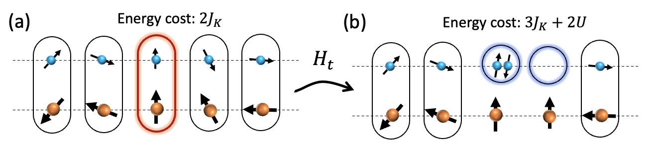
Here, and refer to the spins (magnetic moments) and and refer to conduction electrons. The spin-1/2 excitations corresponding to addition/removal of electrons and spin-1 excitations of changing local singlets into triplets. At finite electrons hop to nearby sites, creating holon-doublon virtual pairs [Fig. 2(b)]. Consequently, the vacuum contains short-lived holon-doublon pairs, which lead to short-range correlations.
III Composite Fermions: Single-Particle Properties
III.1 More details on the composite fermion operator
To characterize the single-particle excitations of the Kondo lattice, observe that acting on the ground state by the operators and each create charge-1, spin- excitations. However, instead of , we will find that the composite fermion operator
| (8) |
is the more natural operator to consider. One motivation is that transforms under the representation of . A more intuitive motivation is that the spin-electron interaction term in the Kondo lattice Hamiltonian Eq. (6) can be written as , thus is the operator which couples to electronic excitations. The factor of in Eq. (8) has been chosen so that the commutator (see Appendix A for the proof)
is unity in the strong coupling limit . The second line spoils the canonical anti-commutation of operators, however, in the strong coupling limit the expectation value of the second term is zero in the ground state, indicating that has canonical anti-commutation on average. Within the triplet sector, the expectation value of the anticommutator becomes and within the holon/doublon manifold, the expectation value of the anticommutator depends on the state of the magnetic moment. The overlap between the original and the composite electrons is
| (10) |
The right-hand side has zero average (but finite fluctuations) in the strong-coupling ground state, suggesting that and create independent excitations in average. However, and overlap due to quantum fluctuations, motivating us to compute the full Green’s function matrix involving both operators to study their associated excitations in a controlled way.
This approximately particle-like behavior of the composite-fermion has strong resemblance to the two-band model of heavy-fermions obtained in the large- mean-field theory. In such a model the spin is represented using Abrikosov fermions and the constraint is applied on average using a Lagrange multiplier. Within mean-field theory, the Kondo interaction leads to a dynamic hybridization between -electrons and -electrons [c.f. Eq. (3)]
| (11) |
The similarity of the two results suggests , implying the fact that the spin is fractionalized into spinons. In fact we can define
| (12) |
In the rest of this section we will confirm the picture outlined above by computing the full Green function using two approaches. We first use time-dependent matrix product state techniques on finite systems, then carry out a strong-coupling analysis to shed further light on the results.


III.2 Matrix Spectral Function
To examine the independence of the and fields, it is useful to combine them into a spinor
| (13) |
allowing us to define a retarded matrix Green’s function
| (14) | |||||
| (15) |
where is the step function. defines a matrix of amplitudes for the and fields. The component
| (16) |
determines the amplitude for a composite to convert to a conduction electron.
We are primarily interested in the properties of a translationally invariant Kondo lattice, with momentum-space Green’s function
| (17) | |||||
| (18) |
In our numerical calculations, we estimate this Green’s function using the expression for a translationally invariant system simply applied to finite size Green’s function . We then perform a discrete Fourier transform on to obtain
| (19) |
where is the spacing of the time-slices over the total duration of the time evolution, and the frequencies are sampled at the values .
Although we independently compute the four components of , the kinematics of the Kondo lattice imply that they are not independent, which provides us a means to test and interprete our calculations. From the Heisenberg equations of motion of the conduction electron operators in the translationally invariant limit, ,
| (20) |
where is the dispersion of the conduction electrons and is the Fourier transform of the composite fermion. It follows that
| (21) | |||||
| (22) |
When we transform these equations into the frequency domain, replacing , we see that and are entirely determined in terms of
| (23) | |||||
| (24) |
where we have suppressed the label on the propagators, and is the bare conduction electron propagator. Although these equations closely resemble the Green’s functions of a hybridized Anderson model, with hybridization , we note that represents a composite fermion.
From these results, it follows that without any approximation, the inverse matrix Green’s function can be written in the form
| (25) |
where is the one-particle irreducible composite Green’s function, determined by
| (26) |
This quantity corresponds to the unhybridized composite fermion propagator. By reinverting (25) we can express the original Green’s functions in terms of as follows
| (27) | |||||
| (28) |
These are exact results, which even hold for a ferromagnetic, , Kondo lattice. By calculating and inverting it, we can thus check the accuracy of our calculation, and we can extract the irreducible propagator .
From this discussion, we see that the matrix offers information about both the individual excitations and their hybridization. If the Kondo effect takes place, i.e if is antiferromagnetic, then we expect the formation of an enlarged Fermi surface, driven by the formation of sharp poles in the composite fermion propagator . For example, in the special case where the Green’s function develops a sharp quasiparticle pole, then we expect , allowing us to identify as an emergent hybridization.
III.3 Spectral Functions: Numerical Results
The spectral function is associated with the Green’s function by
| (29) | |||||
| (30) |
The set of values for which the spectral function has a maximum is the analogue of a band structure for an interacting system. We show the spectral functions computing using MPS for the cases of and in Fig. 3 and Fig. 4 respectively.
Figs. 3(e) and 4(e) show the quantity
| (31) |
where the denominator is entry of 2-by-2 matrix . This quantity can be interpreted as the Green’s function of the unhybridized electrons.
The most striking feature of spectral functions in Figs. 3 and 4 is the sharp and narrow bands indicative of long-lived and dispersing quasiparticles. For the larger Kondo coupling of , the spectra consist of two cosine dispersion curves shifted to positive and negative frequencies. For the smaller Kondo coupling of , the dispersion can be thought to arise as the hybridization of a dispersing band (mostly content) and a localized band (mostly content). It is apparent that in both cases, the dispersion can be approximately reproduced using a two-band fermionic model. Assuming that this is so, the quantity shown in panels 3(d) and 4(d) can be interpreted as the bare dispersion the putative fermion would need to have in order to reproduce the observed spectral functions. In both cases, a non-zero dispersion is discernible which is more significant in the case. Since in absence of Kondo interaction, composite fermions are localized , this bare dispersion is naturally associated with dynamically generated magnetic coupling between the spins due to RKKY interaction which gives rise to dispersing spinons.
III.4 Comparison with strong coupling and mean-field
It is natural to expect some of the numerical results to match those obtained in the strong Kondo coupling limit . When the decoupled sites each have the spectrum
| (32) |
where the quantum numbers and are the total spin and charge at that particular site. Creating or annihilating a particle from the ground state has the energy cost of . To understand how the ground state and single-particle excited states evolve for a finite , we have carried out a perturbative analysis for the full Green’s function in the Appendix D and found that to lowest orders in ,
| (33) |
where . The eigenenergies are
| (34) |
which confirms the picture of two hybridized bands. Here is the complex frequency and is the bare dispersion of the conduction electrons. Note that to this order, the dispersion of the bare band is not captured in agreement with previous results [31].
The quasi-particle spectrum (34) has the same form as in the large-N mean-field theory, with the difference that the value of is determined from self-consistent mean-field equation [see Appendix F]. We have plotted spectra in Fig. (5) along with predictions from strong-coupling expansion and mean-field theory. Overall, a good agreement is found albeit deviations start to appear at lower Kondo coupling of .
One artifact of the mean-field theory is that the hybridization is systematically underestimated which can be traced back to the relation between and in Eq. (3) and (11). For example, at the strong coupling limit, the mean-field theory predicts [see Appendix F]. In order to get an agreement, we had to re-scale when comparing mean-field results to numerical results on the interacting system. One can alternatively motivate this rescaling by viewing the mean-field theory as an effective model, where the parameter in the mean-field is “renormalized” from the bare hybridization.


III.5 Evolution of Single Particle States
A vivid demonstration of the particle nature of excitations can be seen by a calculating the motion of a composite fermion wavepacket. Here, it proves useful to take account of the spatially dependent normalization of the composite fermions, defining a normalized composite fermion as follows
| (35) |
where the normalization, is calculated from the measured expectation value of the anticommutator
| (36) |
Here the second expression follows from particle-hole symmetry. This normalization guarantees that the expectation value of the anti-commutator is normalized . In the ground-state, is a constant of motion, which with our definition of (8), is unity in the strong-coupling limit. However, at intermediate coupling, becomes spatially dependent near the edge of the chain.
Consider a wave-packet
| (37) |
where
| (38) |
is a normalized wave-packet centered at with momentum . The time-evolution of this one-particle-state will give rise to a state of the form
| (39) | |||||
| (40) | |||||
| (41) |
where the denotes the many-particle states that lie outside the Hilbert space of one conduction and one composite fermion. Taking the overlap with the states and , the coefficients of the wavepacket can be directly related to the Green’s functions as follows
| (42) | |||||
| (43) |
and similarly
| (44) |
where is the ground-state energy and
| (45) | |||||
| (46) |
Using the Green’s functions computed from the MPS time-evolution, we can thus evaluate the time-evolution of the wave-packet.
Figure 6 shows the evolution of the probability density of an initial Gausian wavepacket for two values of and . In the former case the composite fermion wavepacket moves ballistically until it is scattered by the boundary of the system. In the case, however, the wave-packet undergoes significant dispersion and decay with distance, appearing to ”bounce” long before reaching the wall. One possible origin of this effect, is the break-down of the Kondo effect in the vicinity of the wall, due to a longer Kondo screening length .

III.6 Interpretation of single-particle results
One of the most remarkable aspects of this comparison, is the qualitative agreement between the spectral functions derived from the matrix product, strong coupling and large expansion. In all three methods, we see that the description of the spectral function requires a two-band description. Our matrix product simulation shows that the composite fermion propagator contains sharp poles at , , which reflect a formation of composite fermion bound-states, as if the fields behave as sharp bound-states.
The single-particle excitation spectrum exhibits a coherent two-band fermionic model which continues to low . This suggests that the composite -excitations, behave as bound-states of conduction electrons and spin flips of the local moments, forming an emergent Fock space that is effectively orthogonal to that of the conduction electrons, so that and fermions are effectively independent fields. In effect, the microscopic Hilbert-space of the spin degrees of freedom has morphed into the Fock-space of the F-electrons.
In the large N limit, the composite fermion F is synonymous with a fractionalization of the local moments into half-integer spin fermions, moving under the influence of an emergent gauge field that imposes the constraints. From the single-particle excitation spectrum alone, aside from hybridization with conduction electrons, these emergent fermions appear to be free excitations: the comparison with mean-field theory suggests that the original spin is fractionalized to . As shown in A, in the strong coupling regime .
How accurate and useful is this picture? If electrons are indeed free beyond one-particle level, their higher-order Green’s functions (including two-point functions of ) would factorize into spin-1/2 fermions. We now investigate this possibility.
IV Composite Fermions: Two-Particle Properties and Spin Susceptibility
Next, we turn to the two-particle spectrum and focus on the spin susceptibility
| (47) | |||||
| (48) |
which can be probed experimentally. This function satisfies the sum-rule for any . Fig. 7 shows for two values of , computed from the Fourier transform of and using the same Fourier transform procedure as in Eq. (147). A broad incoherent region and at least one sharp dispersing mode (at low positive frequency) is visible. The latter is more pronounced at higher compared to . A spin-flip creates a localized triplet. Since only the total magnetization is conserved, the triplet can move in the lattice forming a coherent magnon band. However, in this interacting system, the magnon can decay into many-body states and the reduced weight of the coherent band is compensated by the incoherent portion of the spectrum.
In the previous section, based on the behavior of particles we conjectured that the spin is proportional to . The relationship is in fact correct in the strong Kondo coupling limit (appendix A). To test its validity beyond this limit, we compare with defined in terms of composite fermions:
| (49) | |||||
| (50) |
and involves four-point functions like . We see that the two are exactly equal, proving the relation at least within the two-particle sector.
However, while this relation seem to hold, fractionalization as seen in 1D Heisenberg AFM requires the four-point function to be expressible in terms of the convolution of two single-particle propagators. To examine this possibility, we compare the spin susceptibility with the mean-field spin susceptibility computed from the convolution of two f-electron propagators Fig. 8. The mean-field dynamical susceptibility contains a continuum of excitations bordered by two sharp lines that result from the indirect gap between the f-valence and f-conduction bands (lower sharp line) and the c-valence and c-conduction bands (upper sharp line) of the fractionalized Kondo insulator. A particularly marked aspect of the mean-field description in terms of fractionalized f-electrons is the continuum at which stretches from the hybridization gap () out to the half band-width of the conduction band. At finite this continuum evolves into a characteristic inverted triangle-shaped continuum. At strong coupling, contains a sharp magnon peak, and the triangle-shaped continuum is absent. This is clearly different from . However at weaker coupling , the MPS susceptibility is qualitatively similar to the mean-field theory, displaying the triangle-shaped continuum around and a broadened low energy feature that we can associate with the indirect band-gap excitations of the f-electrons. It thus appears that at strong-coupling, the f-electrons are confined into magnons, whereas at weak-coupling the spins have fractionalized into heavy fermions.

.

IV.1 Strong coupling and mean-field perspective
To gain further insight into the dynamical spin susceptibility, we discuss the two-particle sector from both strong coupling and mean-field perspectives. It is useful to generalize the Hamiltonian of Eq. (6) by including a Coulomb repulsion , i.e.
| (51) |
which favors one electron per site. We assume is small enough so that the ground state is smoothly connected to the original problem with .
The starting point is that at the strong coupling, all sites are singlets, and therefore the relation
| (52) |
holds. This means that can be replaced by in defined in Eq. (48), creating the following strong-coupling picture: A spin-flip can be considered as a creation of a local doublon-holon spin-triplet pair at the same site. Such a state has energies around as shown in Fig., 9. Under time-evolution, the doublon and holon can move around and recombine at site where the triplet is annihilated. Such a triplet is described by
| (53) |
Including the interaction, each holon or doublon costs an energy and . By acting on this with the Hamiltonian and projecting the result to within the two-particle excitations, we find that the wavefunction obeys the first-quantized Schrödinger equation
| (54) | |||
This is a two-particle problem, where the particles interact via the term. Note that a repulsive/attractive interaction among electrons is an attractive/repulsive interaction among doublon and holon.
In the usual regime () the interaction is attractive. While a continuum of excited states exists, the ground state is a stable magnon boundstate between doublon and holon, with a correlation length that diverges as . The continuum is essentially a fractionalized magnon into doublon and holon pairs as can be seen in the case. It is natural to expect that due to interactions not considered, the doublon-holon pair decay into the ground state. For an attractive , the interaction between doublon and holon is repulsive, rendering the bound-state highly excited and unstable.
The eigenstates can be used to compute the spin-susceptibility . The result is shown in Appendix E. The result at the strong coupling contains a magnon band in good agreement with MPS results. This indicates that while a spin-flip has fractionalized into a doublon-holon pair, there are residual attractive forces in a Kondo insulator that bind the two.
On the other hand, at the weak coupling limit, the strong-coupling analysis is incapable of reproducing MPS results around . This suggests that renormalizes to zero in the small momentum limit. As seen in Fig. 8(b) in the weak-coupling limit, the strong magnon-like resonance in the MPS dynamical spin susceptibility, broadens and merges with the triangular feature around , in sharp contrast to the strong coupling results and more closely resembling the mean-field theory [Fig. 8(d)].
To capture the doublon-holon interaction and the magnion band, the mean-field theory be improved by including a momentum-dependent residual interaction between f-electron quasi-particles within a random-phase-approximation (RPA) framework. The resulting susceptibility can be written as
| (55) |
The RPA results is shown in Fig 8(e,f) for a constant in the strong coupling case and in the weak-coupling case, both in good agreement with the MPS results.
Overall, these results indicate that the low-lying spin-1 charge-neutral excitation of the ground state can be regarded as fractionalized into spin-1/2 charge-e single particle excitations that have some residual attraction in one-dimension, forming a magnon branch in the dynamical spin-susceptibility. The disappearance of this magnon branch at in the weak-coupling regime and its comparison with RPA suggests that at long distances the residual interaction disappears, leading to deconfined quasi-particles.
V Conclusion
By contrasting strong coupling, mean-field theory and matrix product calculations of the dynamics of the one dimensional Kondo insulator, we gain an important new perspective into the nature of the excitations in this model. There are a number of key insights that arise from our results.
Firstly, we have been able to show that the composite fermion, formed between the conduction electrons and localized moments behaves as an independent fermionic excitation, giving rise to a two-band spectrum of charge , spin- excitations, with hybridization between the electrons and the independent, composite fermions. Our results are remarkably consistent with the mean-field treatment of the Kondo insulator.
By contrast, our examination of the dynamical spin susceptibility paints a more nuanced picture of the multi-particle excitations. At strong-coupling, we can explicitly see that the triplet holon and doublon combination created by a single spin-flip form a bound magnon, giving rise to a single magnon state in the measured dynamical susceptibilty. Thus at strong coupling, the spin excitation spectrum shows no sign of fractionalization. On the other hand, it can be easily checked that spin-singlet charge-2e excitations are always deconfined. Essentially, two dobulons (or two holons) can never occupy the same site, very much as same-spin electrons avoid each other due to Pauli exclusion, and thus do not interact.
However, at weaker coupling, the dynamical susceptibility calculated using MPS methods, displays a dramatic continuum of triplet excitations with an inverted triangle feature at low momentum, characteristic of the direct band-gap excitations across a hybridized band of conduction and f-electrons, and high momentum feature that resembles the indirect band-gap excitations of heavy f-electrons. These results provide clear evidence in support of a fractionalization picture of the 1D Kondo insulator at weak coupling. Based on these results, it is tempting to suggest that there are two limiting phases of the 1D Kondo insulator: a strong coupling phase in which the f-electrons are confined into magnons, and a deconfined weak-coupling phase where the local moments have fractionalized into gapped heavy fermions The emergence of a continuum in the spin-excitation spectrum at weak coupling may indicate that that the confining doublon-holon interaction at strong coupling, either vanishes, or changes sign at weak coupling, avoiding the formation of magnons.
V.1 Further Directions
It would be very interesting to extend these results to two dimensions. The strong-coupling analysis of the composite fermion Green’s function and the doublon-holon bound-states can be extended to higher dimensions, where it may be possible to calculate a critical at which confining doublon-holon bound-state develops. Further insight might be gained into the two-dimensional dimensional Kondo insulator using matrix-product states on Kondo-lattice strips, or alternatively, by using fully two dimensional tensor-network approaches or sign-free Monte-Carlo methods [13].
V.2 Discussion: Are heavy fermions in the Kondo lattice fractionalized excitations?
The 1D Kondo lattice is the simplest demonstration of Oshikawa’s theorem [42]: namely the expansion of a Fermi surface through spin-entanglement with a conduction electron sea. Traditionally, the expansion of the Fermi surface in the Kondo lattice is understood by regarding the Kondo lattice as the adiabatic continuation of a non-interacting Anderson model from small, to large interaction strength[43]. Yet viewed in their own right, the “f-electron” excitations of the Kondo lattice are emergent.
Our calculations make it eminently clear that in the half-filled 1D Kondo lattice, the f-electrons created by the fields
| (56) |
form an emergent Fock space of low energy, charge excitations that expand the Fermi sea from a metal, to an insulator. Less clear, is the way we should regard these fields from a field-theoretic perspective. From the large- expansion it is tempting to regard heavy-fermions as a fractionalization of the localized moments, . Our calculations provide support for this picture in the weak-coupling limit of the 1D Kondo lattice, where we see a intrinsic dispersion of the underlying electrons, reminiscent of a spin liquid, and a continuum of excitations in the dynamical spin susceptibility.
Yet the use of the term “fractionalization” in the context of the Kondo lattice is paradoxical, because the excitations so-formed are self-evidently charged. Field-theoretically, the spinons transform into heavy fermions, acquiring electric charge while shedding their gauge charge via an Anderson-Higgs effect that pins the internal spinon and external electromagnetic gauge fields together.
Why then, can we not regard the f-electrons of the Kondo lattice as “Higgsed”-fractionalized excitations? This is because the classical view of confinement [44] argues that confined and Higgs phases are adiabatic limits of single common phase: i.e. the excitations of a Higgs phase are confined. Yet on the other hand, we can clearly see the one and two-particle f-electron excitations, born from the localized moments, not only in the large field theory, but importantly, in the matrix product-state calculations of the 1D Kondo lattice. Moreover, a recent extension of Oshikawa’s theorem extends to all Kondo lattices [45], suggests that the large picture involving a fractionalization of spins into heavy fermions is a valid description of the large Fermi surface in the Kondo lattice. How do we reconcile these two viewpoints? Further work, bringing computational and analytic techniques together, extending our work to higher dimensions will help to clarify these unresolved questions.
Y. K. acknowledges discussions with E. Huecker. This research was supported by the U. S. National Science Foundation division of Materials Research, grant DMR-1830707 (P. C. and also, Y. K during the initial stages of the research).
Appendix A commutation relations
The composite fermion operators have the expression
| (57) |
which means
| (58) |
The same factor of appears in strong coupling expansion of multi-channel lattices [46]. The anti-commutation relations are
| (59) |
We use the identities
| (62) | |||||
| (63) |
and
| (64) |
to recast (59) as
| (65) | |||||
Using
| (66) |
we can simplify the anti-commutator to
Now, we have
| (68) |
from which we conclude
| (69) |
When inserted into (A), the terms in the parenthesis give zero (last term vanishes under antisymmetrization and the first two cancel one-another), so that
Now since and we have
| (71) |
which we can write as
In the strong-coupling limit, the first and second term inside the square brackets vanish, and in this limit the anticommutator is normalized to unity.
Appendix B Equivalence between the F-spin and local moment at strong coupling.
Appendix C Appendix: Sum-rule on wavefunction weight
| (77) |
| (78) |
Then, the total weight is
| (79) | |||
Appendix D Strong coupling expansion - Single-particle excitations
At strong coupling, the ground state is
| (80) |
where and refer to the spins (magnetic moments) and and refer to conduction electrons. To determine the energy of this state, note that
| (84) | |||||
Therefore the state has energy where is the length of the system. The action of on creates doublon-holon pairs whose corresponding spins are in a spin-singlet, i.e.
| (85) |
where
| (86) | |||
| (87) |
This excited state has energy , so the second-order correction to the strong-coupling ground state energy is
| (88) |
leading to the energy . The correction to the wavefunction is
i.e. there will be virtual doublon-holon pairs whose corresponding spins are in a singlet state . What are the single quasi-particle excitations of this ground state? We act on the ground state with
| (89) |
Note that , where for . Assuming is a good quantum number we can find
| (90) | |||
| (91) | |||
| (92) | |||
| (93) |
in terms of single doublon and holon states defined as
| (94) | |||
| (95) |
with energy
| (96) |

Using these and the spectral representation
| (97) | |||||
we find the Green’s function
where . This can be written as
| (100) |
So to lowest order in we get
| (101) |
and we can interpret as a hybridization between the conduction and composite f-electron. The real-space Green’s function can be computed from via
| (102) |
Appendix E Strong coupling expansion - Two-particle excitations
Single particle excitations are holons and doublons. The corresponding wavefunctions are
| (103) |
and these have the energies where and .
Spin-excitations belong to the two-particle excitation spectrum. A spin-triplet excitation has the wavefunction
| (104) |
Such a state has energies around . By acting on this with the Hamiltonian and projecting to stay within two-particle excitations, we find that the wavefunction obeys the first-quantized Schrödinger equation
| (105) | |||
We solve this equation using the following ansatz
| (106) | |||||
This wavefunction is labelled by quantum numbers and for doublon and holon respectively. However, note that in a typical scattering event . By plugging this wavefunction into the Schrödigner equation, we find that the doublon-holon pair state has energy
| (107) |
Furthermore, and
| (108) |
where
| (109) |
The right-hand side has to be this form, because after shift to the right . So, we find
| (110) |
But we could also go left with the holon. It folows that
| (111) |
Combining these equations we see that
| (112) |
Comparing this and the action of the translation operator on wavefunction, this is nothing but . Using these, the Schrodinger equation becomes
| (113) |
. The gives
| (114) |
We can also find the corresponding eigenvector:
| (115) |
where we have used . This can be used to find that and . We also have
| (116) |
This fixes the wavefunction up to a normalization factor which is easily determined. So, we choose . In the following, we label the doublon-holon state with center of mass and relative momenta and respectively.
| (117) |
Spin-susceptibility
We are interesting in computing the zero-temperature dynamic spin susceptibility defined by
| (118) | |||||
| (119) |
In the second line we have used that
| (120) |
By plugging-in
| (121) |
we find
where
| (122) | |||||
When taking Fourier transform
| (123) |
becomes (the positive freq. part only)
| (124) |
Appendix F Mean-field theory
Representing the spin in Eq. (1) with fermionis along with a constraint and decoupling the resulting four-fermion interaction using a Hubbard-Stratonovitch transformation, we arrive at
| (125) |
where and and the Lagrange multiplier imposes the constraint on average. At p-h symmetry, considered here, . The Hamiltonian (125) can be diaganalized using a SO(2) rotation
| (126) |
and the eigenenergies are
| (127) |
Due to -periodicity of the , we are free to choose either the period or . We choose the former interval, because the angle evolves more continuously in the Brillion zone. Therefore,
| (128) |
The relation between Kondo couling and the dynamic hybridization is given by
| (129) |
Assuming , , in the continuum limit,
| (130) |
where is the complete elliptic integral of the first kind. The strong-coupling (large ) limit of this integral is . We can use this mean-field theory to compute the retarded Green’s function
| (131) |
as well as (anti-)time-ordered Green’s functions
| (132) | |||||
with
| (133) |
These together with .
Appendix G Two-particle excitations - Random phase approximation
In the non-interacting limit, the only contribution to Eq. (119) is the disconnected part coming from Wick’s contraction
| (134) |
For non-interacting systems, we get the usual result
| (135) |
Therefore, we could assume that this is just the non-interacting but multiplied by the factor . Furthermore, the hopping of holons and doublons is exactly the same. So, we propose
| (136) |
where
| (137) |
This is shown in the figure. However, the magnon band is missing, even if we include RPA:
| (138) |
Appendix H MPS Methods for Computing Green Functions
In order to calculate Green’s function , spin susceptibility and , we first calculate the ground state by the DMRG method. The ground state is represented by site matrix product state (MPS). The spin sites of dimension 2 are located on the odd sites with the remaining conduction electrons on the even sites of dimension 4. The bond dimensions are determined automatically, and controlled by a truncation error threshold or cutoff of in the ground state calculation.
The Green’s function are defined in Eq. (15). To obtain the retarded and , we need to calculate different components of Green’s function, such as , , , etc. These terms come out because there are both and degrees of freedom, and also we need to both greater and lesser Green’s function to compute the retarded Green’s function. Without loss of generality, we take as an example. The other components are calculated by a similar approach.
| (139) | |||||
| (140) | |||||
| (141) | |||||
| (142) |
where is the ground state energy. The second equal sign holds because translational invariance of . From the third line, we choose the Heisenberg picture. It can written into the overlap of two time evolving MPS.
| (143) |
We first apply one on-site operator ( to the ground state. Two groups of MPS are obtained depending on and , then we use the time evolving block decimation (TEBD) [38, 40] to time evolve for and . In our calculation, instead of time evolving the right ket for , we evolve the bra for and ket for . Recalling that the bond dimension of an MPS generically grows exponentially under real-time evolution, splitting the time and equally distributing gates onto the bra and ket allows us to work with two MPS with significantly smaller bond dimension rather than one MPS with a large bond dimension. We obtain and , which are defined as
| (144) | |||||
| (145) |
The total time slot is split into many time slice of . For every time step, we compute the Green function by calculate the overlap between MPS.
The time evolution reaches a certain time . The resolution in frequency domains depends on . . The longer time we run, we get more find details in . In our calculation, we checked the measurement results from different and confirmed our results converged when .
The MPS bond dimension grows so the MPS bond dimension requires truncation. During the time evolving, we have tried different cut off error from to . As a result, the green function for has already converged.
Having obtained and , the retarded green function can be derived by
| (146) |
We can calculate the retarded Green’s function in the domain by Fourier transform
| (147) |
Appendix I Spin-susceptibility within mean-field theory
We can write the spin-susceptibility as
so that
| (149) |
Going to (retarded real) frequency domain
For the mean-field calculations, we use the notation in Appendix B of [47]. The within mean-field is given by
| (151) |
where , are defined in the appendix. Plugging-in Eq. (1) we find
Both term are there, but for only the first term contributes to the imaginary part
There were some numerical errors previously. Next, we plot this function assuming .

We can also do RPA on this. We define
| (154) |
Appendix J Parallelization of MPS Calculations
The Green’s function at a given time is a matrix defined in domain. The calculation of each entry involves independent time-evolution calculations and overlaps of different wave functions s and s. These wavefunctions originate with creation and annihilation operators acting on different sites . So we can parallelize these calculations and significantly reduce the time to solution. For each time slice or value of , the computation contains two parts, the time evolution and measurement.
The time evolution of s and s are independent of each other and consume approximately same amount of time, which can run in different threads with minor data exchange. In total, there are number of wave functions, which can be parallelized with no overhead cost, and scale well with increasing number of threads.
The measurement of the Green’s functions matrix involves calculating the overlap of s at different sites and . Both and run from 1 to . And the computation of these overlaps are independent, which can be computed with threads.
The time evolution step takes the dominant amount of time, because each time evolution requires application of series of gates and repeating singular value decomposition to keep bond dimension increasing, which contributes to a large prefactor before . Though the measurement scales as , the overlap operation is much faster.
References
- Menth et al. [1969] A. Menth, E. Buehler, and T. H. Geballe, Magnetic and semiconducting properties of , Phys. Rev. Lett. 22, 295 (1969).
- Mott [1974] N. F. Mott, Rare-earth compounds with mixed valencies, The Phil. Mag. 30, 403 (1974).
- Doniach [1977] S. Doniach, The kondo lattice and weak antiferromagnetism, Physica B+C 91, 231 (1977).
- Aeppli and Fisk [1992] G. Aeppli and Z. Fisk, Kondo Insulators, Commun.Condens.Matter 16, 155 (1992).
- Riseborough [2000] P. Riseborough, Heavy fermion semiconductors, Advances in Physics 49 (2000).
- Kasuya [1956] T. Kasuya, A Theory of Metallic Ferro- and Antiferromagnetism on Zener’s Model, Progress of Theoretical Physics 16, 45 (1956).
- Lacroix and Cyrot [1979] C. Lacroix and M. Cyrot, Phase diagram of the kondo lattice, Phys. Rev. B 20, 1969 (1979).
- Coleman [1984] P. Coleman, New approach to the mixed-valence problem, Phys. Rev. B 29, 3035 (1984).
- Read et al. [1984] N. Read, D. M. Newns, and S. Doniach, Stability of the kondo lattice in the large- limit, Phys. Rev. B 30, 3841 (1984).
- Auerbach and Levin [1986] A. Auerbach and K. Levin, Kondo bosons and the kondo lattice: Microscopic basis for the heavy fermi liquid, Phys. Rev. Lett. 57, 877 (1986).
- Millis and Lee [1987] A. J. Millis and P. A. Lee, Large-orbital-degeneracy expansion for the lattice anderson model, Phys. Rev. B 35, 3394 (1987).
- [12] P. Coleman, Constrained quasiparticles and conduction in heavy-fermion systems, Phys. Rev. Lett. 59, 1026.
- Danu et al. [2021] B. Danu, Z. Liu, F. F. Assaad, and M. Raczkowski, Zooming in on heavy fermions in kondo lattice models, Phys. Rev. B 104, 155128 (2021).
- [14] H. Tsunetsugu, M. Sigrist, and K. Ueda, The ground-state phase diagram of the one-dimensional Kondo lattice model, Reviews of Modern Physics 10.1103/revmodphys.69.809.
- Fye and Scalapino [1990] R. M. Fye and D. J. Scalapino, One-dimensional symmetric kondo lattice: A quantum monte carlo study, Phys. Rev. Lett. 65, 3177 (1990).
- Troyer and Würtz [1993] M. Troyer and D. Würtz, Ferromagnetism of the one-dimensional kondo-lattice model: A quantum monte carlo study, Phys. Rev. B 47, 2886 (1993).
- Raczkowski and Assaad [2019] M. Raczkowski and F. F. Assaad, Emergent coherent lattice behavior in kondo nanosystems, Phys. Rev. Lett. 122, 097203 (2019).
- Yu and White [1993] C. C. Yu and S. R. White, Numerical renormalization group study of the one-dimensional kondo insulator, Phys. Rev. Lett. 71, 3866 (1993).
- Sikkema et al. [1997] A. E. Sikkema, I. Affleck, and S. R. White, Spin gap in a doped kondo chain, Phys. Rev. Lett. 79, 929 (1997).
- McCulloch et al. [1999] I. P. McCulloch, M. Gulacsi, S. Caprara, A. Jazavaou, and A. Rosengren, Phase diagram of the 1d kondo lattice model, Journal of Low Temperature Physics 117, 323 (1999).
- Shibata and Ueda [1999] N. Shibata and K. Ueda, The one-dimensional kondo lattice model studied by the density matrix renormalization group method, Journal of Physics: Condensed Matter 11, R1 (1999).
- Peters and Kawakami [2012] R. Peters and N. Kawakami, Ferromagnetic state in the one-dimensional kondo lattice model, Phys. Rev. B 86, 165107 (2012).
- Zachar et al. [1996] O. Zachar, S. A. Kivelson, and V. J. Emery, Exact results for a 1d kondo lattice from bosonization, Phys. Rev. Lett. 77, 1342 (1996).
- Tsvelik and Yevtushenko [2019] A. M. Tsvelik and O. M. Yevtushenko, Physics of arbitrarily doped kondo lattices: From a commensurate insulator to a heavy luttinger liquid and a protected helical metal, Phys. Rev. B 100, 165110 (2019).
- Tsunetsugu et al. [1997] H. Tsunetsugu, M. Sigrist, and K. Ueda, The ground-state phase diagram of the one-dimensional kondo lattice model, Rev. Mod. Phys. 69, 809 (1997).
- Basylko et al. [2008] S. A. Basylko, P. H. Lundow, and A. Rosengren, One-dimensional kondo lattice model studied through numerical diagonalization, Phys. Rev. B 77, 073103 (2008).
- Lobos et al. [2015] A. M. Lobos, A. O. Dobry, and V. Galitski, Magnetic end states in a strongly interacting one-dimensional topological kondo insulator, Phys. Rev. X 5, 021017 (2015).
- Zhong et al. [2017] Y. Zhong, Y. Liu, and H.-G. Luo, Topological phase in 1d topological kondo insulator: Z2 topological insulator, haldane-like phase and kondo breakdown, The European Physical Journal B 90, 10.1140/epjb/e2017-80102-0 (2017).
- Zhong et al. [2018] Y. Zhong, Q. Wang, Y. Liu, H.-F. Song, K. Liu, and H.-G. Luo, Finite temperature physics of 1d topological kondo insulator: Stable haldane phase, emergent energy scale and beyond, Frontiers of Physics 14, 10.1007/s11467-018-0868-x (2018).
- Khait et al. [2018] I. Khait, P. Azaria, C. Hubig, U. Schollwöck, and A. Auerbach, Doped kondo chain, a heavy luttinger liquid, Proceedings of the National Academy of Sciences 115, 5140 (2018), https://www.pnas.org/content/115/20/5140.full.pdf .
- Trebst et al. [2006] S. Trebst, H. Monien, A. Grzesik, and M. Sigrist, Quasiparticle dynamics in the kondo lattice model at half filling, Phys. Rev. B 73, 165101 (2006).
- Smerat et al. [2009] S. Smerat, U. Schollwöck, I. P. McCulloch, and H. Schoeller, Quasiparticles in the kondo lattice model at partial fillings of the conduction band using the density matrix renormalization group, Phys. Rev. B 79, 235107 (2009).
- Appelbaum [1966] J. Appelbaum, ”” exchange model of zero-bias tunneling anomalies, Phys. Rev. Lett. 17, 91 (1966).
- Anderson [1966] P. W. Anderson, Localized magnetic states and fermi-surface anomalies in tunneling, Phys. Rev. Lett. 17, 95 (1966).
- Pustilnik and Glazman [2001] M. Pustilnik and L. I. Glazman, Kondo effect in real quantum dots, Phys. Rev. Lett. 87, 216601 (2001).
- Maltseva et al. [2009] M. Maltseva, M. Dzero, M. Dzero, P. Coleman, and P. Coleman, Electron cotunneling into a kondo lattice, Physical Review Letters 103, 206402 (2009).
- Schollwöck [2011] U. Schollwöck, The density-matrix renormalization group in the age of matrix product states, Annals of Physics 326, 96 (2011).
- Vidal [2004] G. Vidal, Efficient simulation of one-dimensional quantum many-body systems, Phys. Rev. Lett. 93, 040502 (2004).
- Daley et al. [2004] A. J. Daley, C. Kollath, U. Schollwöck, and G. Vidal, Time-dependent density-matrix renormalization-group using adaptive effective hilbert spaces, Journal of Statistical Mechanics: Theory and Experiment 2004, P04005 (2004).
- White and Feiguin [2004] S. R. White and A. E. Feiguin, Real-time evolution using the density matrix renormalization group, Phys. Rev. Lett. 93, 076401 (2004).
- Fishman et al. [2022] M. Fishman, S. R. White, and E. M. Stoudenmire, The ITensor Software Library for Tensor Network Calculations, SciPost Phys. Codebases , 4 (2022).
- Oshikawa [2000] M. Oshikawa, Topological approach to luttinger’s theorem and the fermi surface of a kondo lattice, Phys. Rev. Lett. 84, 3370 (2000).
- Martin [1982] R. M. Martin, Fermi-surface sum rule and its consequences for periodic Kondo and mixed-valence systems, Phys. Rev. Lett. 48, 362 (1982).
- Fradkin and Shenker [1979] E. Fradkin and S. H. Shenker, Phase diagrams of lattice gauge theories with higgs fields, Phys. Rev. D 19, 3682 (1979).
- Hazra and Coleman [2021] T. Hazra and P. Coleman, Luttinger sum rules and spin fractionalization in the su() kondo lattice, Phys. Rev. Res. 3, 033284 (2021).
- Ge and Komijani [2022] Y. Ge and Y. Komijani, Emergent spinon dispersion and symmetry breaking in two-channel kondo lattices, Phys. Rev. Lett. 129, 077202 (2022).
- Wugalter et al. [2020] A. Wugalter, Y. Komijani, and P. Coleman, Large- approach to the two-channel kondo lattice, Phys. Rev. B 101, 075133 (2020).