Matrix Product Density Operators: when do they have a local parent Hamiltonian?

A general open boundary (uniform) MPDO $\rho\in\mathcal{S}(\mathcal{H}_{n})$ is a quantum state $\rho$ written as

where each $\{A_{k}^{s_{i}s^{\prime}_{i}}\}_{s_{i},s^{\prime}_{i}}$ is a set of $D$-dimensional matrices and $|L\rangle,|R\rangle$ are $D$-dimensional vectors with a constant $D$. Here, $A_{k}^{s_{1}s^{\prime}_{1}},|L\rangle$ and $|R\rangle$ are chosen so that positivity $\rho\geq 0$ is satisfied for arbitrary $n$. This is a non-trivial condition and in general it is computationally hard to determine whether a given MPO is positive or not PhysRevLett.113.160503 . In this paper, we will specialize to specific sub-classes of MPDO to guarantee the positivity of the state.

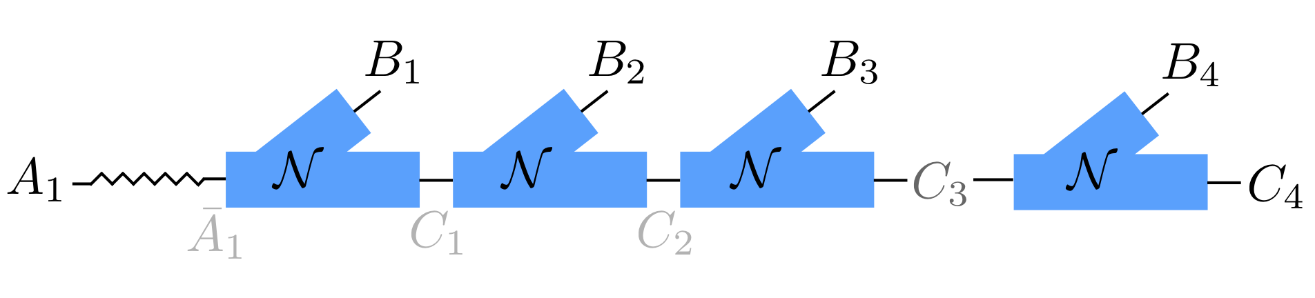
Throughout this paper, we consider MPDO constructed by concatenating Completely-Positive (CP) maps, i.e., locally purifiable MPDO. Let $\mathcal{H},\mathcal{K}$ be finite-dimensional Hilbert spaces and $\mathcal{N}:\mathcal{B}(\mathcal{H})\to\mathcal{B}(\mathcal{K}\otimes\mathcal{H})$ be a 1-input/2-output CP-map where one of the two output systems has the same dimension as the input. We interchangeably refer such a map as a Y-shaped map. For some initial state $\sigma$ and $\ell\in\mathbb{N}$, we obtain a (possibly unnormalized) state $\rho^{\sigma}_{\ell}(\mathcal{N})\in\mathcal{S}(\mathcal{K}^{\otimes\ell}\otimes\mathcal{H})$ defined by

where $\rm id_{\mathcal{K}}$ is the identity map on $\mathcal{K}$. We mostly abbreviate $\rho_{\ell}^{\sigma}(\mathcal{N})$ as $\rho_{\ell}^{\sigma}$. This kind of states are classified as a finite-dimensional $C^{*}$-finitely correlated states Fannes1992  ²²2Eq. (4) contains states without the consistency constraint imposed on the input state $\mathrm{Tr}_{B}\rho^{\sigma}_{BC}=\sigma$, which is required for $C^{*}$-infinite finitely correlated states.. By using the Kraus representation $\mathcal{N}(X)=\sum_{i}T_{i}XT_{i}^{\dagger}$, one can easily verify $\rho_{\ell}^{\sigma}$ is a MPDO.

The normalization $\mathrm{Tr}\rho^{\sigma}_{\ell}=1$ is guaranteed when $\sigma$ is a quantum state and $\mathcal{N}$ is a quantum channel, i.e., CP and Trace-Preserving (CPTP) map. Since 1D local Gibbs states always have exponentially decaying two-point correlation Araki1969 , we are interested in Eq. (4) with finite correlation length. The MPDO has a finite correlation length if $\mathrm{Tr}_{\mathcal{K}}\circ\mathcal{N}$ has unique maximum eigenvalue 1, and especially the correlation length is exactly zero when $\mathrm{Tr}_{\mathcal{K}}\circ\mathcal{N}$ is a constant channel (Fig. 3). The choice of $\sigma$ is rather arbitrary in finite systems. For convenience we mainly choose $\sigma$ as one side of the maximally entangled state, and denote the corresponding state on $\mathcal{H}\otimes\mathcal{K}^{\otimes\ell}\otimes\mathcal{H}$ by $\rho_{\ell}$. We often denote $A$ and $C$ to be two systems $\mathcal{H}$ at the end, and $B_{i}\,(i=1,...,\ell)$ to be the remaining systems $\mathcal{K}$. Note that we can recover arbitrary $\rho^{\sigma}_{\ell}$ from $\rho_{\ell}$ by applying a suitable positive operator on $A$, which is the other side of the maximally entangled state $\sigma_{A\bar{A}}$, and then trace out $A$.

When we further perform a projective measurement on $B$ to Eq. (4) in the computational basis $\{|s_{1}s_{2}...s_{l}\rangle_{B}\}$, the output subsystem ${\bar{B}}$ becomes entirely classical (Fig. 4). The corresponding Y-shaped map $\mathcal{N}$ can then be decomposed into $\mathcal{N}[\cdot]=\sum_{s_{k}}|s_{k}\rangle\langle s_{k}|\otimes\mathcal{M}_{s_{k}}[\cdot]$, where $\mathcal{M}_{s}[\cdot]$ is a CP self-map defined as

Note that if $\mathcal{N}$ is TP, then $\sum_{s}\mathcal{M}_{s}$ is a CPTP-map and thus $\{\mathcal{M}_{s}\}_{s}$ forms a quantum instrument.

We can rewrite the measured MPDO by

where each $\rho_{AC,b}$ is an output state with a particular measurement outcome $b=\{s_{1},...,s_{l}\}$

with probability

The quantum relative entropy $D(\rho\|\sigma):=\mathrm{Tr}\rho\log_{2}(\rho-\sigma)$ is a distance-like measure between two quantum states $\rho,\sigma$. One crucial feature of the relative entropy is that it obeys the data-processing inequality (DPI): for any states $\rho,\sigma$ and any CPTP-map $\mathcal{E}$, it follows that Linbald1975 ; Uhlmann:1977aa

The above DPI implies the monotonicity of the mutual information $I(A:C)_{\rho}:=D(\rho_{AC}\|\rho_{A}\otimes\rho_{C})$ and the conditional mutual information $I(A:C|B)_{\rho}$ under a local CPTP-map $\mathcal{E}_{C}:C\to C^{\prime}$, that is,

The equality holds if and only if there is a CPTP-map $\mathcal{R}_{C^{\prime}}:{C^{\prime}\to C}$ such that $\mathcal{R}\circ\mathcal{E}[\rho]=\rho$ Petz1986 ; Petz1988 .

Strong DPI constants, or the contraction coefficients are multiplicative factors in the above monotonicity inequalities. For the mutual information and CMI, they are defined as

where the values are bounded as $0\leq\eta_{AC}(\mathcal{E}_{C}),\eta_{ABC}(\mathcal{E}_{C})\leq 1$ by monotonicity. Note that $\eta_{ABC}(\mathcal{E}_{C})$ reduces to $\eta_{AC}(\mathcal{E}_{C})$ by taking $B$ to be trivial. The strong DPI constants bound how much correlations are preserved after applying the channel on subsysem $C$.

In the classical case, the strong DPI constants for different quantities are equivalent.

Remarkably, $\eta_{AC}(\mathcal{E})$ and $\eta_{ABC}(\mathcal{E})$ are independent of $A,B$ in the classical case. The crucial point is that the classical mutual information and the CMI are functions of conditional probability distribution on $C$. These functions are then written by convex combinations in classical systems, and regardless of how large auxilary classical system is involved, the Carathéodory theorem implies the auxilary system can always be reduced to dimension $|C|+1$ Danninger-Uchida2001 .

Unfortunately, no analog of conditional distribution nor the Carathéodory-like cardinality bound has been found for quantum systems (see e.g., Ref. 6555753 for a discussion on this problem). Therefore the classical approach failed to work in quantum regime. For this reason, for quantum systems it remains open whether Theorem II.1 also holds, or whether the strong DPI constants are independent of the size of the auxiliary systems or not.

The CMI and Gibbs states are intimately connected. In classical systems, the Hammersley-Clifford theorem HCthm states that a (positive) probability distribution $p_{XYZ}$ is a Gibbs distribution

where $Z$ is the normalization constant, if and only if $I(X:Z|Y)_{p}=0$. Moreover, CMI can be written as

and thus the small value of the CMI implies the state is close to a Gibbs state (16). These results are naturally extended to 1D classical spin chains.

Although Eq. (17) does not hold in general quantum systems, Ref. KB16 shows the following bound:

If $\varepsilon=0$, we recover the quantum Hammersley-Clifford theorem Hayden2004 ; brown2012quantum and the Hamiltonian $H$ is the sum of terms like $-\log\rho_{A_{i},A_{i+1}}$.

When MPDO has exponentially decaying CMI for appropriate tripartitions, then we first coarse-grain sufficiently many (possibly logarithmic w.r.t. $1/\varepsilon$) neighbouring sites as one site and then apply Theorem II.2 to show that the MPDO is well-approximated by a local Gibbs state.

Note that relative entropy estimate converts to fidelity by

To characterize what information is left undisturbed by a channel, we use the theory of operator-algebra quantum-error correction Beny2007 ; Beny2007a . For a given channel $\mathcal{E}:A\to A^{\prime}$, we define the correctable algebra $\mathcal{A}(\mathcal{E})\subset\mathcal{B}(\mathcal{H}_{A})$ as

$\mathcal{A}(\mathcal{E})$ is a finite-dimensional $C^{*}$-algebra containing all observables whose information is perfectly preserved under $\mathcal{E}$. One can always perfectly recover the information associated to an observable in the correctable algebra: there exists a CPTP-map $\mathcal{R}:A^{\prime}\to A$ called recovery map such that

This implies that for any $O_{A}\in\mathcal{A}(\mathcal{E})$, there always is a corresponding observable $\mathcal{R}^{\dagger}(O_{A})$ on $A^{\prime}$ such that $\mathrm{Tr}(O_{A}\rho_{A})=\mathrm{Tr}\left(\mathcal{R}^{\dagger}(O_{A})\mathcal{E}(\rho_{A})\right)$ for all $\rho_{A}$. The condition in Eq. (22) is a generalization of the well-known Knill-Laflamme condition PhysRevLett.84.2525 in the standard quantum error correction theory, in which $\mathcal{A}(\mathcal{E})=\mathcal{B}(\mathcal{H}_{code})$ for a protected code subspace $\mathcal{H}_{code}$.

A common candidate for the recovery channel is the Petz map:

As it only features moderately in this paper, we save the vast literature on universal recovery channel elsewhere (see e.g., Junge_2018 ), and include the relevant ideas on invariant subspaces in Appendix A. This yields another characterization of the correctable algebra handy for our purposes.

Our first main result is showing that any state constructed from a bistochastic ³³3Usually, bistochastic refers to a self-map channel in the literature. Here we have higher output dimension than input, but we abuse the terminology in this paper. Y-shaped channel (CPTP-map) is exponentially close to a product state on $AB$ and $C$. This provides an upper bound of the CMI (and also the trace norm CMI in Sec. III.1.1). See Sec. IV.1 for the proof.

In this paper, we pay less attention to the case of periodic MPDO where output $C$ of channel got fed into the input $A$, as this gluing step might be tricky. In the bistochastic case this is tractable (Appendix B) and the state becomes even simpler as the maximally mixed state plus an exponentially decaying global operator. There, the parent Hamiltonian would be trivial in the thermodynamic limit.

A crucial property of bistochastic Y-shaped channels is they act as a contraction onto certain operator subspace. This implies Eq. (27) at large $\ell$, and then the CMI bound follows from the continuity of the entropy. An example of bistochastic Y-shaped channel is given as follows.

While being bistochastic is crucial to provide a decay rate defined by relative entropy in Theorem III.1, we can work with slightly general channels with a likely suboptimal decay rate. See Sec. IV.2 for the proof.

The decay of CMI for more general tripartition follows from the same argument as the bistochastic case (Theorem III.1 ). The distinction, though, is that our bound for the contraction ratio suffers from extra factor of dimension $d_{C}$ due to conversion to the completely bounded norm (Lemma V.3), so the bound is meaningful only for the noisy regime $\eta_{1,C}<(16d_{c})^{-1}$.

Although we have shown the upper bound of CMI for bistochastic Y-shaped channels, they are only a small portion of the space of channels. Here, we show another suggestive result towards Question I.1.

Remarkably, each application of $\mathcal{N}$ contracts the CMI by $\eta$, from simple application of convexity of relatively entropy and monotonicity of CMI (proof in Sec. V.2.3). Intuitively the contraction ratio is $\eta$ because the forgetful channel necessarily removes any correlation with system $AB$. The step wise decay implies the decay of CMI for any tripartition with a long conditioned system $B$, i.e. the Y-shaped channel is applied many times.

Note that any strictly positive Y-shaped channel $\mathcal{N}(\rho)>0$ always has a decomposition (54) with $F$ being the completely depolarizing channel. Moreover, for any Y-shaped channel $\mathcal{N}^{\prime}$ and any $0\leq\eta<1$, we can always construct a perturbed channel $\mathcal{N}$ in Eq. (54) satisfying $\|\mathcal{N}-\mathcal{N}^{\prime}\|_{cb}\leq 2(1-\eta)$.

In the sense that any channel can be perturbed to have a forgetful component, Proposition III.2 is true for most of quantum channels. We should note that the appropriate choice of ‘generic’ MPDO certainly depends on the constraint of the problem at hand, for example if we restrict the number of Kraus operators to be small, then strict positivity would not hold generically.

A channel with forgetful component necessarily has trivial correctable algebra, but not vice versa. We can see this fact through an explicit example.

Example: The classical channel given by the following Kraus operators has trivial correctable algebra, but has no forgetful component. Input states $|1\rangle\langle 1|,|2\rangle\langle 2|,|3\rangle\langle 3|$ are mapped to $\frac{|2\rangle\langle 2|+|3\rangle\langle 3|}{2},\frac{|1\rangle\langle 1|+|3\rangle\langle 3|}{2},\frac{|1\rangle\langle 1|+|2\rangle\langle 2|}{2}$, whose intersection is empty and thus cannot have a shared forgetful component.

We have shown the channels we considered in Sec. III.1, III.2 incur the exponential decay of CMI. For channels with a forgetful component (Proposition III.2), the exponential decay simply comes from a contraction occurring at each application of channel, and it is tempting to ask whether this is the general case. This motivates the following discussion on the data processing inequality.

First, we show that a single application of any channel with trivial correctable algebra always induces strict decay of CMI.

The proof is given in Sec. V.2.1. By regarding $\mathcal{E}$ as Y-shaped channel $\mathcal{N}_{C_{i-1}\to B_{i}C_{i}}$, we see that $I(A:C|B)_{\rho_{k}}<I(A:C|B)_{\rho_{k-1}}$ holds for each $k$ (we abuse notation $BC$ for two different lengths). Note that having trivial correctable algebra provides only a sufficient condition to have a strict decay of the CMI. There is a Y-shaped channel with non-trivial correctable algebra which obeys Eq. (69) (see Ref. KB20 for a complementary result).

Unfortunately, recursively applying Eq. (69) may not imply the exponential decay of CMI of $\rho_{\ell}$ as the decay might get slower as system $B$ gets larger. We therefore propose the following conjecture to explicitly include a contraction ratio as a strong DPI constant.

Invoking standard monotonicity inequalities(Sec. V.2.2), the contraction accumulates and thus Conjecture III.1 implies the desired exponential decay of CMI:

Conjecture III.1 holds for the channels with a forgetful component (Proposition III.2), where $\eta_{ABC}(\mathcal{E})$ does not approach 1 as $AB$ grows. In the classical case generally an unbounded auxiliary system can be reduced to have bounded dimension only depending on $C$, and for the strong DPI constants the auxiliary system can be ignored $\eta_{ABC}=\eta_{AC}=\eta_{C}$ (Theorem II.1). In the quantum case we do not know whether $AB$ can be reduced to a bounded dimension. Hence, the conjecture is open in general quantum systems and even showing its simpler variant for the mutual information (setting $B$ trivial) would be a breakthrough. Very recently the case when $A$ is classical and $B$ is trivial was proven with a contraction ratio analogous to the classical case hirche2020contraction .

A similar DPI can be proposed for the trace norm CMI.

We do not know if extra constants or factor of dimension $d_{C}$ should be present between $\eta_{1,C}$ and $\eta$ like the crude bound in Theorem III.2. The trace norm seems more tractable than mutual information in the bipartite case.

Here the contraction ratio is controlled by a bounded factor, where the dimension factor comes from bounding the completely bounded superoperator $1-1$ norm (Lemma V.3).

In this section we consider the CMI of MPDO after performing the local measurement on the computational basis of $B$. Here we do not require the original map $\mathcal{N}$ in Eq. (4) to be trace-preserving.

Condition 2 (strict positivity of all $\mathcal{M}_{s}$) is unlikely a necessary condition for the decay of CMI, but it is convenient to state. We include coarse-graining in the statement as it is sometimes needed to ensure strict positivity of all $\mathcal{M}_{s}$. For example, if the original Y-shaped CP map comes from tracing out a system much smaller than the bond dimension, then it may not be strictly positive.

A similar bound for the coarse-graining length $\xi$ for iteration of a single channel was given by the quantum Wielant inequality 5550282 : for every primitive channel $\mathcal{N}$ (with Kraus rank $p$ and Hilbert space dimension $D$), $\xi={D^{2}(D^{2}-p+1)}$ iteration guarantees full-rank output. Our Condition 1 is a multi-channel generalization: it is a sufficient condition for all possible sequences of $\mathcal{M}_{s_{\ell}}\circ\cdots\circ\mathcal{M}_{s_{2}}\circ\mathcal{M}_{s_{1}}$ generated by CP maps $\{\mathcal{M}_{1},\mathcal{M}_{2},\cdots\mathcal{M}_{n}\}$ to become strictly positive for coarse graining length $l\geq\xi:=D^{2}-p+1$. See Sec. IV.3 for the proof.

Although strict positivity (Condition 2) is NP-hard to check in general gaubert2014checking , we prove that Condition 1 can be verified in a polynomial time (see Sec. V.4.5 for the details).

We numerically verify Condition 1 (generating full algebra) for Y-shaped channels generated by Haar-random Stinespting unitary (Fig. 3, bottom). The unitaries are the same random sample $U(D^{2})$, and we have checked for computationally tractable local Hilbert space dimensions $D\leq 8.$ ⁴⁴4githubcode is the repository of the jupyter code. The code checks condition 1 for arbitary MPDO given the Kraus operators.. Both conditions imply Eq. (76), which further implies our original goal, Eq. (77).

The bistochastic assumption greatly simplifies the structure of state. The state can be decomposed into a uncorrelated state $\rho_{AB}\otimes\tau_{C}$ plus a deviation $G_{ABC}$ that is traceless on system $C$. At each application of channel in the generation of $\rho_{\ell}$, there are two key implications of being bistochastic: 1) the uncorrelated state $\rho_{AB}\otimes\tau_{C}$ is mapped to an uncorrelated state where system $C$ remains the maximally mixed state $\tau_{C}$, 2) the deviation $G_{ABC}$ contracts w.r.t the normalized Hilbert-Schimdt norm. The rest of the proofs are obtained by standard conversion between norms. The proofs of the lemmas are shown independently in Sec. V.1.

References

- (1) I. Affleck, T. Kennedy, E. H. Lieb, and H. Tasaki. Rigorous results on valence-bond ground states in antiferromagnets. Phys. Rev. Lett., 59(7), 1987.
- (2) D. Perez-Garcia, F. Verstraete, M. M. Wolf, and J. I. Cirac. Matrix product state representations. Quantum Inf. Comput., 7(5-6), 2007.
- (3) M. B. Hastings. An area law for one-dimensional quantum systems. J. Stat. Mech.-Theory. E., 2007(08), 2007.
- (4) M. Fannes, B. Nachtergaele, and R. F. Werner. Finitely correlated states on quantum spin chains. Commun. Math. Phys., 144(3), 1992.
- (5) N. Schuch, D. Perez-Garcia, and J. I. Cirac. Classifying quantum phases using matrix product states and projected entangled pair states. Phys. Rev. B, 84(16), 2011.
- (6) F. Verstraete and J. I. Cirac. Renormalization algorithms for quantum-many body systems in two and higher dimensions, arXiv:cond-mat/0407066, 2004.
- (7) A. Molnar, Y. Ge, N. Schuch, and J. I. Cirac. A generalization of the injectivity condition for projected entangled pair states. J. Math. Phys., 59(2), 2018.
- (8) M. B. Hastings. Solving gapped Hamiltonians locally. Phys. Rev. B, 73(8), 2006.
- (9) F. Verstraete, J. J. García-Ripoll, and J. I. Cirac. Matrix product density operators: Simulation of finite-temperature and dissipative systems. Phys. Rev. Lett., 93(20), 2004.
- (10) J. I. Cirac, D. Pérez-García, N. Schuch, and F. Verstraete. Matrix product density operators: Renormalization fixed points and boundary theories. Ann. Phys., 378, 2017.
- (11) K. Kato and F. G. S. L. Brandão. Quantum approximate markov chains are thermal. Commun. Math. Phys., 370(1):117–149, 2019.
- (12) M. Kliesch, D. Gross, and J. Eisert. Matrix-product operators and states: Np-hardness and undecidability. Phys. Rev. Lett., 113:160503, 2014.
- (13) H. Araki. Gibbs states of a one dimensional quantum lattice. Commun. Math. Phys., 14(2), 1969.
- (14) G. Lindblad. Completely positive maps and entropy inequalities. Commun. Math. Phys., 40(2):147–151, 1975.
- (15) A. Uhlmann. Relative entropy and the wigner-yanase-dyson-lieb concavity in an interpolation theory. Commun. Math. Phys., 54(1):21–32, 1977.
- (16) D. Petz. Sufficient subalgebras and the relative entropy of states of a von Neumann algebra. Commun. Math. Phys., 105(1):123–131, 1986.
- (17) D. Petz. Sufficiency of channels over Von Neumann algebras. Q. J. Math., 39(1), 1988.
- (18) V. Anantharam, A. Gohari, S. Kamath, and C. Nair. On hypercontractivity and a data processing inequality. 2014 IEEE International Symposium on Information Theory, 3022-3026, 2014.
- (19) G. E. D.-Uchida. Carathéodory theorem. Springer US, Boston, MA, 2001.
- (20) S. Beigi and A. Gohari. On dimension bounds for quantum systems. In 2013 Iran Workshop on Communication and Information Theory, 1–6, 2013.
- (21) J.M. Hammersley and P.E. Clifford. Markov field on finite graphs and lattices. http://www.statslab.cam.ac.uk/ grg/books/hammfest/hamm-cliff.pdf, 1971.
- (22) P. Hayden, R. Jozsa, D. Petz, and A. Winter. Structure of States Which Satisfy Strong Subadditivity of Quantum Entropy with Equality. Commun. Math. Phys., 246(2), 2004.
- (23) W. Brown and D. Poulin. Quantum Markov Networks and Commuting Hamiltonians. arXiv:1206.0755 2012.
- (24) C. Bény, A. Kempf, and D. W. Kribs. Generalization of quantum error correction via the Heisenberg picture. Phys. Rev. Lett., 98(10), 2007.
- (25) C. Bény, A. Kempf, and D. W. Kribs. Quantum error correction of observables. Phys. Rev. A, 76(4), 2007.
- (26) E. Knill, R. Laflamme, and L. Viola. Theory of quantum error correction for general noise. Phys. Rev. Lett., 84:2525–2528, 2000.
- (27) M. Junge, R. Renner, D. Sutter, M. M. Wilde, and A. Winter. Universal recovery maps and approximate sufficiency of quantum relative entropy. Ann. Henri. Poincaré., 19(10):2955–2978, Aug 2018.
- (28) D. Petz. sufficiency of channels over von neumann algebras. The Quarterly Journal of Mathematics, 39(1):97–108, 03 1988.
- (29) M. M. Wilde. From classical to quantum shannon theory, 2011.
- (30) K. Kato and F. G. S. L. Brandão. Toy model of boundary states with spurious topological entanglement entropy. Phys. Rev. Research, 2:032005, Jul 2020.
- (31) M. Sanz, D. Pérez-García, M. M. Wolf, and J. I. Cirac. A quantum version of wielandt’s inequality. IEEE Transactions on Information Theory, 56(9):4668–4673, 2010.
- (32) S. Gaubert and Z. Qu. Checking the strict positivity of Kraus maps is np-hard. arXiv:1402.1429, 2014.
- (33) A. Winter. Tight uniform continuity bounds for quantum entropies: conditional entropy, relative entropy distance and energy constraints, Commun. Math. Phys. 347(1):291-313, 2016.
- (34) M. Takesaki. Theory of operator algebras. I, volume 124 of Encyclopaedia of Mathematical Sciences. Springer-Verlag, Berlin, 2002.
- (35) C.-F. Chen, G. Penington, and G. Salton. Entanglement wedge reconstruction using the petz map. JHEP, 2020(1), Jan 2020.
- (36) V. Paulsen. Completely Bounded Maps and Operator Algebras. Cambridge Studies in Advanced Mathematics. Cambridge University Press, 2003.
- (37) M. James. Quantum markov chain mixing and dissipative engineering. PhD thesis, 2015.
- (38) D. Reeb, M. J. Kastoryano, and M. M. Wolf. Hilbert’s projective metric in quantum information theory. J. Math. Phys., 52(8):082201, 2011.
- (39) E. Kohlberg and J. W. Pratt. The Contraction Mapping Approach to the Perron-Frobenius Theory: Why Hilbert’s Metric? Math. Oper. Res., 7(2):198–210, 1982.
- (40) V. Lomonosov and P. Rosenthal. The simplest proof of Burnside’s theorem on matrix algebras. Linear Algebra Appl., 383:45 – 47, 2004. Special Issue in honor of Heydar Radjavi.
- (41) D. Pérez-García, M. M. Wolf, D. Petz, and M. B. Ruskai. Contractivity of positive and trace-preserving maps under norms. J. Math. Phys., 47(8):083506, 2006.
- (42) V. Y. Protasov and A.S. Voynov. Sets of nonnegative matrices without positive products. Linear. Algebra. Appl., 437(3):749 – 765, 2012.
- (43) M. Koashi and N. Imoto. Operations that do not disturb partially known quantum states. Phys. Rev. A, 66:022318, Aug 2002.
- (44) G. Lindblad. A general no-cloning theorem. Lett. Math. Phys., 47(2):189–196, 1999.
- (45) C. Hirche, C. Rouzé, and D. S. França On contraction coefficients, partial orders and approximation of capacities for quantum channels. arxiv:2011.05949, 2020
- (46) https://github.com/Shawnger/supplementary_MPDO
Appendix A Equivalence between correctable algebra and the Petz recovered map for bistochastic channels
The structure of CPTP self-map, the invariant subspace, and the fixed-point algebra of the dual has been studied.
Theorem A.1 (Combination of Hayden2004 ; PhysRevA.66.022318 ; lindbald1999 ).
For every CPTP self-map , the following holds:
-
1.
The invariant subspace of forms a subalgebra , with factors .
(199) -
2.
The invariant subspace of of has form
(200) with determined by , and are free.
3.
The channel restricted on the block diagonal entries has form (its acting on off-diagonal part is not as simple)
(201) and has unique fixed point
Though, when a channel has different input-output dimension, we alternatively consider the correctable algebra . It turned out to correspond to the invariant subspace of , the original channel composed with the Petz recovery map with the maximally mixed state as the reference.
Proposition A.1 (Recap of Proposition II.1).
The correctable algebra of a channel equals to the fixed-point algebra of the Petz-recovery channel composed with channel (and the dual , due to being self-adjoint).