capbtabboxtable[][\FBwidth]
Shailesh Nirgudkar, University of Lowell, Lowell, MA, USA 01854
MassMIND: Massachusetts Maritime INfrared Dataset
Abstract
Recent advances in deep learning technology have triggered radical progress in the autonomy of ground vehicles. Marine coastal Autonomous Surface Vehicles (ASVs) that are regularly used for surveillance, monitoring and other routine tasks can benefit from this autonomy. Long haul deep sea transportation activities are additional opportunities. These two use cases present very different terrains - the first being coastal waters- with many obstacles, structures and human presence while the latter is mostly devoid of such obstacles. Variations in environmental conditions are common to both terrains. Robust labeled datasets mapping such terrains are crucial in improving the situational awareness that can drive autonomy. However, there are only limited such maritime datasets available and these primarily consist of optical images. Although, Long Wave Infrared (LWIR) is a strong complement to the optical spectrum that helps in extreme light conditions, a labeled public dataset with LWIR images does not currently exist. In this paper, we fill this gap by presenting a labeled dataset of over 2,900 LWIR segmented images captured in coastal maritime environment under diverse conditions. The images are labeled using instance segmentation and classified in seven categories - sky, water, obstacle, living obstacle, bridge, self and background. We also evaluate this dataset across three deep learning architectures (UNet, PSPNet, DeepLabv3) and provide detailed analysis of its efficacy. While the dataset focuses on the coastal terrain it can equally help deep sea use cases. Such terrain would have less traffic, and the classifier trained on cluttered environment would be able to handle sparse scenes effectively. We share this dataset with the research community with the hope that it spurs new scene understanding capabilities in the maritime environment.
keywords:
Autonomous surface vehicles, long wave infrared, instance segmentation, object detection, dataset1 INTRODUCTION
In recent years, advances in deep learning algorithms have led to an exponential growth in the research on autonomy of land vehicles. Some of the key catalysts for this growth have been publicly available labeled datasets, open-source software, publication of novel deep learning architectures and increase in hardware compute capabilities. The maritime environment, with an abundance of periodic tasks such as monitoring, surveillance, and long haul transportation presents a strong potential for autonomous navigation. Availability of good datasets is a key dependency for gaining autonomy. Various types of sensors such as electro-optical (EO) cameras, LWIR cameras, radar and lidar help in collecting huge volume of data about surroundings. The challenge lies in interpreting this data and creating labeled datasets that can help train deep learning architectures.
EO cameras are predominantly used to capture images because of their versatility and the abundant Convolutional Neural Network (CNN) architectures Krizhevsky et al. (2012) that learn from labeled images. Two methods are commonly used for annotating an image. First, detecting objects of interest by drawing bounding boxes around them. Second, semantically segmenting an image in which each pixel is assigned a class label. The first method is faster as it focuses on specific targets, however, the second is more refined as it segments the entire scene.
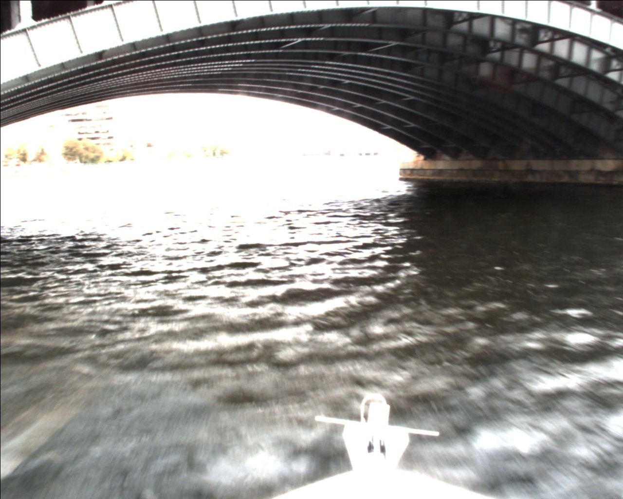
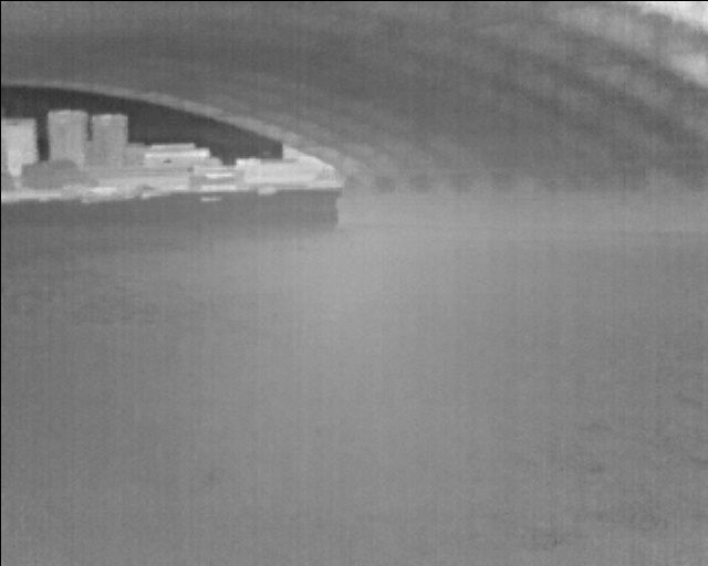
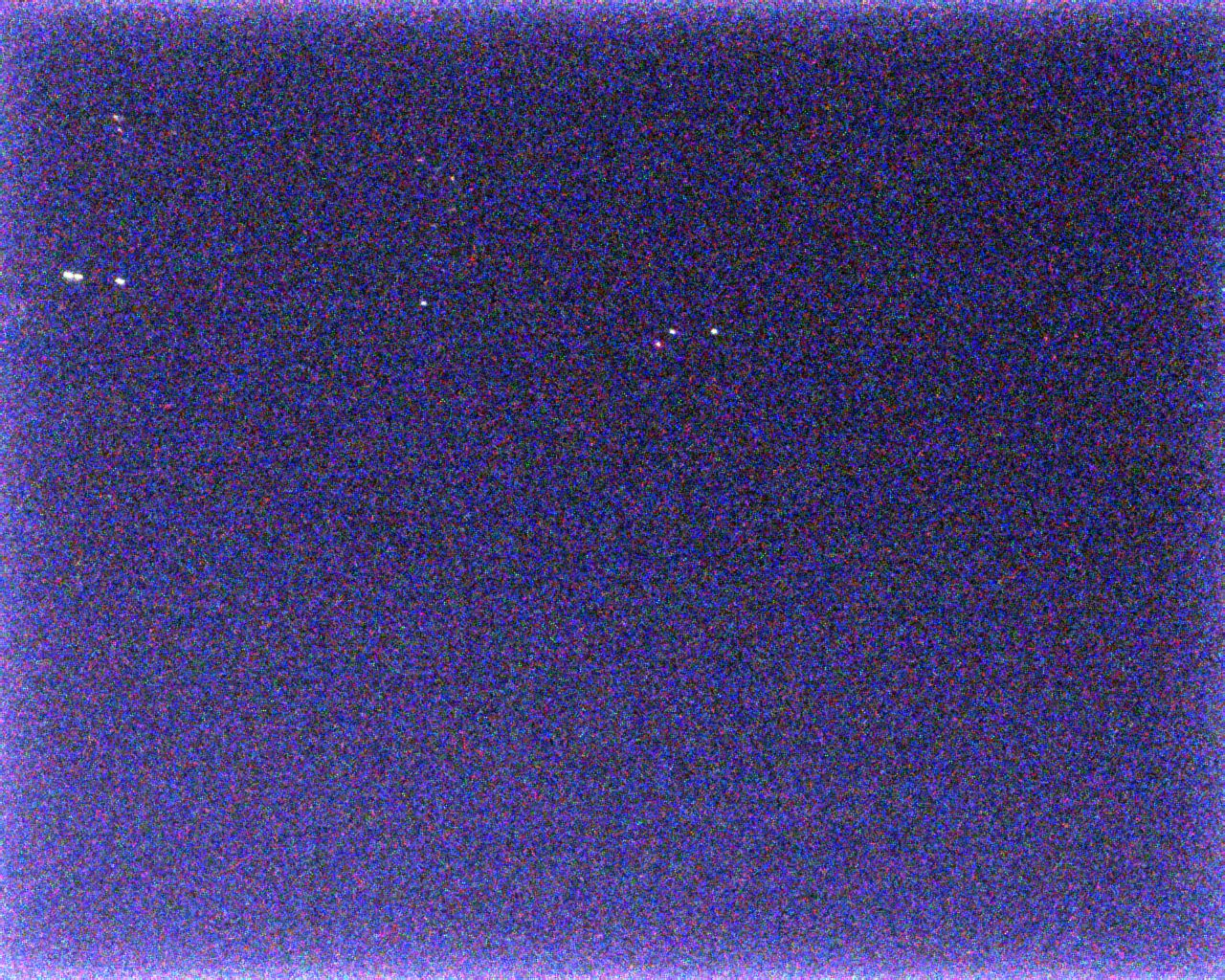
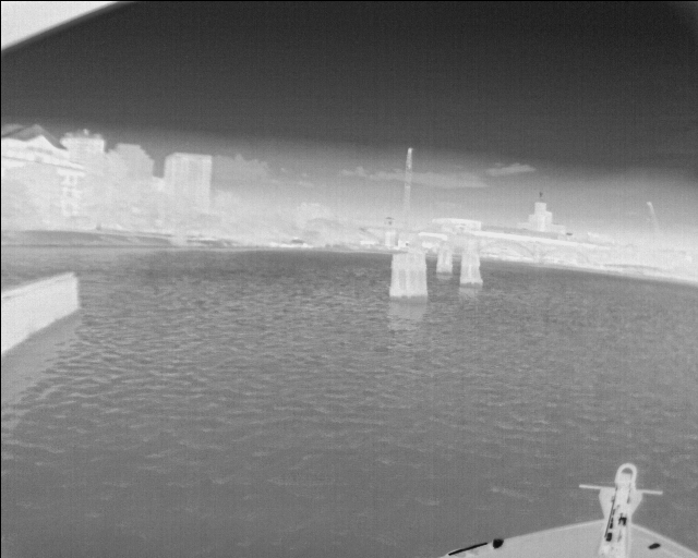
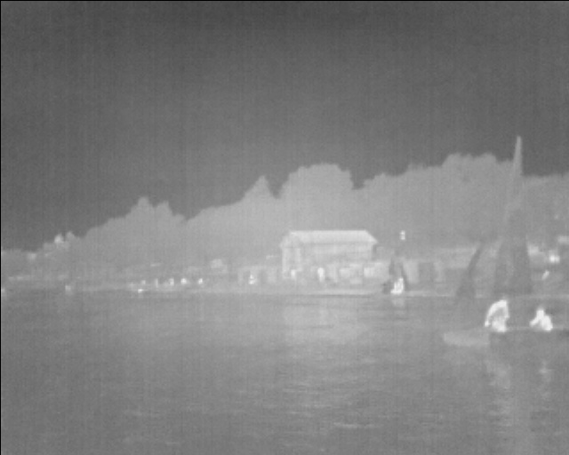
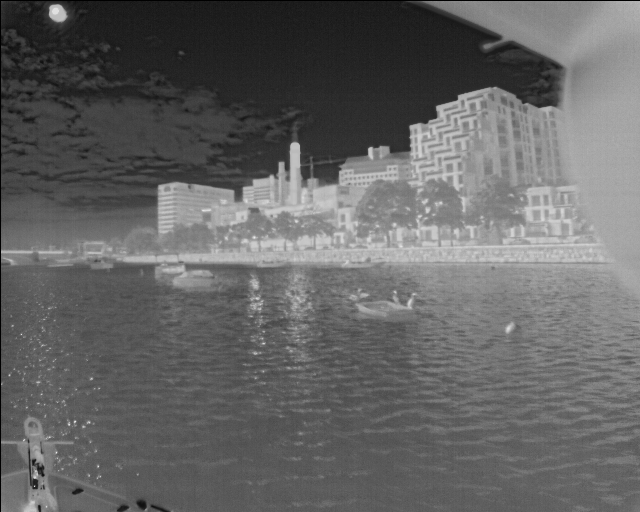
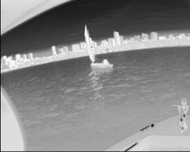
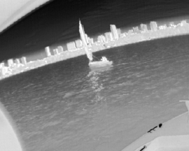
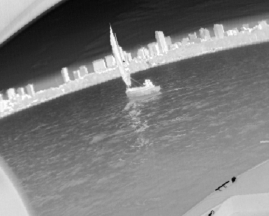
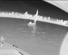
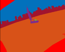
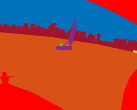
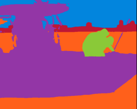
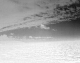
The maritime environment is predominantly exposed to sky and water and the lighting conditions are therefore quite different as compared to a ground terrain. Glitter, reflection, water dynamism and fog are common. These conditions deteriorate the quality of optical images. Horizon detection is also a common problem faced while using optical images. On the other hand, LWIR images offer distinct advantages in such extreme light conditions as shown experimentally by Robinette et al. (2019), Nirgudkar and Robinette (2021) and as shown in Fig. 1. Marine robotics researchers have used LWIR sensors in their work (Schöller et al. (2019), Rodin and Johansen (2018), Qi et al. (2011), Wang et al. (2017)). Most notably Zhang et al. (2015) has built a labeled dataset of paired visible and LWIR images of different types of ships in the maritime environment. However, there are certain limitations of this dataset which are discussed in the next section.
In this paper, we present a dataset of over 2,900 LWIR maritime images that capture diverse scenes such as cluttered marine environment, construction, living entities and near shore views across various seasons and times of the day in the Massachusetts Bay area including Charles River and Boston Harbor. The dataset images are segmented using instance and semantic segmentation into 7 classes. We also evaluate the performance of this dataset across 3 popular deep learning architectures (UNet, PSPNet, DeepLabv3) and present our findings with respect to obstacle detection and scene understanding. The dataset is publicly available and can be downloaded from the URL Nirgudkar et al. (2022). We aim to stimulate research interest in the field of perception in maritime autonomy through these dataset.
The remainder of the paper has been organized as follows. Section 2 outlines the current state of art in the maritime domain. Section 3 describes the hardware assembly that is used for data acquisition. Specifics about the dataset and segmentation methods have been elaborated in Section 4 and Section 5 presents evaluation results against the 3 architectures. We draw conclusions in Section 6 and highlight the future plan of work.
2 RELATED WORK
Significant research has gone in the field of marine robotics over the past few years and researchers have developed multiple datasets that can aid autonomy. These datasets vary in size and complexity, however, their main purpose revolves around environment monitoring and surveillance. Castellini et al. (2020) used autonomous aquatic drones and captured multivariate time series data for the purpose of water quality management. The dataset contains parameters such as water conductivity, temperature, oxygen level and is useful for time series analysis. Bloisi et al. (2015) used ASV in Venice, Italy and created a dataset of optical images for the purpose of boat identification and classification. The ground truth in this dataset is provided in the form of bounding boxes. Ribeiro (2015) captured images from an unmanned aerial vehicle (UAV) 150-300 meter above ocean surface for research on sea monitoring and surveillance. Though multi-spectrum cameras including IR cameras are used, the dataset is not annotated and hence it cannot be used readily for model training. Another problem is that the images were aerial pictures and therefore do not have the same perception properties as that of the view from a vehicle on the water surface. Zhang et al. (2015) has created a dataset of paired visible and LWIR images of various ships in the maritime environment. The annotations are provided in the form of bounding boxes around ships. However, selection is focused on those images where ships occupy more than 200 pixels of the image area. The dataset is therefore not adaptable for general use where obstacles can be in any shape or form such as buoys, small platforms, construction in water. More importantly, the images are captured from a static rig mounted on the shore and therefore lack the dynamism found in real life scenarios.
Prasad et al. (2017) has created a dataset using optical and near infrared (NIR) cameras to capture maritime scenes from a stationary on-shore location. This dataset also has some video sequences recorded from a ship but they are from a higher vantage point and hence do not clearly depict the same view as that from an ASV. Additionally, not all images in the dataset are annotated. Only a few are annotated using bounding boxes. Patino et al. (2016) has used multi-spectrum cameras to capture video segments of enacted piracy scenes. The emphasis is on threat detection and so the video sequence contains medium to large boats appearing in the frames. Since the visuals are enforced, the dataset lacks natural marine scenes that are critical for training a model. Steccanella et al. (2020) used pixel wise segmentation to differentiate between water and non-water class. The dataset contains around 515 optical images with the 2 classes. In recent years, two excellent datasets MaSTR1325 and MODS have been created by Bovcon et al. (2019) and Bovcon et al. (2021). The optical images in these datasets are semantically segmented in 3 classes and are suitable for unmanned surface vehicles (USV) navigation. However, as pointed out by Bovcon et al. (2021), bright sunlight, foam, glitter and reflection in the water deteriorate the inference quality. Small object detection poses a challenge even for the model developed by Bovcon and Kristan (2020) that is specifically designed for the maritime environment.
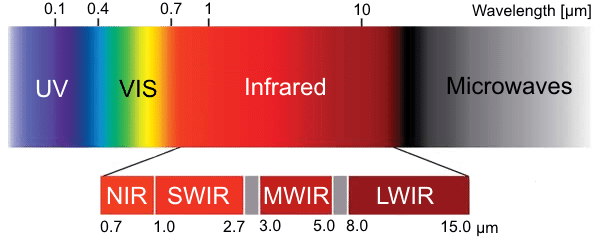
Most of these datasets are captured using EO cameras. The ones that used NIR, do not provide the benefit of LWIR as they are still dependent on visible light. As indicated in Fig. 2 EO (2022) NIR light occupies a wavelength between 0.75 to 1.4 microns and although it is a part of the Infrared spectrum, it is not caused by thermal radiation. Instead it is almost similar to visible light except that it cannot be observed by human eye. Heat or thermal radiation is the primary source of radiation for LWIR NASA (2003), Hyll (2016) and therefore LWIR is truly independent of visible light.
In a nutshell, the existing NIR/LWIR datasets lack complete scene parsing capabilities, or have been created in a controlled environment or are not publicly available. MassMIND bridges this gap and is the largest labeled dataset of its kind containing real-life LWIR images. The images have been recorded in a busy marine area as well as in not so busy ocean waters during various seasons and times of the day over a period of 2 years. The dataset has been annotated into 7 classes using instance segmentation that can be used for scene parsing during autonomous navigation.
3 SYSTEM SETUP
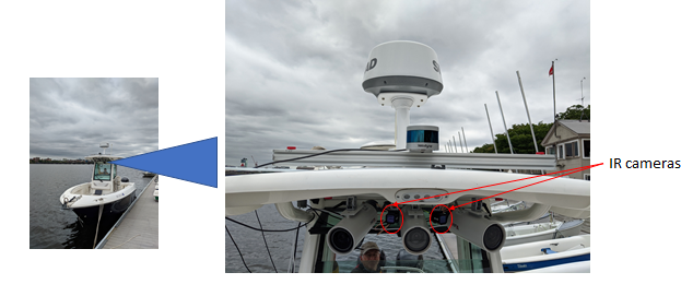
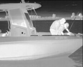
R/V Philos, an ASV owned by the Brunswick Corporation and operated by MIT Autonomous Underwater Vehicle (AUV) AUVLab (1989) lab was instrumental in collecting images for the MassMIND dataset. The ASV is equipped with 3 EO cameras, 2 Forward looking Infrared (FLIR)-LWIR cameras, a radar, a lidar, GPS and Inertial Measurement Unit (IMU). The FLIR cameras used in 2019 were entry level providing resolution of 320240 (widthheight) and horizontal field of view of 34°. These cameras were upgraded in 2020 which provided resolution of 640512 (widthheight) and horizontal field of view of 75°. Images from these sensors have slight offset with one another due to the placement of EO and FLIR cameras as shown in Fig. 3. Table 1 shows technical specifications of the FLIR ADK cameras used in the setup in 2019 and later. Additional details of the ASV can be found in DeFilippo et al. (2021). The unannotated raw dataset from the sensors was also released as part of that work SeaGrant (2022).
| Thermal Imager | FLIR ADK, >2019 | FLIR ADK, 2019 |
| Data Format | 16 bit TIFF or compressed | 16 bit TIFF |
| 8 bit PNG | ||
| Frame Rate | 30 Hz/60 Hz selectable, | Same |
| 9 Hz optional | ||
| Spectral Band | 8-14 µm (LWIR) | Same |
| Array format | 640 512 | 320 256 |
| Field of View | 75° | 34° |
| Pixel pitch | 12 µm | Same |
| Thermal Sensitivity | < 50 mK | Same |
| Power | ||
| Power Consumption | 1W (without heater), | 580 mW |
| 4W average, | ||
| 12W maximum (with heater) | ||
| Environmental | ||
| Operating Temperature | -40 °C to 85 °C | Same |
| Environmental Protection | IP67 | Same |
| Shock | 1500 g @ 0.4 msec | Same |
| Physical | ||
| Dimensions (W H D) | 35 40 47 mm | 38 38 42.5 mm |
| Weight | 100 gm | 116.12 gm |
4 DATASET DESCRIPTION
The strength of LWIR is its independence from visible light. Our main goal was to utilize this property of LWIR and create a comprehensive marine dataset of real-life images so that it complements existing optical datasets. In this section, we first describe how the data was acquired and the process of image selection. Then we describe the segmentation scheme that was followed along with the labeling process.
4.1 Data Acquisition and Selection
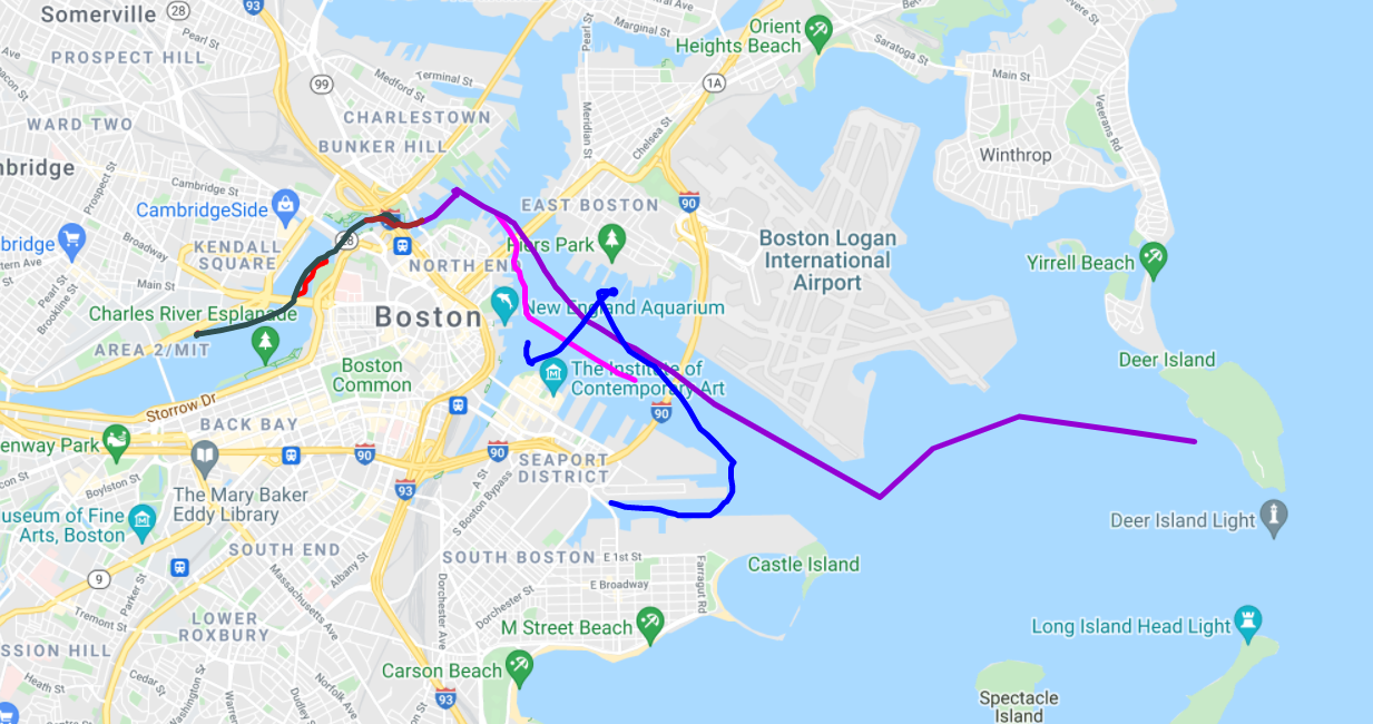
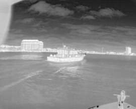
R/V Philos recorded scenes around the Massachusetts Bay area over a period of 2 years from 2019 till November 2021. This gave us an opportunity to create seasonal and temporal diversity in the dataset. Nearshore scenarios were also captured as they present more challenging scenes with construction and increased human and vehicle presence. This was in addition to the complexity present due to weather and light patterns observed in the farther seas. Images were taken in a natural, uncontrolled environment which makes the dataset applicable for practical use. Fig. 4 shows some of the typical routes the ASV has taken in these trips.
R/V Philos stores data from various sensors in the form of rosbag BSD (2020) files. LWIR and optical images were extracted from these rosbag files and carefully analyzed. One challenge faced while selecting LWIR images was the lack of texture and color information that sometimes undermined the scene complexity. In such cases, we used the corresponding optical equivalents to guide through the selection. The epoch time from the rosbag file was also used to specifically target scenes after sunset. This ensured that our dataset specifically included scenes that would pose challenges to the optical sensors. The resolution of 2019 footage was lesser than later recordings and helped create a variation that would be natural in a practical world. The dataset has approximately equal distribution of these images as indicated in Table 2.
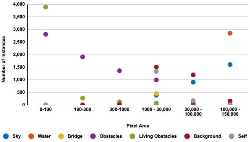
Intrinsically maritime scenes have a significant imbalance in their class distribution as compared to the ground scenes. Sky and water are present in almost any image and occupy major portions. While nearshore scenes help in capturing the real life traffic, and living presence, they also amplify the background adding to the disproportion. As part of the selection process, we tried to reduce this imbalance so that sky and background do not undermine the obstacles and living obstacles in the water that are critical for training. We also focused on bridges as a part of them was relevant for path navigation while the remainder was not and therefore had to be considered as background. Another important difference between maritime and ground scenes is the line of sight. In maritime environment, cameras are exposed to large vistas and distant objects although part of the scene, can only be identified vaguely because they appear tiny. Annotation of such objects may vary as they become more discernible. Such reinterpretation requires consideration of distance as an additional parameter in the classifiers. Table 3 and Fig. 5 show the size and instance distribution of each class in the dataset. The obstacles (purple) and living obstacles (green) mostly occupy less area but there are few instances in which they occupy considerably larger area. The images in such cases contain close up views of boat and/or humans. Fig. 5 shows size variation across far obstacles, sky and water in the order of magnitude.
| Year of recording | Number of images |
|---|---|
| 2019 | 1423 (48.8%) |
| > 2019 | 1493 (51.2%) |
| Total | 2916 |
| Class | Minimum pixel area | Maximum pixel area |
|---|---|---|
| Sky | 303 | 235,763 |
| Water | 3,013 | 251,531 |
| Bridge | 29 | 223,990 |
| Obstacles | 2 | 17,341 |
| Living Obstacles | 2 | 12,512 |
| Background | 48 | 249,720 |
| Self | 32 | 11,915 |
4.2 Image Segmentation
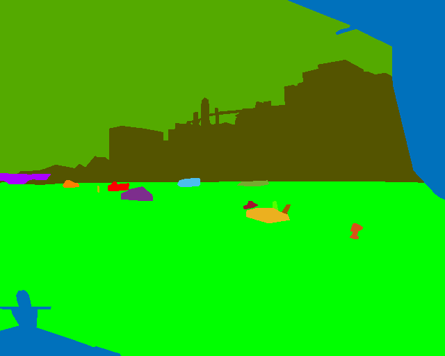
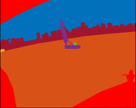
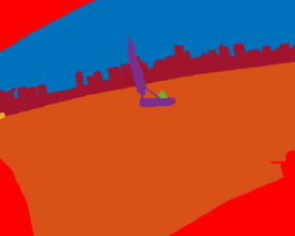
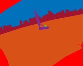
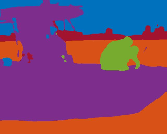
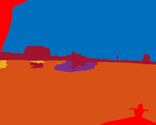
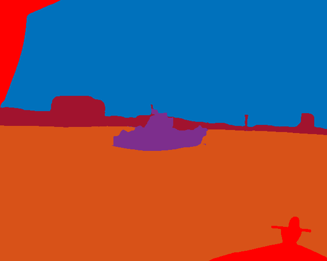
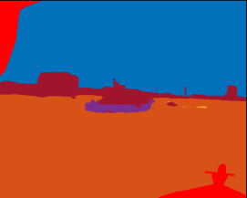
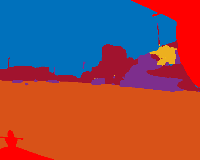
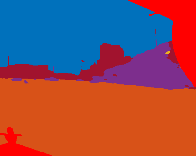
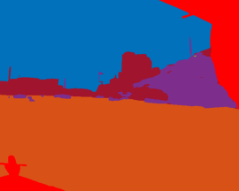
We analyzed the Cityscape Cordts et al. (2016) dataset to understand the guidelines of their classification. In order to make our dataset meaningful for path navigation, we finalized 7 classes - ‘sky’, ‘water’, ‘obstacle’, ‘living obstacle’, ‘bridge’, ‘background’ and ‘self’ for annotation. Categorizing maritime scene into such refined classes ensures that true obstacles are identified and not get combined with other non-essential entities. Segmentation guidelines were prepared to assist the annotators. The ‘obstacle’ class consists of inanimate objects surrounded by water such as buoys, small platforms, sailboats, ships, kayaks. Animate obstacles like humans and birds in the water are classified as ‘living obstacles’. Identification of living entity may be useful for navigation such as deriving COLREGs compliant navigation path IMO (1972) and also for other use cases such as surveillance and environmental or ecological monitoring. Because of the urban setting of the dataset, bridges were frequent and posed a unique challenge. The legs of the bridge that are submerged in water and the belly of the bridge were relevant as the ASV would need to maneuver around the same. However, the top of the bridge or construction on top was not. We decided to annotate the navigation relevant portions of the bridge as ‘bridge’ class and mark the remaining portions as belonging to the ‘background’ class. The ‘background’ class covered any static or dynamic entities that were on land such as trees, buildings, construction cranes and other structures. We observed self returns on the images due to the position of the cameras and these have been labeled as ‘self’ class. This area neither represents ‘obstacle’ nor ‘background’ and hence justified its own label. The path planning module can always be programmed to exclude the ‘self’ class, but it helps to identify the regions in the image correctly. Table 4 shows number of instances in each class that were annotated in these images and also the distribution of pixel area across these classes.
As we were working through the annotations, many images gave us new insights that had to be incorporated. We had anticipated bridge complexity as part of our planning, however we encountered a similar issue with respect to obstacles. Initially we defined an obstacle as an entity surrounded by water on all sides. However, we came across construction objects that stretched from land into the water such as gates that allow the boats to pass through, piers and docks to park the boats, or platforms connected to the land. These obstacles were pertinent for path navigation and hence could not be treated as background. Similarly birds flying just above the water were categorized as sky, and birds in the water were categorized as ‘living obstacle’. Since the images are 2D and LWIR does not give a good feel of the color and texture, there were cases where the obstacle in water was collapsed in the rear background and had to be reviewed thoroughly. Another challenge faced was due to the wide and deep line of sight that we get in the marine environment. There were many obstacles near the horizon that were very tiny. We had to enlarge the image and annotate such images per pixel. A person on a boat is annotated as a ‘living obstacle’ while the boat is annotated as an ‘obstacle’. In cases where the boat was far out and a human could not be easily identified on the boat, it was not called out and considered as part of the ‘obstacle’ class.
| Class | Total number of instances | % Distribution of number of instances | % Distribution of pixel area |
|---|---|---|---|
| Sky | 2902 | 12.97 | 30.58 |
| Water | 2916 | 13.04 | 52.21 |
| Bridge | 715 | 3.19 | 1.67 |
| Obstacles | 7120 | 31.83 | 0.94 |
| Living Obstacles | 4350 | 19.45 | 0.05 |
| Background | 2860 | 12.78 | 11.28 |
| Self | 1501 | 6.71 | 3.25 |
In addition to labeling, we also had to make a choice between semantic and instance segmentation. In semantic segmentation, each occurrence of a class is assigned same class label while in instance segmentation, each instance of a class is assigned different instance id. Unlike on land, maritime environment has a wide and deep line of sight. The near and far objects may overlap in the 2-D view of an image. They will be collapsed if semantic segmentation was used. By instance segmenting the image, the information of overlapping multiple obstacles can be retained which in turn can be used to evaluate or develop occlusion aware classifier vital for path planning. Lastly, the benefit of instance segmentation is that it can always be converted programmatically to semantic based on the need. Fig. 6 illustrates a few samples of raw LWIR images and their annotated masks.

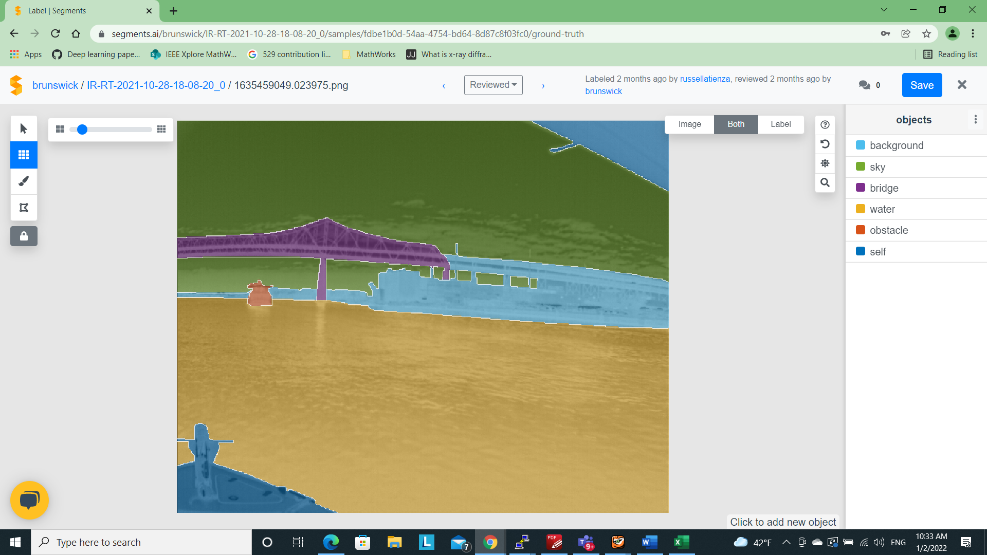
4.3 Labeling Process
An independent organization was tasked with the labeling of these images. To achieve consistency in the result, we created and shared a detailed class label definition document so that labelers would have a common understanding. We also labeled a batch of images ourselves to illustrate the desired outcome. There are many tools available for image segmentation but we chose Debals (2021) platform because of its ease of use. The labeling was quick because of it’s superpixels technology. The API interface made working with the labeled dataset efficient. Fig. 7 shows the tool in action. While the labeling tool was easy to use, there were some challenges faced especially due to the nature of LWIR images. Lack of color and textures posed difficulties in image identification as well as annotation. Color and texture assists the human eye in making a judgment. Lack of thereof, led to multiple reviews in some complex situations such as cluttered set of obstacles, cluster of parking poles, flock of birds or distant ships. For each LWIR video, the corresponding optical version was therefore provided to the labeling team for reference. The image had to be classified in 7 classes. This made the labeling process quite elaborate and time consuming. Identifying parts of the bridge that should be annotated as background was subjective and as a result, there may be some deviations in some of the annotations. In summary, the semantic annotation exercise for LWIR images was more time consuming and needed a lot more attention than we had anticipated.
2 rounds of reviews were done to improve the accuracy of segmentation. Including the reviews, each image annotation took approximately 25 minutes. We also developed a script to check for any unclassified pixels and corrected such masks. Automated checks for validating the segmentation and gathering metrics were also developed.
5 DATASET EVALUATION
Though we have created instance-segmentation dataset, for the purpose of evaluation we used its semantic segmentation masks. To evaluate the efficacy of the dataset, we used 3 image segmentation architectures - UNet developed earlier by Ronneberger et al. (2015) for medical image segmentation, PSPNet by Zhao et al. (2017) for its improvement over fully convolutional network based segmentation and DeepLabv3 by Chen et al. (2018) which is known for its overall superior performance. The dataset was split into 3 categories - 70% for training, 20% for validation and 10% for testing. The test images were used only during inference. Pretrained weights such as Deng et al. (2009) are generally available for training optical images. They greatly reduce the time to retrain the model, however these do not work well for LWIR image training as shown by Nirgudkar and Robinette (2021). We therefore trained these architectures from scratch for our LWIR dataset. Original image resolution of 640512(widthheight) pixels was used across all the architectures - UNet (Ronneberger et al. (2015)), PSPNet (Zhao et al. (2017)), DeepLabv3 (Chen et al. (2018)) for both 2019 as well as the 2020 images.
5.1 Data Augmentation
Robust, diverse and large volume of data is a prerequisite for any successful model. However, creating a labeled dataset is a laborious and expensive task. A common technique employed in increasing the dataset variety is data augmentation Schöller et al. (2019), Bovcon et al. (2019). We used the following 2 types of transformations for our dataset:
-
•
Rotation: An image and its mask were rotated by °, °, °
-
•
Mirror: The original image and mask and their rotated equivalence from previous step was mirrored on the vertical axis
This scheme generated 13 images from 1 image. Accordingly, our dataset was augmented to 40,096 images. An illustrative example is shown in Fig. 8.
5.2 Performance Criterion
Intersection over union (IoU) is an important metric for segmentation inference Csurka et al. (2013). It is defined as ratio of area of intersection between predicted segmentation mask (P) and the ground truth (G), and the area of union between the two.
| (1) |
The IoU score ranges between 0 and 1. A threshold value can be chosen to determine if the inference can be treated as true positive (TP). If the IoU score is greater than a certain threshold then we treat the inference as true positive (TP) otherwise it is treated as false negative (FN). If the ground truth does not contain the region present in prediction then it is treated as false positive (FP). Usually a threshold value of greater than 0.5 is considered optimal Liu et al. (2021), however, if the class sizes are tiny as in the present case, the threshold can be compromised to a lower value. The precision, recall and F1 score are defined as follows:
| (2) |
| (3) |
5.3 Performance Metrics
All 3 architectures were run on Colab (2021) platform which provided a 16GB GPU memory. Training was performed from scratch without using pretrained weights. Images were randomly shuffled prior to the training which helped in improving the robustness of the model. Table 5 gives a summary of the high level metrics obtained for each architecture.
| Test | UNet | PSPNet | DeepLabv3 |


| Name | Images | Image size | Epoch | Loss | Training time |
|---|---|---|---|---|---|
| UNet | train:27678 val:7910 test:4508 | 640*512 | 50 | 0.0202 | 27hr 50min |
| PSPNet | 0.0223 | 47hr 56min | |||
| DeepLabv3 | 0.0112 | 29hr 30min |
| Model | Class | Th | TP | FP | FN | Pr | Re | F1 |
|---|---|---|---|---|---|---|---|---|
| UNet | Sky | 0.6 | 4327 | 24 | 153 | 99.4 | 96.6 | 98.0 |
| DeepLabv3 | 4374 | 8 | 106 | 99.8 | 97.6 | 98.7 | ||
| PSPNet | 4408 | 18 | 72 | 99.6 | 98.4 | 99.0 | ||
| UNet | Water | 0.6 | 4508 | 0 | 0 | 100 | 100 | 100 |
| DeepLabv3 | 4508 | 0 | 0 | 100 | 100 | 100 | ||
| PSPNet | 4508 | 0 | 0 | 100 | 100 | 100 | ||
| UNet | Bridge | 0.6 | 723 | 605 | 409 | 54.4 | 63.9 | 58.8 |
| 0.3 | 962 | 605 | 170 | 61.4 | 85.0 | 71.3 | ||
| DeepLabv3 | 0.6 | 870 | 377 | 262 | 69.8 | 76.9 | 73.1 | |
| 0.3 | 1013 | 377 | 119 | 72.9 | 89.5 | 80.3 | ||
| PSPNet | 0.6 | 910 | 319 | 222 | 74.0 | 80.4 | 77.1 | |
| 0.3 | 1040 | 319 | 92 | 76.5 | 91.9 | 83.5 | ||
| UNet | Obstacle | 0.6 | 615 | 504 | 2193 | 55.0 | 21.9 | 31.3 |
| 0.3 | 1645 | 504 | 1163 | 76.5 | 58.6 | 66.4 | ||
| DeepLabv3 | 0.6 | 1143 | 429 | 1665 | 72.7 | 40.7 | 52.2 | |
| 0.3 | 2045 | 429 | 763 | 82.7 | 72.8 | 77.4 | ||
| PSPNet | 0.6 | 1175 | 428 | 1633 | 73.3 | 41.8 | 53.3 | |
| 0.3 | 2068 | 428 | 740 | 82.9 | 73.6 | 78.0 | ||
| UNet | Living Ob | 0.6 | 98 | 136 | 886 | 41.9 | 10.0 | 16.1 |
| 0.3 | 420 | 136 | 564 | 75.5 | 42.7 | 54.5 | ||
| DeepLabv3 | 0.6 | 294 | 141 | 690 | 67.6 | 29.9 | 41.4 | |
| 0.3 | 599 | 141 | 385 | 80.9 | 60.9 | 69.5 | ||
| PSPNet | 0.6 | 65 | 9 | 1045 | 87.8 | 5.9 | 11.0 | |
| 0.3 | 127 | 9 | 983 | 93.4 | 11.4 | 20.4 | ||
| UNet | Background | 0.6 | 3856 | 85 | 526 | 97.8 | 88.0 | 92.7 |
| DeepLabv3 | 4049 | 33 | 333 | 99.2 | 92.4 | 95.7 | ||
| PSPNet | 4178 | 50 | 204 | 98.8 | 95.3 | 97.0 | ||
| UNet | Self | 0.6 | 2306 | 179 | 74 | 92.8 | 96.9 | 94.8 |
| DeepLabv3 | 2322 | 54 | 58 | 97.7 | 97.6 | 97.6 | ||
| PSPNet | 2329 | 19 | 51 | 99.2 | 97.9 | 98.5 |
The training loss is quite low for all the three architectures. However, since water and sky occupy significant portions of the maritime images, this parameter does not help much and gives misleading accuracy. Classes were therefore individually analyzed and Table 6 reports these metrics at a class level. As noted above, sky and water have a significant contribution in each image and therefore yield a high F1 even with a threshold of 0.6. The classes that are critical for path navigation namely ‘obstacles’, ‘living obstacles’ and ‘bridge’ are much smaller as per Fig. 5. As shown in Table 6, a threshold of 0.6 gives substantial FNs for ‘’obstacles’ and ‘living obstacles’. Since the pixel area of these classes is really tiny, we decided to evaluate their performance by lowering the threshold to 0.3. As seen from the table, the FN reduced appreciably. The threshold value can be subjective based on the size of the class. A value of 0.6 for tiny sizes is too high a bar to achieve. The primary intent of the model is path navigation and having a dynamic threshold based on parameters like size or distance would enable the model to predict the presence of an obstacle although it may have lesser spatial accuracy. Poor recall score of PSPNet on ‘living obstacles’ indicates its failure to identify them which is also reflected in low F1 score.
Fig. 9 indicates the inference results from all 3 architectures for a few sample images. Living obstacles (humans) have been inferred really well in both DeepLabv3 and UNet. The boundaries separating humans from the obstacle (boat) has been interpreted well. In the second row, very tiny obstacles (birds) in the water have been correctly inferred by DeepLabv3 and UNet. Third row indicates that curvature or waves in water pose no issue to the model. Reflection in water in the fourth row, or the heavy cloud cover right on top of the sea, has been interpreted properly by the models. PSPNet was found to have problems with identifying ‘living obstacles’. While it works really well for all other classes, it needs a lot of training to consistently differentiate the boundaries between obstacle and the living obstacle.
In addition to the above limitation in PSPNet, there were some situations where very tiny obstacles were missed or not completely identified. Bridge is another area where the classifiers sometimes gave inconsistent results. This was primarily due to the fact that ground truth for the bridge contained portion annotated as ‘background’ that is not pertinent to navigation. The classifier therefore sometimes incorrectly inferred the navigable portion of the bridge as background and vice versa. Despite that, inference for ‘bridge’ class improved significantly after increasing the training to 50 epochs. Some of the challenge cases are shown in Fig. 10.
| Test | UNet | PSPNet | DeepLabv3 |


To get consistent and meaningful performance from the deep learning models, various modifications were tried and parameters changed. A few of those key modifications are elaborated below:
Initially we had reduced the image size to 320256(widthheight) to speedup the training phase. This resulted in a lot of smaller obstacles being missed in the inference. The obstacles were inherently small as shown in Table 3 and they got tinier with the reduction in image size leaving the classifier with very less information to train well. It was therefore decided to retain the original size of the images. We also experimented with excluding 2019 images because they were of low resolution. We expected improvement in the performance. However,the performance worsened as a lot of variation and information contained in the 2019 dataset was lost. We therefore retained both 2019 and 2020 images.
To increase the dataset size, data augmentation was used as described in Sub-Section 5.1. For optical images, color adjustment is yet another augmentation operation. However, augmentation by changing the brightness of LWIR images had adverse effect on the inference and was not incorporated. Larger rotations (°, °) were tried and that caused distortion in 2019 images and deteriorated the overall results. Smaller range (°, °, °) seem to fit the dataset well. An important consideration that improved the performance drastically was shuffling. Since our images were named based on epoch times, without explicit shuffling they were fed sequentially to the classifier and gave poor results. They were shuffled randomly before the training and that variation helped the classifiers boost the performance multi-fold.
As seen from the inference, horizon detection does not pose a problem in LWIR images. However, there are some sporadic instances of clouds being incorrectly inferred as water and vice versa. This happens mainly when there are white clouds in the sky that appear similar to water, have similar pixel values and get labeled incorrectly. Bridge annotation remained challenging despite good F1 scores. Depending on the nature of the bridge and position of the background with respect to the bridge, the classifier has a challenge and classifies the navigable portion of the bridge as a background. When the bridge has arches, view from beneath the arch could be sky or background and water. Such minute details pleasantly have been represented well most of the times, but do pose a challenge in other cases.
In summary, standard CNN architectures can be trained with LWIR images and can produce good inference. The LWIR dataset indeed complements the optical dataset in many such scenarios and is therefore invaluable in the perception task.
6 CONCLUSION
We have presented a comprehensive MassMIND dataset containing over 2,900 segmented diverse LWIR images and made it publicly available. This is the first maritime dataset that segments LWIR images in 7 different classes with emphasis on living and non-living, static and dynamic obstacles in the water. The dataset is also evaluated and bench marked against a few industry standard architectures.
Of the 3 classifiers evaluated, DeepLabv3 Chen et al. (2018) stands out the best, followed by UNet and PSPNet. PSPNet is found to be comparable to DeepLabv3 in all other classes except for living obstacles. Our research calls out significance of LWIR when it comes to problems such as extreme light conditions and horizon detection that are common in the optical world. In addition, the dataset tries to encompass many of the critical aspects of the maritime imagery such as static and dynamic obstacles of varying sizes, crowded shoreline, deep seas, varying weather and light patterns, and life presence on the water surface. Such a diverse LWIR dataset can be useful to improve the deep learning architectures for the maritime environment. At the same time, it can complement optical datasets. The present dataset also has some limitations. Certain obstacles such as river barges or Sea-Doos are not captured because of the ASVs’ urban setting. The demographics within the dataset is also limited to one region in USA. We understand that as a result, there is no variety in navigational markers used across world regions. This gap can be bridged by collaboration with other researchers.
We plan to refine the current ’obstacle’ class to indicate the type of obstacle such as sailboats, kayaks, and merchant ships. This will enable creation of COLREG compliant classifiers. We plan to integrate the inference obtained from these models in real time with the perception pipeline developed by Clunie et al. (2021). Lastly, we will also explore creation of an instance-segmentation architecture dedicated towards LWIR images in the marine environment.
We are grateful to Brunswick® Corporation for their support. The views, opinions and/or findings expressed are those of the authors and should not be interpreted as representing the official views of Brunswick® Corporation. We also thank the team at segments.ai for providing early access free of charge and for providing dashboard for tracking the progress of the labeling work.
The Authors declare that there is no conflict of interest.
References
- AUVLab (1989) AUVLab (1989) MIT Sea Grant, Autonomous Underwater Vehicles Lab URL https://seagrant.mit.edu/auv-lab/.
- Bloisi et al. (2015) Bloisi D, Iocchi L, Pennisi A and Tombolini L (2015) ARGOS-Venice Boat Classification. 12th IEEE International Conference on Advanced Video and Signal Based Surveillance (AVSS) : 1–610.1109/AVSS.2015.7301727.
- Bovcon and Kristan (2020) Bovcon B and Kristan M (2020) A water-obstacle separation and refinement network for unmanned surface vehicles. 2020 IEEE International Conference on Robotics and Automation, ICRA 2020, Paris, France, May 31 - August 31, 2020 : 9470–947610.1109/ICRA40945.2020.9197194. URL https://doi.org/10.1109/ICRA40945.2020.9197194.
- Bovcon et al. (2019) Bovcon B, Muhovič J, Perš J and Kristan M (2019) The MaSTr1325 dataset for training deep usv obstacle detection models. IEEE/RSJ International Conference on Intelligent Robots and Systems (IROS) .
- Bovcon et al. (2021) Bovcon B, Muhovič J, Vranac D, Mozetič D, Perš J and Kristan M (2021) MODS- A USV-oriented object detection and obstacle segmentation benchmark .
- BSD (2020) BSD (2020) Rosbag package URL http://wiki.ros.org/rosbag.
- Castellini et al. (2020) Castellini A, Bloisi D, Blum J, Masillo F and Farinelli A (2020) Intcatch Aquatic Drone Sensor Dataset. Mendeley Data, V2 10.17632/gtt7stf5x8.2.
- Chen et al. (2018) Chen L, Papandreou G, Kokkinos I, Murphy K and Yuille A (2018) Deeplab: Semantic image segmentation with deep convolutional nets, atrous convolution, and fully connected CRFs. IEEE TPAMI 40(4): 834–848.
- Clunie et al. (2021) Clunie T, DeFilippo M, Sacarny M and Robinette P (2021) Development of a perception system for an autonomous surface vehicle using monocular camera, lidar, and marine radar. International Conference on Robotics and Automation .
- Colab (2021) Colab (2021) Making the most of your Colab URL https://colab.research.google.com/.
- Cordts et al. (2016) Cordts M, Omran M, Ramos S, Rehfeld T, Enzweiler M, Benenson R, Franke U, Roth S and Schiele B (2016) The Cityscapes Dataset for Semantic Urban Scene Understanding. Proc. of the IEEE Conference on Computer Vision and Pattern Recognition (CVPR) .
- Csurka et al. (2013) Csurka G, Larlus D, Perronnin F and Meylan F (2013) What is a good evaluation measure for semantic segmentation?. Bmvc 27(2013): 10–5244.
- Debals (2021) Debals O (2021) Platform for Image Segmentation URL https://segments.ai.
- DeFilippo et al. (2021) DeFilippo M, Sacarny M and Robinette P (2021) RoboWhaler: A Robotic Vessel for Marine Autonomy and Dataset Collection. OCEANS .
- Deng et al. (2009) Deng J, Dong W, Socher R, Li LJ, Li K and Fei-Fei L (2009) Imagenet: A large scale hierarchical database. CVPR : 248–255.
- EO (2022) EO (2022) What is SWIR? URL https://www.edmundoptics.com/knowledge-center/application-notes/imaging/what-is-swir/?utm_medium=email&utm_source=transaction.
- Hyll (2016) Hyll K (2016) Image-based quantitative infrared analysis and microparticle characterisation for pulp and paper applications 10.13140/RG.2.1.2595.6884.
- IMO (1972) IMO (1972) COLREGs: Convention on the International Regulations for Preventing Collisions at Sea .
- Krizhevsky et al. (2012) Krizhevsky A, Sutskever I and Hinton G (2012) Imagenet classification with deep convolutional neural networks. Advances in Neural Information Processing Systems 25: 1097–1105.
- Liu et al. (2021) Liu J, Geng Y, Zhao J, Zhang K and Li W (2021) Image Semantic Segmentation Use Multiple-threshold Probabilistic R-CNN with Feature Fusion. Symmetry .
- NASA (2003) NASA (2003) Near, Mid and Far Infrared URL http://www.icc.dur.ac.uk/~tt/Lectures/Galaxies/Images/Infrared/Regions/irregions.html.
- Nirgudkar et al. (2022) Nirgudkar S, DeFilippo M, Sacarny M, Benjamin M and Robinette P (2022) MassMIND: Massachusetts Maritime INfrared Dataset URL https://github.com/uml-marine-robotics/MassMIND.
- Nirgudkar and Robinette (2021) Nirgudkar S and Robinette P (2021) Beyond visible light: Object Detection Using Long Wave Infrared Images in Maritime Environment. International Conference on Autonomous Robotics .
- Patino et al. (2016) Patino L, Cane T, Vallee A and Ferryman J (2016) PETS 2016: Dataset and Challenge. IEEE Conference on Computer Vision and Pattern Recognition Workshops (CVPRW) : 1240–124710.1109/CVPRW.2016.157.
- Prasad et al. (2017) Prasad DK, Rajan D, Rachmawati L, Rajabaly E and Quek C (2017) Video Processing from Electro-optical Sensors for Object Detection and Tracking in Maritime Environment: A Survey. IEEE Transactions on Intelligent Transportation Systems 18(8): 1993–2016.
- Qi et al. (2011) Qi B, Wu T, Dai B and He H (2011) Fast detection of small infrared objects in maritime scenes using local minimum patterns. 18th IEEE International Conference on Image Processing : 3553–355610.1109/ICIP.2011.6116483.
- Ribeiro (2015) Ribeiro R (2015) The Sea-gull Dataset URL http://vislab.isr.ist.utl.pt/seagull-dataset.
- Robinette et al. (2019) Robinette P, Sacarny M, DeFilippo M, Novitzky M and Benjamin MR (2019) Sensor evaluation for autonomous surface vehicles in inland waterways. OCEANS .
- Rodin and Johansen (2018) Rodin CD and Johansen TA (2018) Detectability of Objects at the Sea Surface in Visible Light and Thermal Camera Images. OCEANS - MTS/IEEE Kobe Techno-Oceans (OTO) 10.1109/OCEANSKOBE.2018.8559310.
- Ronneberger et al. (2015) Ronneberger O, Fischer P and Brox T (2015) U-Net: Convolutional Networks for Biomedical Image Segmentation. Medical Image Computing and Computer-Assisted Intervention (MICCAI) 9351: 234–241. 10.1007/978-3-319-24574-4_28.
- Schöller et al. (2019) Schöller FET, Plenge-Feidenhans’l MK, Stets JD and Blanke M (2019) Assessing Deep-learning Methods for Object Detection at Sea from LWIR Images. International federation of automatic control workshop 52(21): 64–71. 10.1109/OCEANSKOBE.2018.8559310.
- SeaGrant (2022) SeaGrant (2022) MIT Sea Grant Marine Perception Dataset URL https://seagrant.mit.edu/auvlab-datasets-marine-perception-1.
- Steccanella et al. (2020) Steccanella L, Bloisi D, Castellini A and Farinelli A (2020) Waterline and Obstacle Detection in Images from Low-Cost Autonomous Boats for Environmental Monitoring. Robotics and Autonomous Systems 10.1016/j.robot.2019.103346.
- Wang et al. (2017) Wang B, Dong L, Zhao M and Xu W (2017) Fast infrared maritime target detection: Binarization via histogram curve transformation. Infrared Physics and Technology 83: 32–44. 10.1016/j.infrared.2017.03.009.
- Zhang et al. (2015) Zhang MM, Choi J, Daniilidis K, Wolf MT and Kanan C (2015) VAIS: A dataset for recognizing maritime imagery in the visible and infrared spectrums. IEEE Conference on Computer Vision and Pattern Recognition Workshops (CVPRW) : 10–1610.1109/CVPRW.2015.7301291.
- Zhao et al. (2017) Zhao H, Shi J, Qi X, Wang X and Jia J (2017) Pyramid Scene Parsing Network. IEEE Conference on Computer Vision and Pattern Recognition (CVPR) : 6230–623910.1109/CVPR.2017.660.